Download to read offline
![2
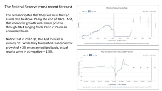
Are we already in a recession? Maybe …
2022 Q1 GDP growth was already negative. And, 2022 Q2 may very well be [negative] when the released
data comes out.
The majority of the financial media believes we are already in a recession because of the stubbornly high
inflation (due to supply chain bottlenecks) and the Federal Reserve aggressive monetary policy to fight
inflation. The policy includes a rapid rise in short-term rates, and a reversing of the Quantitative Easing bond
purchase program (reducing the Fed’s balance sheet and taking liquidity & credit out of the financial system).
The Bearish stock market also suggests we are currently in a recession.
On the other hand, Government authorities including the President, the Secretary of the Treasury (Janet
Yellen), and the Federal Reserve all believe that the US economy can achieve a “soft landing” with a declining
inflation rate, while maintaining positive economic growth.
I developed a couple of models to attempt to predict recessions using historical data.](https://image.slidesharecdn.com/recessions-220621184255-f2c5bbf8/85/Recessions-pptx-2-320.jpg)
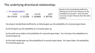

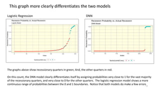
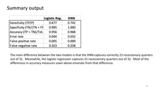
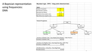
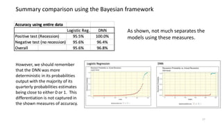
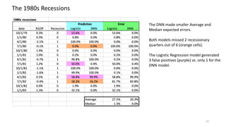
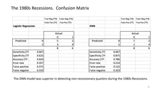
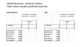
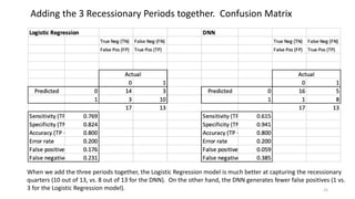
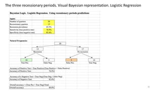
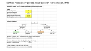
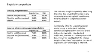

The document discusses predicting recessions using logistic regression and deep neural networks (DNNs), highlighting that the U.S. economy may already be in a recession with negative GDP growth and high inflation influences. Two models were developed to predict recessions, with the DNN showing slightly superior performance in some historical recession periods, though neither model successfully predicted the potential recession beginning in Q1 2022. Ultimately, the models demonstrate varying accuracies and limitations, particularly in forecasting future recessions accurately due to the difficulty in predicting key independent variables.