Download to read offline


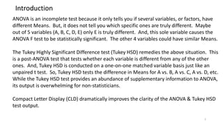
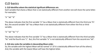
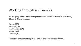
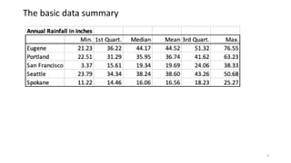
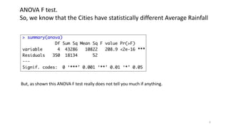
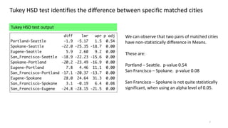
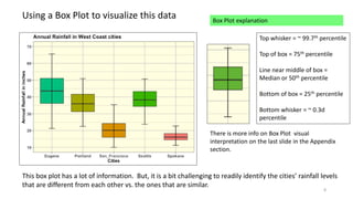
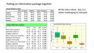
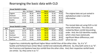
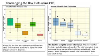
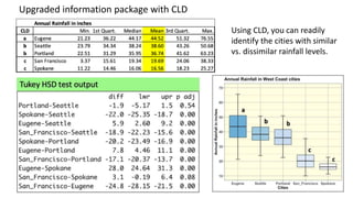

The document explains the limitations of ANOVA in identifying specific differences between variables and introduces the Tukey HSD test as a solution. It highlights the Compact Letter Display (CLD) method, which enhances the clarity of test outputs by visually representing significant differences and ranking variables. An example using rainfall data from five West Coast cities demonstrates how CLD can effectively convey statistical results and comparisons.