Comparison of Time Domain Techniques for the Evaluation of the Response and the Stability in Long Span Suspension Bridges
•
1 like•577 views

During the last decades, several studies on suspension bridges under wind actions have been developed in civil engineering and many techniques have been used to approach this structural problem both in time and frequency domain. In this paper, four types of time domain techniques to evaluate the response and the stability of a long span suspension bridge are implemented: nonaeroelastic, steady, quasi steady, modified quasi steady. These techniques are compared considering both nonturbulent and turbulent flow wind modelling. The results show consistent differences both in the amplitude of the response and in the value of critical wind velocity.
![F. Petrini et al. / Computers and Structures 85 (2007) 1032–1048
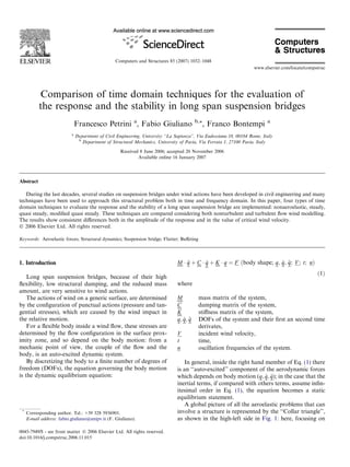
aeroelastic forces dependences, aeroelastic problems are
classified in three categories:
1. Response problems, in which there is a dynamic equilibrium between the body and the wind forces: the expression of the forces contain time-independent terms.
2. Stability problems, in which the interchanging energy
between the body motion and the aeroelastic forces, produces a gradual and unlimited increment of the motion
energy, leading to the dynamic equilibrium instability at
‘‘critical velocities’’. For these problems, the expression
of the forces does not contain time-independent terms.
3. Mixed (stability and response) problems, in which incident wind velocities are close to the critical velocities
and the expression of the forces contains both time-independent and auto-excited terms.
In instability problems, the forces are usually transferred
in the left side hand of the equation in order to obtain a
homogeneous equation in which mass, damping, and stiffness matrices contain auto-excited coefficients.
Considering a generic structure under wind action, two
principal approaches exist to solve the relative aeroelastic
problem:
1. Frequency domain approach, usual for instability problems, based on a modal combinations for the structural
system, is less reliable for structures with strong nonlinear nature.
1033
2. Time domain approach, requiring a time integration of
the equations of the motions of the structure subjected
to wind loads, with large computational costs for structure with many DOFs.
In the present paper, the time domain approach has
been adopted to study the response and the stability problem of a long span suspension bridge under wind actions.
In particular, the incident wind has been modelled as a turbulent flow for the response problem, while for the stability
problem, it has been modelled as nonturbulent.
2. Aeroelastic forces for suspension bridges
In the last decades, referring to aeronautic engineering,
civil engineers have developed many analytical theories to
model wind effects on structures, and simplified approaches
have been adopted to evaluate the aeroelastic terms,
because of the very complex dependence above listed. Both
frequency and time domain techniques to model aeroelastic
forces, derive from wing theory [1–3,5].
In the case of suspension bridges, two peculiar aspects
have to be considered. First, suspension bridges deck sections, usually have so-called ‘‘semi-bluff’’ or ‘‘bluff’’ body
shapes, with (opposite to wing shapes) well predictable
points of flow detachments along the deck surfaces (‘‘live
edges’’), where the turbulence of the flow is very high.
The second particular aspect is related to the intrinsic
turbulent content of an incident wind flow. Furthermore
Collar
Static aeroelastic
stability
Forces: A=Aeroelastic; E=Elastic; I=Inertial; F=Applied
Equilibrium equation:
D
Galloping
G
Vortex Shedding
VS
Flutter
F
Buffeting
B
A− E = 0
For
stability
A+E+I+F=0
Torsional divergence
Dynamic aeroelastic
stability
A+ I − E = 0
Aeroelastic
problems
Static aeroelastic
response
A+ F −E = 0
For
Response
Aeroelastic Phenomena
Tors. Divergence
V. Shedding
Galloping
Classical flutter
Stall flutter
Buffeting
Non Aeroelastic Sciences
D
VS
G
Fc
Fs
B
Mechanics of
vibrations
Mechanics of
rigid body flight
Dynamic aeroelastic
response
MV
MR
A+ I − E + F = 0
Torsional divergence
Galloping
Vortex Shedding
Flutter
Buffeting
Static instability in which
torsional moment due to
aeroelastic forces, overcomes
the elastic resistant moment of
the body
An asymmetry in the flow
produces a vertical oscillation
that generate oscillations in
aerodynamic forces, which
depends on body oscillations
velocity and involves an
aerodynamic damping, which is
opposite to the structural
damping.
If
aerodynamic
damping is greater than the
structural one, the motion may
become unstable.
Dynamic instability very similar
to a resonance. Some vortex
loose themselves in the wake
behind the body. Such physic
configuration generates an
oscillation in aerodynamic
forces,
with
a
definite
frequency. In a certain range of
wind velocity, the oscillation
frequency of the forces “block”
the
structural
oscillations
frequency and it governs the
structural oscillation period.
Dynamic instability in which
two d.o.f. of the forced
structural system are coupled
and,
under
opportune
configurations (defined “critic”)
for frequencies and reciprocal
phase angles, lead the damping
of the system to become
negative, and the oscillations
increase in amplitude
Motion under the action of time
random variable forces both in
intensity and direction. The
buffeting phenomenon assumes
aeroelastic
importance
in
concomitance
of
other
aeroelastic phenomena (like
Flutter or Vortex shedding).
Fig. 1. Aeroelastic problems and instabilities.
A classic buffeting effect, is the
one generated by the intrinsic
turbulence
within
the
atmospheric boundary layer.](data:image/gif;base64,R0lGODlhAQABAIAAAAAAAP///yH5BAEAAAAALAAAAAABAAEAAAIBRAA7)
Recommended
Recommended
More Related Content
What's hot
What's hot (17)
Similar to Comparison of Time Domain Techniques for the Evaluation of the Response and the Stability in Long Span Suspension Bridges
Similar to Comparison of Time Domain Techniques for the Evaluation of the Response and the Stability in Long Span Suspension Bridges (20)
More from Franco Bontempi Org Didattica
More from Franco Bontempi Org Didattica (20)
Recently uploaded
Recently uploaded (20)
Comparison of Time Domain Techniques for the Evaluation of the Response and the Stability in Long Span Suspension Bridges
- 1. Computers and Structures 85 (2007) 1032–1048 www.elsevier.com/locate/compstruc Comparison of time domain techniques for the evaluation of the response and the stability in long span suspension bridges Francesco Petrini a, Fabio Giuliano a b,* , Franco Bontempi a Department of Civil Engineering, University ‘‘La Sapienza’’, Via Eudossiana 18, 00184 Rome, Italy b Department of Structural Mechanics, University of Pavia, Via Ferrata 1, 27100 Pavia, Italy Received 8 June 2006; accepted 20 November 2006 Available online 16 January 2007 Abstract During the last decades, several studies on suspension bridges under wind actions have been developed in civil engineering and many techniques have been used to approach this structural problem both in time and frequency domain. In this paper, four types of time domain techniques to evaluate the response and the stability of a long span suspension bridge are implemented: nonaeroelastic, steady, quasi steady, modified quasi steady. These techniques are compared considering both nonturbulent and turbulent flow wind modelling. The results show consistent differences both in the amplitude of the response and in the value of critical wind velocity. Ó 2006 Elsevier Ltd. All rights reserved. Keywords: Aeroelastic forces; Structural dynamics; Suspension bridge; Flutter; Buffeting 1. Introduction Long span suspension bridges, because of their high flexibility, low structural damping, and the reduced mass amount, are very sensitive to wind actions. The actions of wind on a generic surface, are determined by the configuration of punctual actions (pressure and tangential stresses), which are caused by the wind impact in the relative motion. For a flexible body inside a wind flow, these stresses are determined by the flow configuration in the surface proximity zone, and so depend on the body motion: from a mechanic point of view, the couple of the flow and the body, is an auto-excited dynamic system. By discretizing the body to a finite number of degrees of freedom (DOFs), the equation governing the body motion is the dynamic equilibrium equation: * Corresponding author. Tel.: +39 328 5936901. E-mail address: fabio.giuliano@unipv.it (F. Giuliano). 0045-7949/$ - see front matter Ó 2006 Elsevier Ltd. All rights reserved. doi:10.1016/j.compstruc.2006.11.015 _ _ q M Á € þ C Á q þ K Á q ¼ F ðbody shape; q; q; €; V ; t; nÞ q ð1Þ where M C K _ q q; q; € V t n mass matrix of the system, damping matrix of the system, stiffness matrix of the system, DOFs of the system and their first an second time derivates, incident wind velocity, time, oscillation frequencies of the system. In general, inside the right hand member of Eq. (1) there is an ‘‘auto-excited’’ component of the aerodynamic forces _ q which depends on body motion (q; q; €); in the case that the inertial terms, if compared with others terms, assume infinitesimal order in Eq. (1), the equation becomes a static equilibrium statement. A global picture of all the aeroelastic problems that can involve a structure is represented by the ‘‘Collar triangle’’, as shown in the high-left side in Fig. 1: here, focusing on
- 2. F. Petrini et al. / Computers and Structures 85 (2007) 1032–1048 aeroelastic forces dependences, aeroelastic problems are classified in three categories: 1. Response problems, in which there is a dynamic equilibrium between the body and the wind forces: the expression of the forces contain time-independent terms. 2. Stability problems, in which the interchanging energy between the body motion and the aeroelastic forces, produces a gradual and unlimited increment of the motion energy, leading to the dynamic equilibrium instability at ‘‘critical velocities’’. For these problems, the expression of the forces does not contain time-independent terms. 3. Mixed (stability and response) problems, in which incident wind velocities are close to the critical velocities and the expression of the forces contains both time-independent and auto-excited terms. In instability problems, the forces are usually transferred in the left side hand of the equation in order to obtain a homogeneous equation in which mass, damping, and stiffness matrices contain auto-excited coefficients. Considering a generic structure under wind action, two principal approaches exist to solve the relative aeroelastic problem: 1. Frequency domain approach, usual for instability problems, based on a modal combinations for the structural system, is less reliable for structures with strong nonlinear nature. 1033 2. Time domain approach, requiring a time integration of the equations of the motions of the structure subjected to wind loads, with large computational costs for structure with many DOFs. In the present paper, the time domain approach has been adopted to study the response and the stability problem of a long span suspension bridge under wind actions. In particular, the incident wind has been modelled as a turbulent flow for the response problem, while for the stability problem, it has been modelled as nonturbulent. 2. Aeroelastic forces for suspension bridges In the last decades, referring to aeronautic engineering, civil engineers have developed many analytical theories to model wind effects on structures, and simplified approaches have been adopted to evaluate the aeroelastic terms, because of the very complex dependence above listed. Both frequency and time domain techniques to model aeroelastic forces, derive from wing theory [1–3,5]. In the case of suspension bridges, two peculiar aspects have to be considered. First, suspension bridges deck sections, usually have so-called ‘‘semi-bluff’’ or ‘‘bluff’’ body shapes, with (opposite to wing shapes) well predictable points of flow detachments along the deck surfaces (‘‘live edges’’), where the turbulence of the flow is very high. The second particular aspect is related to the intrinsic turbulent content of an incident wind flow. Furthermore Collar Static aeroelastic stability Forces: A=Aeroelastic; E=Elastic; I=Inertial; F=Applied Equilibrium equation: D Galloping G Vortex Shedding VS Flutter F Buffeting B A− E = 0 For stability A+E+I+F=0 Torsional divergence Dynamic aeroelastic stability A+ I − E = 0 Aeroelastic problems Static aeroelastic response A+ F −E = 0 For Response Aeroelastic Phenomena Tors. Divergence V. Shedding Galloping Classical flutter Stall flutter Buffeting Non Aeroelastic Sciences D VS G Fc Fs B Mechanics of vibrations Mechanics of rigid body flight Dynamic aeroelastic response MV MR A+ I − E + F = 0 Torsional divergence Galloping Vortex Shedding Flutter Buffeting Static instability in which torsional moment due to aeroelastic forces, overcomes the elastic resistant moment of the body An asymmetry in the flow produces a vertical oscillation that generate oscillations in aerodynamic forces, which depends on body oscillations velocity and involves an aerodynamic damping, which is opposite to the structural damping. If aerodynamic damping is greater than the structural one, the motion may become unstable. Dynamic instability very similar to a resonance. Some vortex loose themselves in the wake behind the body. Such physic configuration generates an oscillation in aerodynamic forces, with a definite frequency. In a certain range of wind velocity, the oscillation frequency of the forces “block” the structural oscillations frequency and it governs the structural oscillation period. Dynamic instability in which two d.o.f. of the forced structural system are coupled and, under opportune configurations (defined “critic”) for frequencies and reciprocal phase angles, lead the damping of the system to become negative, and the oscillations increase in amplitude Motion under the action of time random variable forces both in intensity and direction. The buffeting phenomenon assumes aeroelastic importance in concomitance of other aeroelastic phenomena (like Flutter or Vortex shedding). Fig. 1. Aeroelastic problems and instabilities. A classic buffeting effect, is the one generated by the intrinsic turbulence within the atmospheric boundary layer.
- 3. 1034 F. Petrini et al. / Computers and Structures 85 (2007) 1032–1048 a larger complexity and rotationally nature of the flow determines a larger ‘‘aerodynamic delay’’, which is the transient effect due to the adjustment time of aerodynamic field, in consequence of a changing in body geometric configuration (i.e. rotation and displacements of the deck). In order to take into account these effects, the so-called ‘‘memory terms’’, which consider the influence of displacements history in the expression of the aeroelastic forces, are introduced. These terms are usual implemented by integral expressions [6]. The uncertainties related to the above phenomena lead to the use of the experimental approach. In this sense, studies conduced by Scanlan and Tomko [7], Jain et al. [8] and Scanlan and Simiu [9] had great relevance in wind engineering. Following Scanlan theory, the Self-Excited (SE) components of the aeroelastic forces are determined by a superposition of the effects, referring to the forces obtained by wind tunnel tests, acting on a sectional model of the deck that is moving in simple harmonic oscillations along three sectional DOFs (the rotational and the two translational ones). Referring to Fig. 2, it results for the Lift force _ _ _ LSE ðp; p; h; h; #; #; k; xÞ " _ _ 1 BÁ# h 2 ¼ Á q Á V Á B Á k Á H Ã ðkÞ Á þ k Á H Ã ðkÞ Á 1 2 2 V V _ h p þ k 2 Á H Ã ðkÞ Á # þ k 2 Á H Ã Á þ k Á H Ã ðkÞ Á 3 4 5 B V # p 2 Ã þ k Á H 6 ðkÞ Á B ð2Þ where Analogous expressions of (2) can be written for drag force and moment. 3. Aeroelastic forces in time domain Time domain approaches allow to consider directly the structural nonlinear effects and this is relevant for certain types of structures, like long span suspension bridges. Furthermore, because the time domain analyses outputs are merely the time histories of specific variables, it is the most convenient approach in response problems. Unfortunately, expressions in time domain which consider aspects previously mentioned are not trivial to implement. Consequently in the last years simplified formulations for aeroelastic forces have been developed and improved. The analysis in the time domain consists in a time integration that involves the time step updating of kinematic parameters and acting forces. Referring to Fig. 3, where the problem is represented like a two-dimensional problem, horizontal and vertical components of absolute wind turbulent velocity V a ðtÞ, are considered as composed by mean components U, W, and fluctuant (or turbulent) components uðtÞ and wðtÞ. The resulting absolute velocity is not horizontal, and has a time-varying instantaneous angle of incidence. Adopting the general notation previously introduced (Eq. (1)), one has, for the system DOFs, qT ¼ ½ s h # Š. Moreover, the dependence of the forces from structural DOFs and their time derivatives can be generally expressed in matrix form as: _ q _ F ðq; q; €; nÞ ¼ P ðt; nÞ Á € þ Qðt; nÞ Á q þ Rðt; nÞ Á q q k ¼ xÁB reduced frequency of the system, in simple harV monic motion, H Ã ðkÞ functions of the reduced frequency, i B characteristic dimension of the bridge deck, x circular frequency of the system, in simple harmonic motion, V incident wind velocity. The functions H Ã ðkÞ are called ‘‘flutter derivatives’’ of i the bridge deck, and are determined by wind tunnel tests, imposing simple harmonic motion to the deck model. where the time dependence of DOFs has not been noticed: P ðt; nÞ; Qðt; nÞ and Rðt; nÞ represent in expression (3) coefficient matrices which, in the most general case, depends on time and on oscillation frequency of the system. Principal characteristics of the various aeroelastic theories, are summarized in Table 1: it is clear the overall complexity of the classification, while the most used time domain techniques are presented below. L(t2) L(t1) M(t1) M(t2) D(t2) D(t1) ϑ B y V p x L(t2) ϑ ð3Þ α h M(t2) D(t2) Va(t2) y L(t1) x h M(t1) D(t1) Vy=W+w Vx=U+u B p Fig. 2. Bridge deck section under wind action. Fig. 3. Bridge deck section under turbulent wind action.
- 4. F. Petrini et al. / Computers and Structures 85 (2007) 1032–1048 1035 Table 1 Aeroelastic theories Level Theory Hypothesis and approximations _ q General form F ðq; q; €; t; nÞ (Ref. [9]) S.E.P.a Aerodynamic coefficients X DOFs dependences X X X X Static Static Static Dynamic X X X Dynamic X X X Dynamic Dependent from n Nonlinearised polar lines qðtÞ qðtÞ €ðtÞ _ q 0 1 2 3 Nonaeroelastic (NO) Steady (ST) Quasi Steady (QS) Modified Quasi Steady (QSM) Extension of Aeroelastic Derivates in Time Domain (ADTD) Scanlan Theory (NSS) 4 4 a R R Á qðtÞ R Á qðtÞ þ QÁqðtÞ _ _ RðtÞ Á qðtÞ þ QðtÞ Á qðtÞ X X X X X _ q P ðt; nÞ Á € þ Qðt; nÞ Á q þ Rðt; nÞ Á q X X Frequency domain X X X S.E.P. = Superposition of Effects Principle (concerning the determination of the actions). 3.1. Nonaeroelastic theory (NO) This is a ‘‘zero level’’ aeroelastic theory: aeroelastic effects are not considered in the forces formulation but only the relative angle of incidence between wind and deck, change with time just in accordance with the turbulence of the incident wind. Adopting the small displacements hypothesis, (linearised lift and moment polar line), it results 1 2 DðtÞ ¼ q Á jV a ðtÞj Á B Á cD ½aðtÞŠ 2 1 2 LðtÞ ¼ q Á jV a ðtÞj Á B Á K L0 Á aðtÞ 2 1 2 MðtÞ ¼ q Á jV a ðtÞj Á B2 Á K M0 Á aðtÞ 2 ð4Þ where a is the angle of attack, cD is drag coefficient and KL0, KM0 are the angular coefficients of lift and moment polar diagrams, respectively. 1 2 DðtÞ ¼ q Á jV a ðtÞj Á B Á cD ½cðtÞŠ 2 1 2 LðtÞ ¼ q Á jV a ðtÞj Á B Á cL ½cðtÞŠ 2 1 2 MðtÞ ¼ q Á jV a ðtÞj Á B2 Á cM ½cðtÞŠ 2 ð6Þ Adopting the general formulation of Eq. (3), one can write F ¼ F ðq; tÞ ¼ R Á qðtÞ ð7Þ The steady theory has the appeal of simplicity; furthermore, in the case of nonturbulent incident wind, it shows the fundamental mechanisms of a flutter stability problem (coalescence of frequency, influence of structural parameters, etc.). Nevertheless it implies many approximations, such as the neglecting of the dependence of aeroelastic forces on structural velocities, accelerations and oscillation frequency, and the linearisation of the relation between aeroelastic forces and structural DOFs. Furthermore, the steady theory does not consider the aerodynamic delay, and utilizes static aerodynamic coefficients. 3.2. Steady theory (ST) 3.3. Quasi Steady theory (QS) This is a ‘‘first level’’ aeroelastic theory, where the relative angle of incidence between wind and deck, changes with time due to both the incident wind turbulence and the rotation (torsion) of the deck. Supposing that the bridge deck section rotates around a mean equilibrium position # ¼ #0 , adopting the small displacements hypothesis (both lift and moment polar diagrams are linearised), the aerodynamic coefficients become It is a ‘‘second level’’ aeroelastic theory: instantaneous aeroelastic forces acting on the structure are the same that act on the structure itself when it moves with constant translational and rotational velocities, equal to the real instantaneous ones. The main assumption consists in considering that the body (deck section) is motionless, together with the wind having velocities and directions equal to the instantaneous relative (wind-deck) ones: such assumption is represented in Fig. 4. _ The coefficients of # (bi, with i ¼ L; M) should be derived experimentally by wind tunnel tests [10]; it can be derived also through the use of Computational Fluid Dynamic (CFD) techniques [11,12]. Adopting the hypothesis of small displacements around the mean configuration, Eq. (5) are also valid and the cL ðcÞ ¼ cL ð#0 Þ þ K L0 Á ðc À #0 Þ cM ðcÞ ¼ cM ð#0 Þ þ K M0 Á ðc À #0 Þ ð5Þ in which KL0 and KM0 are the angular coefficients of polar lines computed in # ¼ #0 . Referring to Fig. 3 and defining cðtÞ ¼ aðtÞ À #ðtÞ, the aeroelastic forces are expressed as
- 5. 1036 F. Petrini et al. / Computers and Structures 85 (2007) 1032–1048 1 DðtÞ ¼ q Á jV aL ðtÞj2 Á B Á cD ½cðtÞŠ 2 1 2 LðtÞ ¼ q Á jV aL ðtÞj Á B Á cà ½cðtÞŠ L 2 L(t2) M(t2) D(t2) · · h h − h + bi ⋅ B ⋅ ϑ Va(t2) y ϑ β α x L(t1) h 1 2 MðtÞ ¼ q Á jV aM ðtÞj Á B2 Á cà ½cðtÞŠ M 2 M(t1) D(t1) Vy=W+w ð10Þ · h Vx=U+u − p 2 where ci ðtÞ, jV ai ðtÞj (i ¼ L; MÞ and cD, have the same meaning as the previous expressions included in QS theory. In the expressions (10), aerodynamic coefficients cà and cà L M are dynamic and they are computed like below B p Fig. 4. Quasi steady theory assumption. expressions of aeroelastic forces are identical (in the form) _ _ V ðtÞÀhþbi ÁBÁ#ðtÞ to the steady theory ones, with bi ðtÞ ¼ arctg y V x Àp _ (i ¼ L; M) in substitution of aðtÞ: 1 2 DðtÞ ¼ q Á jV aL ðtÞj Á B Á cD ½cðtÞŠ 2 1 2 LðtÞ ¼ q Á jV aL ðtÞj Á B Á cL ½cðtÞŠ 2 1 2 MðtÞ ¼ q Á jV aM ðtÞj Á B2 Á cM ½cðtÞŠ 2 ¼ cL ð#0 Þ þ Z # K L d# #0 cà M ¼ cM ð#0 Þ þ Z ð11Þ # K M d# #0 ð8Þ 2 where ci ðtÞ ¼ bi ðtÞ À #ðtÞ and jV ai ðtÞj ¼ qffiffiffiffiffiffiffiffiffiffiffiffiffiffiffiffiffiffiffiffiffiffiffiffiffiffiffiffiffiffiffiffiffiffiffiffiffiffiffiffiffiffiffiffiffiffiffiffiffiffiffiffiffiffiffiffiffiffiffiffiffiffiffiffiffiffi 2 2 _ _ _ ðV x À pÞ þ ðV y À h þ bi Á B Á #Þ . Adopting the general formulation of Eq. (3), one can write _ _ F ¼ F ðq; q; tÞ ¼ R Á qðtÞ þ Q Á qðtÞ cà L ð9Þ The Quasi Steady theory can consider the dependences of aeroelastic forces from structural velocities, preserving also a relatively simple algorithmic implementation. Furthermore, the dependence from oscillation frequency is neglected, and the dependence of aeroelastic forces from the DOFs of the structure is linearised. The Quasi Steady theory does not consider the aerodynamic delay, utilizing static aerodynamic coefficients, with the possible exception for the bi coefficients (with i ¼ L; M), whose value are dynamically assessed [10]. Considering the expected low incidence of turbulent component on the auto-excited forces, and neglecting the high order infinitesimal terms, it is possible to obtain [10] more elegant and explicit expressions than (8), in which static, auto-excited and buffeting component are outlined and expressed separately. 3.4. Modified Quasi Steady theory (QSM) In this ‘‘third level’’ aeroelastic theory, in respect to the QS theory, the only changes concern the aerodynamic coefficients for the lift and the moment, which become dynamic as measured by wind tunnel tests [13]. Referring to Fig. 4, aeroelastic forces are expressed by the following expressions: where cL ð#0 Þ and cM ð#0 Þ are the static aerodynamic coefficients computed in the mean equilibrium configuration (# ¼ #0 ), and KL, KM are the ‘‘dynamic derivatives’’ computed like below ocL K L ¼ h3 Á o# #¼# ð12Þ ocM K M ¼ a3 Á o# #¼# where h3 and a3 are the Zasso’s theory coefficients [15], assessed by dynamic wind tunnel tests. These coefficients are similar to the Scanlan’s motion derivatives (2), and they depend both from the rotation deck angle and the ‘‘reduced wind velocity’’ V red ¼ V =ðx Á BÞ (depending from x, which is the motion frequency). For multi-degree of freedom structures (MDOFs), the motion frequency is a combination of overall mode shape frequencies, and for nonlinear structures it varies at every instant, depending on the state of structure. So the in advance computation of h3 and a3 is not practicable. To overcome this problem, in the QSM theory, the fundamental frequency of the structure is used to compute the reduced velocity V red ¼ V =ðx Á BÞ and the corresponding h3 and a3 coefficients. Therefore, the dependence of aeroelastic forces from the motion frequency is not considered. Adopting the general formulation, one can write _ _ F ¼ F ðq; q; tÞ ¼ RðtÞ Á qðtÞ þ QðtÞ Á qðtÞ ð13Þ The QSM theory has the attractive aspects of the QS theory (together with high analytic difficulty), and implements dynamic aerodynamic coefficients. Such coefficients take into account the nonlinearity of the response in respect to the wind angle of attack, taking also a partial consideration of the aerodynamic delay. Furthermore they do not consider the dependence of the forces from the oscillation motion frequency.
- 6. F. Petrini et al. / Computers and Structures 85 (2007) 1032–1048 3.5. Theory of aeroelastic derivates in time domain (ADTD) In this ‘‘fourth level’’ aeroelastic theory, the basic concept is very similar to the Wagner’s indicial function theory [6]. The auto-excited component of aeroelastic forces is computed by a convolution integral: Z DSE ðtÞ ¼ functions needs the introduction of further m differential equations in the /l ðtÞ and h(t) functions [6]. Adopting the general formulation one can write _ q _ F ðq; q; €; nÞ ¼ P ðt; nÞ Á € þ Qðt; nÞ Á q þ Rðt; nÞ Á q q ð16Þ From a conceptual point of view, such theory is the most complete among the time domain formulations: the dependences of aeroelastic forces both on the structural DOFs and on structural velocities and accelerations are implemented, and that on the motion frequency is also considered. Furthermore the aerodynamic delay is quantified by Roger’s formulas. Otherwise one can note a great increase in the analytical difficulties of the method in respect to the others. t ðI DSEh ðt À sÞ Á hðsÞ À1 þ I DSEp ðt À sÞ Á pðsÞ þ I DSE# ðt À sÞ Á #ðsÞ Á ds Z t LSE ðtÞ ¼ ðI LSEh ðt À sÞ Á hðsÞ À1 þ I LSEp ðt À sÞ Á pðsÞ þ I LSE# ðt À sÞ Á #ðsÞÞ Á ds Z t ðI M SEh ðt À sÞ Á hðsÞ M SE ðtÞ ¼ 4. Application on a long span suspension bridge À1 þ I M SEp ðt À sÞ Á pðsÞ þ I M SE# ðt À sÞ Á #ðsÞÞ Á ds ð14Þ where I iSEj (i ¼ D; L; M and j ¼ p; h; #) is the impulsive function of the auto-excited force i which corresponds to the generic jth DOF. Such function represents the aeroelastic force component i which acts on a body under a wind flow which has an impulsive motion along the jth DOF. By a Fourier transformation of Eq. (14), and supposing that the motions along the three DOFs are sinusoidal with the same oscillation frequency, by comparing Eq. (14) with Eq. (2), it is possible to obtain the relationships between the Fourier transform (I iSEj ) of I iSEj (i ¼ D; L; M and j ¼ p; h; #), and the Scanlan’s flutter derivatives: if one knows the Scanlan’s flutter derivatives of lift, drag and moment, one can obtain also the functions I iSEj [6]. Nevertheless the flutter derivatives are known only in discrete values of reduced frequency (k), and are made continuous in the frequency domain by the Roger’s approximating function [6] that can replace the I iSEj . Operating a changing of variable, the Roger’s function are transposed in Laplace’s domain and, by the Laplace’s inverse transformation, they are transposed finally in the time domain. Concerning, for example, the part of autoexcited component of the Lift that depends on the sectional vertical DOF (h(t)), using this procedure one can obtain the following expression: 1 LSEh ðtÞ ¼ q Á jV a ðtÞj2 Á B 2 Á 1037 ! m B _ B2 € X Á h þ a3 Á Áhþ /l ðtÞ a1 Á hðtÞ þ a2 Á jV a j jV a j2 l¼1 ð15Þ where ai coefficients and the sum extreme m are those previously defined (during the Roger’s function generation phase), and the /l ðtÞ are integral terms, which represent the ‘‘memory terms’’ of the force. The assessment of /l ðtÞ In this paper, using the above introduced time domain techniques, the response problem of a long span suspension bridge under turbulent wind, has been studied. After that, the stability problem under nonturbulent wind has been studied, comparing the critical velocities computed by different techniques. 4.1. Descriptions of the bridge and structural performance aspects A long span suspension bridge has been examined [16]. The main span of the bridge is 3300 m long, while the total length of the deck, 60 m wide, is 3666 m (including the side spans). The deck is formed by three box sections, the outer ones for the roadways and the central one for the railway (Fig. 6). The roadway deck has three lanes for each carriageway (two driving lanes and one emergency lane), each 3.75 m wide, while the railway section has two tracks. The two towers are 383 m high and the bridge suspension system relies on two pairs of steel cables, North and South, each with a diameter of 1.24 m and a total length, between the anchor blocks, of approximately 5000 m. Principal characteristics of the structure are summarized in Figs. 5 and 6. Because of the suspended span size, the sensitivity of the structure at the wind action is foreseeable. In this sense, the adopted ‘‘multibox’’ section [17] for the deck section is innovative and it is finalized to optimize the aerodynamic response. The numerical model was based on the preliminary design of the Messina Strait Bridge (for a complete description of geometrical and mechanical properties, see [18]) and it has been developed using 3D beam finite elements, with each node having six degrees of freedom, as shown in Fig. 7. The permanent loads and the masses are modelled as distributed along the elements. For the developed transient step by step analyses, a Newmark time integration scheme [19,20] has been adopted, in which geometric nonlinearities has been considered.
- 7. 1038 F. Petrini et al. / Computers and Structures 85 (2007) 1032–1048 960 777 3300 m 3300 183 +383.00 +54.00 183 810 627 +383.00 +77.00 m +52.00 +63.00 +118.00 Fig. 5. Bridge profile. Fig. 6. Bridge deck section. Fig. 7. 3D FEM model. In the design stages, numerical analyses are conducted in order to verify safety and serviceability performance of the bridge, organized in contingency scenarios and related to different probabilities of occurrence, i.e., deck accelerations, stresses on substructures, critical wind velocities. Expected values of each performance are fixed in the basis of design and verified by structural analyses [21]. ments: complete serviceability (roadway and railway traffic), partial (only railway traffic) serviceability and maintaining the structural integrity respectively. Nonaeroelastic (NO), steady (ST), quasi steady (QS) and modified quasi steady (QSM) theories have been applied in the analyses. Both nonturbulent and turbulent flows have been considered. The results of the analyses are listed in Tables 2 and 3. 4.2. Analyses developed 4.3. Results The structural response has been investigated in respect to three different mean wind velocities at the deck level: 21, 45, 57 m/s, which correspond to a 50, 200 and 2000 years of return period TR, and to three different structural require- 4.3.1. Response problem Several geometric configurations of the bridge deck section (obtained by changing the shape, the traffic and
- 8. F. Petrini et al. / Computers and Structures 85 (2007) 1032–1048 Table 2 Response analyses 0.3 0.2 Wind mean velocity (m/s) Nonturbulent flow Turbulent flow Response analyses done by aeroelastic theories: NO, ST, QS, QSM Time history of midspan 45 Fig. 9 Figs. 12–15 displacements Statistics 45 Envelopes of deck displacements 21 45 57 0.1 -10 -8 -6 -4 Fig. 16 Fig. 16 Fig. 16 Fig. 11 45 Fig. 17 0 -2 0 -0.1 2 4 6 8 10 [deg] -0.2 Figs. 12–15 Envelopes of deck velocities and acceleration 1039 L -0.3 M, M. a -0.4 -0.5 Drag Lift Moment D Fig. 8. Polar lines for response problem. Table 3 Stability analyses Formulation Stability analyses done by aeroelastic theories Time history of midspan ALL displacements Critical velocities ALL Diagram on phases plane QS Aerodynamic damping on wind QS velocities Nonturbulent flow Fig. 20 Fig. 21 Fig. 23 Fig. 24 wind barriers configurations) have been tested in wind tunnel tests: in Fig. 8, the static polar lines used in this paper for the response problem are reported. At first, a preliminary analysis of the responses under nonturbulent wind has been performed to assess the fundamental characteristics of the responses (oscillation amplitudes, aerodynamic damping, mean values), supplied by the different theories, regardless the dispersion of results induced by the turbulence. In Fig. 9, oscillations along the three sectional DOFs of the railway box mass centre in the deck midspan, computed by an incident nonturbulent flow having a mean velocity of 45 m/s, are shown. In Fig. 10 the relative mean values are presented, together with the experimental ones [23]. The response of the structure is represented by a time damped oscillation. In QS and QSM results, one can note _ the presence of an aerodynamic damping (QðtÞ Á qðtÞ, with reference to the general form), so that the oscillation amplitude decreases more than linearly in time. Concerning the mean values, they result quite greater than the experimental ones, especially for the deck rotation. In Fig. 11, time envelopes of transversal and vertical deck displacements (railway box section mass centre) under nonturbulent flow having a mean velocity of 45 m/s are presented, together with the results derived from a static equivalent formulation, and static analysis. One can note that the relative differences from a theory to another are not significant. After preliminary nonturbulent flow analyses, successive analyses have been conducted considering a turbulent wind. Time histories of the wind velocity field have been generated numerically and obtained by Solari and Carassale [22], and are generated like components of a multivariate, multidimensional Gaussian stationary stochastic process. In Figs. 12–14, oscillations along the three sectional DOFs of the railway box mass centre in the deck midspan, computed by an incident turbulent flow having a mean velocity of 45 m/s, are represented. Every displacement time history has been characterized from a statistic point of view by the frequency probability density (including the 5% and 95% fractile values), and by the histogram representing the overcoming frequencies. In Fig. 15, time histories for the three sectional DOFs of the railway box mass centre in the deck midspan, computed by an incident turbulent flow having a mean velocity of 45 m/s, are resumed, and also the computed and experimental mean values are represented. In general, one can note that by increasing the complexity of the aeroelastic forces representation (following the succession NO, ST, QS, QSM), both the maximum amplitude of the oscillations and the variance of computed time history decrease. Regarding this tendency an exception is represented from the rotation of the deck around own longitudinal axis, which in QSM results is greater (both in amplitude and in dispersion) than that obtained by QS. One can note that NO results are a similar to those of ST results, and QS results are similar to the QSM ones. Concerning the mean values, the similitude of the results for couples of formulations (NO–ST, QS–QSM) is confirmed. Concerning to the mean incident wind velocities of 21 and 57 m/s, analogous analyses have been conducted. In Fig. 16, regarding the three examined velocities, time envelopes of the transversal and vertical deck displacements under turbulent flow are represented.
- 9. 1040 F. Petrini et al. / Computers and Structures 85 (2007) 1032–1048 Transversal 5.60 Vertical Rotation -0.0081 -0.275 Uy (m) 5.65 400 900 1400 1 900 2 400 400 2900 900 1400 1 900 2400 2900 time (sec) -0.0083 -0.279 time (sec) -0.0085 5.50 -0.287 -0.0087 5.45 -0.291 time (sec) 5.40 400 5.60 1400 1900 2400 -0.295 2900 -0.0089 -0.0091 -0.0088 -0.225 400 Uy (m) 5.65 900 900 1400 1900 2400 -0.229 400 2900 1400 1900 2400 2900 time (sec) -0.237 -0.0094 -0.241 -0.0096 time (sec) 5.40 5.65 5.60 900 1400 1900 2400 -0.245 2900 -0.0098 -0.0074 -0.338 400 Uy (m ) 400 Rot (RAD) -0.0092 5.50 Uz (m) 900 1400 1900 2400 2900 400 time (sec ) -0.342 900 1400 1900 -0.0078 -0.350 -0.0080 -0.354 2900 -0.0082 5.45 ti me (sec) 5.40 400 5.60 1400 1900 2400 2900 -0.0084 -0.328 400 Uy (m ) 5.65 900 -0.358 Rot (RAD) -0.346 5.50 Uz (m) 5.55 2400 time (sec) -0.0076 -0.0074 900 1400 1900 2400 2900 400 time (sec) -0.332 900 1400 1900 -0.0076 -0.336 -0.0078 5.50 -0.340 -0.0080 -0.344 -0.0082 5.45 ti me (sec ) 900 1400 1900 2400 -0.0084 -0.348 2900 Fig. 9. Time history of midspan displacements (nonturbulent flow; V ¼ 45 m/s). Transversal Vertical Rotation 0.0 6.0 0.0 -0.1 -0.2 4.0 -0.2 3.0 -0.3 2.0 -0.4 Rotation(DEG) -0.1 5.0 -0.3 1.0 -0.5 0.0 -0.4 NO ST QS QSM Experim -0.6 NO ST QS QSM Experim NO ST QS QSM Fig. 10. Mean values of midspan displacements (nonturbulent flow; V ¼ 45 m/s). Transversal Max 6.0 5.0 Vertical Max 0.0 ST NO QS QSM Uz (m) 0 1000 2000 Static 3000 abscissa (m) 4.0 3.0 ST -0.2 NO 2.0 -0.3 1.0 abscissa (m) 0.0 0 1000 2000 4000 Static -0.1 3000 4000 QSM Uz (m) 5.40 400 Uz (m) 5.55 2400 time (sec) Rot (RAD) ST -0.233 5.45 QS 900 -0.0090 ti me (sec) 5.55 QSM Rot (RAD) -0.283 Uz (m) NO 5.55 QS -0.4 Fig. 11. Envelopes of deck displacements (nonturbulent flow; V ¼ 45 m=s). Experim 2900
- 10. F. Petrini et al. / Computers and Structures 85 (2007) 1032–1048 Time history 10 1000 800 600 6 400 4 200 time (sec) 400 2400 2900 1200 1000 800 ST 8 600 6 400 4 200 2 time (sec) 400 10 1400 1900 2400 2900 1200 Uy (m) 12 900 1000 800 8 QS Class 0 0 14 Frequency 10 1900 2, 41 3, 91 5, 42 6, 92 8, 43 9, 93 11 ,4 3 12 ,9 4 12 1400 Uy (m) 14 900 Class 0 0 2, 41 3, 91 5, 42 6, 92 8, 43 9, 93 11 ,4 3 12 ,9 4 2 600 6 Frequency NO 8 Frequency 12 Probability density 1200 Uy (m) 14 Frequencies 1041 400 4 200 2 Class time (sec) 0 900 400 10 2400 2900 1200 1000 800 600 6 400 4 200 2 Class time (sec) 0 0 400 900 1400 1900 2400 2900 2, 41 3, 91 5, 42 6, 92 8, 43 9, 93 11 ,4 3 12 ,9 4 QSM 8 Frequency 12 1900 Uy (m) 14 1400 2, 41 3, 91 5, 42 6, 92 8, 43 9, 93 11 ,4 3 12 ,9 4 0 Fig. 12. Time histories of midspan transversal displacements and their statistic characterization (turbulent flow; V ¼ 45 m=s). Envelopes confirm the tendency previous evidenced by the time histories of midspan displacements: increasing the complexity of the aeroelastic forces representation, the envelopes decrease. Also in terms of envelopes, the similitude of the results for couples of formulations (NO– ST, QS–QSM) is confirmed. Among the examined formulations, the ST is the more sensitive to the increase of mean wind velocity. Similar diagrams have been computed concerning velocities and accelerations of the deck: in Fig. 17 the time envelopes of these kinematic entities are represented for the wind mean velocity of 45 m/s. The deck accelerations, in particular, have a great relevance in the bridge performance table: they have to maintain themselves under an imposed limit to ensure the safety during the transit of the trains. Also in the velocities and in the accelerations envelopes, there is a decrease when the complexities of the formulations increase, and the results are similar by couple of formulations (NO–ST, QS–QSM). 4.3.2. Stability problem Once evaluated the response under turbulent incident flow, further analyses have been conducted for the aeroelastic stability problem under nonturbulent wind. Typically, for suspension bridges, the most dangerous instability phenomenon is flutter (Fig. 1), a dynamic instability in which two DOFs of the forced structural system are coupled: under opportune configurations (defined ‘‘critical’’) for frequencies and reciprocal phase angles, it makes the damping of the system become negative, and the structural oscillations increase in amplitude. For a
- 11. 1042 F. Petrini et al. / Computers and Structures 85 (2007) 1032–1048 Time history 1000 800 0.5 600 -0.5400 900 1400 1900 2400 2900 400 -1.5 -2.5 0 -1 .7 9 -1 .0 2 -0 .2 5 0. 53 1. 30 2. 07 2. 84 3. 61 time (sec) -3.5 1000 800 0.5 600 -0.5400 900 1400 1900 2400 2900 0 time (sec) -1 .7 9 -1 .0 2 -0 .2 5 0. 53 1. 30 2. 07 2. 84 3. 61 -2.5 -3.5 1800 Uz (m) 2.5 1600 1400 1200 1.5 1000 0.5 800 -0.5400 900 1400 1900 2400 2900 -1.5 -1 .7 9 -1 .0 2 -0 .2 5 0. 53 1. 30 2. 07 2. 84 3. 61 Uz (m) 3000 2500 2000 0.5 1500 1400 1900 -3.5 2400 2900 1000 500 time (sec) Class 0 -1 .7 9 -1 .0 2 -0 .2 5 0. 53 1. 30 2. 07 2. 84 3. 61 900 -1.5 -2.5 Class 3500 1.5 -0.5400 400 0 time (sec) -3.5 2.5 600 200 -2.5 3.5 Class 200 -1.5 3.5 400 Frequency ST 1.5 Frequency 2.5 1200 Uz (m) 3.5 QS Class 200 Frequency NO 1.5 QSM Probability density Frequency 2.5 Frequencies 1200 Uz (m) 3.5 Fig. 13. Time histories of midspan vertical displacements and their statistic characterization (turbulent flow; V ¼ 45 m=s). suspension bridge deck, the two above sectional DOFs, are the vertical and the rotational one. Critical configurations are such as that the oscillation frequency is the same and the difference between the phase angles is equal to p/2. Samples of stable, critical and unstable oscillations are shown in Fig. 18. The vertical and, in particular, rotational motion frequency, depend on the incident wind velocity. When this velocity increases, the frequencies come closer to each other until the ‘‘frequency coalescence’’: during this interval of time the damping is positive. When the two frequencies coincide, the damping becomes equal to zero and, if the wind velocity increases, the damping of the system becomes negative. The wind velocity which corresponds to zero damping and incipient flutter is called ‘‘critical wind velocity’’ (Vcrit). The capability of the examined formulations in computing the flutter phenomenon has been investigated. In Fig. 19, the polar lines that have been utilized in the stability problem are shown. Concerning the NO formulation, it is evident from Eq. (4) that the forces do not depend on the structure motion, in the case of nonturbulent incident wind, and the forces are constant in time. An increase of the wind velocity produces an increase of initial amplitudes of the structure oscillation only, so oscillations decrease in time. Consequently, the NO theory is unable to compute the flutter, while the others formulations can represent the phenomenon, but they lead to different values of the critical wind velocity. In Fig. 20, time histories of unstable oscillations (V V crit ) are shown. The diagrams refer to the ST, QS and QSM theories.
- 12. F. Petrini et al. / Computers and Structures 85 (2007) 1032–1048 Time history Frequencies 1043 Probability density 0.015 NO 0.005 -0.005 400 -0.015 1000 800 900 1400 1900 2400 2900 600 Frequency 0.025 Rot (RAD) 1200 400 -0.025 200 Class -0.035 0 -0.045 -0 .0 47 -0 .0 36 -0 .0 25 -0 .0 14 -0 .0 03 0. 00 8 0. 01 9 0. 03 0 time (sec) -0.055 ST 0.005 -0.005 400 -0.015 1000 800 900 1400 1900 2400 2900 Frequency 0.015 Rot (RAD) 1200 0.025 600 400 -0.025 Class 200 -0.035 0 -0.045 900 1400 1900 2400 2900 -0.025 -0.035 -0.045 0.015 QSM 0.005 Rot (RAD) 0.025 -0.005 400 -0.015 900 1400 1900 -0.025 -0.035 -0.045 -0.055 time (sec) Frequency -0 .0 47 -0 .0 36 -0 .0 25 -0 .0 14 -0 .0 03 0. 00 8 0. 01 9 0. 03 0 time (sec) -0.055 Class 2400 2900 2000 1800 1600 1400 1200 1000 800 600 400 200 0 Frequency QS 0.005 -0.005 400 -0.015 2000 1800 1600 1400 1200 1000 800 600 400 200 0 Class -0 .0 47 -0 .0 36 -0 .0 25 -0 .0 14 -0 .0 03 0. 00 8 0. 01 9 0. 03 0 0.015 Rot (RAD) 0.025 -0 .0 47 -0 .0 36 -0 .0 25 -0 .0 14 -0 .0 03 0. 00 8 0. 01 9 0. 03 0 time (sec) -0.055 Fig. 14. Time histories of midspan rotational displacements and their statistic characterization (turbulent flow; V ¼ 45 m=s). It is clear that the three formulations compute the instability, but each one produces different damping for a generic wind velocity. The critical wind velocities computed by the three formulations are shown in Fig. 21. To investigate the mechanism of the change in damping sign with the increase of wind velocity, the damping has been estimated by identifying it with the exponential coefficient d of the function qðtÞ ¼ Æ q0 Á eÀdÁt ( identifies q q the static equilibrium position), which envelopes the generic oscillation (see Fig. 22): in damped oscillations (V V crit ), critical oscillations (V ¼ V crit ) and amplified oscillations (V V crit ), it results d 0; d 0; d ¼ 0, respectively. The oscillations in the phase plane (rotation and vertical displacement) and the time projections (3D graphics) of the planes, are shown in Fig. 23. In such diagrams, the oscillations become pseudo-circular curves, which implode in a single point (final configuration) when V V crit , or they stabilize themselves along a circular curve of constant amplitude when V ¼ V crit (after a transient initial period with different amplitude oscillations), or they explode like a divergent spiral when V V crit . In Fig. 24, using the QS theory, the amount of damping d for different velocity of incident flow is shown: here, d represents the total damping of the structural system, which is sum of the structural (assumed constant and equal to 0.5%) and the aerodynamic one (computed as the analytical difference from the total damping and the structural one). The total damping curve grows when there is an increasing of the wind velocity; at a certain value it changes its slope and begins to decrease until the intersection of x-axis. Such intersection represents the critical flutter velocity.
- 13. 1044 F. Petrini et al. / Computers and Structures 85 (2007) 1032–1048 Time history Probability density Mean values 7.0 Uy (m) 14 12 6.0 5.0 8 4.0 6 3.0 Transversal 10 4 2.0 2 1.0 time (sec) 0 400 900 NO_V45 1400 ST_V45 1900 QS_V45 2400 QSM_V45 0.0 2900 NO ST QS QSM Experim NO ST QS QSM Experim NO ST QS QSM Experim 0.0 Uz (m) 3.5 2.5 -0.1 Vertical 1.5 0.5 -0.2 -0.5400 900 1400 1900 2400 2900 -0.3 -1.5 -2.5 time (sec) -0.4 -3.5 ST_V45 QS_V45 QSM_V45 Rot (RAD) NO_V45 0.015 0.0 -0.1 Rotation 0.005 -0.2 -0.005 400 -0.015 900 1400 1900 2400 2900 -0.3 -0.025 -0.4 Rotation(DEG) 0.025 -0.035 -0.5 -0.045 time (sec) -0.055 NO_V45 ST_V45 -0.6 QS_V45 QSM_V45 Fig. 15. Time histories of midspan displacements, statistic characterization and mean values (turbulent flow; V ¼ 45 m=s). Vm= 21 m/s Vm= 45 m/s Vm= 57 m/s NO_V21 12 QS_V21 2 QSM_V21 25 ST_V57 NO_V57 NO_V45 QS_V45 20 QSM_V45 8 1.5 QS_V57 15 QSM_57 6 10 1 Static Analisys_V45 4 2 5 abscissa (m) abscissa (m) 0 0 500 Uz (m) 0.5 0.4 1000 1500 2000 2500 3000 3500 0 4000 ST_V21 0 4 NO_V21 500 Uz (m) 0 1000 1500 2000 2500 3000 3500 4000 0 500 1000 1500 2000 2500 3000 ST_V45 3 6 ST_V57 4 2 0.2 QS_V21 1 QSM_57 1 0 0 0 500 1000 -0.1 1500 2000 2500 abscissa (m) 3000 3500 0 abscissa (m) 0 4000 500 1000 1500 0 500 1000 1500 2000 abscissa (m) -0.2 2500 3000 3500 4000 2000 2500 3000 abscissa (m) 0 500 1000 1500 2000 -1 QSM_V21 4000 QS_V45 0 0 500 1000 1500 2000 2500 3000 3500 4000 2500 3000 3500 4000 abscissa (m) 0 2500 3000 QSM_V45 -2 -0.3 3500 abscissa (m) 0 -0.1 QS_V57 2 QSM_V45 QSM_V21 NO_V57 3 QS_V45 0.1 3500 4000 0 500 1000 1500 2000 -1 QSM_57 -2 -3 QS_V57 QS_V21 -0.4 -4 -3 -0.7 NO_V57 -5 ST_V21 NO_V21 -4 -5 ST_V45 -6 Uz (m) Uz (m) NO_V45 -0.6 4000 5 NO_V45 0.3 -0.5 3500 7 Uz (m) abscissa (m) Vertical MAX ST_V45 10 0.5 Vertical min Uy (m) Uy (m) ST_V21 Uz (m) Transversal 2.5 14 Uy (m) 30 3 -7 Fig. 16. Envelopes of deck displacements (turbulent flow; V ¼ 21; 45; 57 m=s). ST_V57
- 14. F. Petrini et al. / Computers and Structures 85 (2007) 1032–1048 Transversal Velocities Vertical 2.5 ST_V45 1.5 Vy (m/s) NO_V45 Vy (m/s) 1.2 1045 ST_V45 NO_V45 QS_V45 QS_V45 0.5 QSM_V45 abscissa (m) 0.2 0 500 1000 1500 QSM_V45 2000 2500 3000 3500 -0.5 0 500 1000 abscissa (m) 1500 2000 2500 3000 3500 -0.8 -1.5 -1.8 -2.5 Accelerations QS_V45 QSM_V45 NO_V45 ST_V45 ay (m/s^2) 0.7 ST_V45 NO_V45 1.5 ST_V45 QSM_V45 QS_V45 QSM_V45 ST_V45 NO_V45 QS_V45 0.3 -0.1 az (m/s^2) NO_V45 0.5 abscissa (m) QS_V45 abscissa (m) QSM_V45 0 500 1000 1500 2000 2500 3000 3500 0 500 1000 1500 2000 2500 3000 3500 -0.5 -0.5 -1.5 -0.9 NO_V45 ST_V45 QS_V45 NO_V45 QSM_V45 ST_V45 QS_V45 QSM_V45 Fig. 17. Envelopes of deck velocities and accelerations (turbulent flow; V ¼ 45 m=s). 0.520 0.3 0.2 0.515 0.1 0.510 0 -10 -8 -6 -4 -2 0 2 4 -0.1 650 700 750 800 850 900 8 10 -0.2 t (sec) 0.500 600 6 [deg] 0.505 950 -0.3 1000 stable (positive damping) -0.4 -0.5 0.525 Drag Lift Moment 0.520 Fig. 19. Polar lines used for stability problem. 0.515 5. Conclusions 0.510 0.505 t (sec) 0.500 600 650 700 750 800 850 900 950 1000 critical (zero damping) 0.700 0.600 In the present paper the response and the stability problem of a long span suspension bridge have been studied. Four time domain approaches for aeroelastic forces formulations have been compared. The analyses have been conducted by a three dimensional complete finite element model of the bridge. Concerning the response problem one can conclude: 0.500 0.400 t (sec) 0.300 600 650 700 750 800 850 900 950 1000 unstable (negative damping) Fig. 18. Stable, critical and unstable oscillations. 1. Considering nonturbulent incident wind, the differences between the formulations on the structural oscillations damping, the QS and QSM formulations have a damping greater than linear; concerning the time envelopes of deck displacements, the results obtained from different formulations are very similar.
- 15. 1046 F. Petrini et al. / Computers and Structures 85 (2007) 1032–1048 Rotational NO Vertical NO FLUTTER NO FLUTTER 0.20 0.0006 0.15 0.0004 ST (70m/s) 0.10 0.0002 0.05 0.0000 0.00 580 -0.05 630 680 730 780 830 880 930 580 980 630 680 730 780 830 880 930 980 830 880 930 980 -0.0002 -0.10 -0.0004 -0.15 -0.0006 -0.20 0.004 0.30 0.003 0.20 QS (75m/s) 0.002 0.10 0.001 0.00 0.000 580 630 680 730 780 830 880 930 980 -0.10 580 -0.001 630 680 730 780 -0.002 -0.20 -0.003 -0.30 -0.004 0.003 0.0005 QSM (90m/s) 0.002 0.0003 0.001 0.0001 0.000 1550 1650 1750 1850 1950 1550 -0.0001 1650 1750 1850 1950 -0.001 -0.0003 -0.002 -0.0005 -0.003 Fig. 20. Midspan unstable oscillations (V V crit ). 0.525 90 q+ q 0 80 Uz; Theta 0.520 V (m/s) 60 50 40 30 NO FLUTTER 70 q = q + q0 ⋅ e −δ ⋅t 0.515 VVcrit δ 0 q 0.510 66m/s 70m/s 85m/s 0.505 t (sec) 0.500 20 600 650 700 750 800 850 900 950 1000 10 Fig. 22. Envelope of midspan oscillation, to evaluate damping. 0 NO ST QS QSM Fig. 21. Critical velocities (nonturbulent flow). 2. Considering turbulent incident wind, the differences between the oscillations amplitude computed by different formulations become significant. In general, increasing the complexity of the aeroelastic forces representation (following the succession NO, ST, QS, QSM), the maximum response decrease: this is evident from the time histories of displacements, velocities and accelerations, from their statistic characterization and also from time envelopes of the deck motion. These differences increase with the increase of the wind mean velocity. Concerning the stability problem: 1. NO formulation cannot compute the flutter phenomenon, while the other formulations can.
- 16. 1047 Theta F. Petrini et al. / Computers and Structures 85 (2007) 1032–1048 final VVcrit δ 0 start Theta Uz final V=Vcrit δ =0 start Theta Uz final VVcrit δ 0 start Uz Fig. 23. Damped, critical and amplified oscillations for midspan of the deck (phases plane representation). Vertical Rotational 1.0 0.5 0.0 0 10 20 30 40 50 60 70 80 -0.5 Damping (%) 1.5 1.0 Damping (%) 1.5 0.5 0.0 -0.5 0 10 Wind Velocity (m/s) 20 30 40 50 60 70 80 Wind Velocity (m/s) -1.0 -1.0 -1.5 -1.5 Total Structural Aerodynamic Total Structural Aerodynamic Fig. 24. Damping on incident flow velocity. 2. Increasing the complexity of the aeroelastic forces representation, the value of the critical velocity increases. 3. The variation of aeroelastic damping with the wind incident velocity has been assessed using QS formulation, where the aerodynamic damping increases its value from zero velocity to a certain value of the wind velocity; beyond this value it starts to decrease and finally it becomes negative. Acknowledgements The authors thank Professors R. Calzona and K.J. Bathe for fundamental supports related to this study. The financial supports of University of Rome ‘‘La Sapienza’’, COFIN2004 and Stretto di Messina S.p.A. are acknowledged. Nevertheless, the opinions and the results presented here are responsibility of the authors and cannot be
- 17. 1048 F. Petrini et al. / Computers and Structures 85 (2007) 1032–1048 assumed to reflect the ones of University of Rome ‘‘La Sapienza’’ or of Stretto di Messina S.p.A. [13] References [1] Theodorsen T. On the theory of wing section with particular reference to the lift distribution. NACA Report No. 383;1931. [2] Theodorsen T. Theory of wing section of arbitrary shape. NACA Report No. 411;1931. [3] Theodorsen T. General theory of aerodynamic instability and the mechanism of flutter. NACA Report No. 496;1935. [5] Caracoglia L, Jones NP. Time domain vs. frequency domain characterization of aeroelastic forces for bridge deck section. J Wind Eng Ind Aerodyn 2003;91:371–402. [6] Chen X, Matsumoto M, Kareem A. Time domain flutter and buffeting response analysis of bridges. J Eng Mech 2000(January): 7–16. [7] Scanlan RH, Tomko JJ. Airfoil and bridge deck flutter derivates. J Eng Mech Div ASCE 1971;97:1717–37. [8] Jain A, Jones NP, Scanlan RH. Coupled flutter and buffeting analysis of long-span bridges. J Struct Eng, ASCE 1996;122(7):716–25. [9] Simiu E, Scanlan RH. Wind effects on structures. third ed. John Wiley e sons Inc.; 1996. [10] Lazzari M. Time domain modelling of aeroelastic dridge decks: a comparative study and an application. Int J Numer Meth Eng 2005;62:1064–104. [11] Bruno L, Khris S. The validity of 2D numerical simulations of vortical structures around a bridge deck. Math Comput Model 2003;37:795–828. [12] Petrini F, Giuliano F, Bontempi F. Modeling and simulations of aerodynamic in a long span suspension bridge. In: Proceedings of the [15] [16] [17] [18] [19] [20] [21] [22] [23] ninth international conference on structural safety and reliability, ICOSSAR ’05, Rome, Italy, 2005. p. 83. Diana G, Falco M, Bruni S, Cigada A, Collina A. Risposta di un ponte a grande luce al vento turbolento: confronto tra simulazioni numeriche e risultati sperimentali (in Italian). In: Proceedings of the third IN-VENTO congress, Rome, Italy, 1994. Zasso A. Flutter derivates: advantages of a new representation convention. J Wind Eng Ind Aerodyn 1996;60:35–47. Bontempi F. Frameworks for structural analysis. Key lecture at the tenth international conference on civil, structural and environmental engineering computing. 30 August–2 September 2005, Rome, Italy. Pecora M, Lecce L, Marulo F, Corio DP. Aeroelastic behaviour of long span bridges with ‘‘multibox’’ type deck sections. J Wind Eng Ind Aerodyn 1993;18:343–58. ‘‘Stretto di Messina S.p.A.’’ Company, Preliminary Project, 1992, www.strettodimessina.it. Bathe KJ. Finite element procedures. Prentice-Hall; 1996. Bathe KJ, Baig MMI. On a composite implicit time integration procedure for nonlinear dynamics. Comput Struct 2005;83:2513–24. Bontempi F, Giuliano F. Multilevel approach for the analysis and synthesis of the serviceability performances of a long span suspension bridge. In: Proceedings of the tenth international conference on civil, structural and environmental engineering computing, 30 August–2 September 2005, Rome, Italy. Carassale L, Solari G. Monte Carlo simulation of wind velocity field on complex structures. J Wind Eng Ind Aerodyn 2006;94:323–39. Diana G, Falco M, Bruni S, Cigada A, Larose GL, Damsgaard A, et al. Comparison between wind tunnel tests on a full aeroelastic model of the proposed bridge over Stretto di Messina and numerical results. J Wind Eng Ind Aerodyn 1995;54/55:101–13.