Morphometric analysis of vrishabhavathi watershed using remote sensing and gis

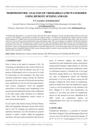
IJRET: International Journal of Research in Engineering and Technology eISSN: 2319-1163 | pISSN: 2321-7308
_______________________________________________________________________________________
Volume: 02 Issue: 08 | Aug-2013, Available @ http://www.ijret.org 514
MORPHOMETRIC ANALYSIS OF VRISHABHAVATHI WATERSHED
USING REMOTE SENSING AND GIS
P T Aravinda1
, H B Balakrishna2
1
Assistant Professor, Department of Civil Engg, Govt Engg College Ramanagara, Karnataka, India,
aravindapt@gmail.com
2
Professor, Department of Civil Engg, Bangalore Institute of Technology, Karnataka, India, balubit@gmail.com
Abstract
Vrishabhavathi Watershed is a constituent of the Arkavathi River Basin, Bangalore Urban and Ramanagara District and covers
an area of 381.465Km2
, representing seasonally dry tropical climate. To achieve the Morphometric analysis, Survey of India
(SOI) topomaps in 1:50000 scales are procured and the boundary line is extracted by joining the ridge points. This will serve as
study area or area of interest for preparing base map and thematic maps. The recent changes are updated with the help of Remote
sensing satellite data. The drainage map is prepared with the help of Geographical Information System tool and morphometric
parameters such as linear, aerial and relief aspects of the watershed have been determined. These dimensionless and dimensional
parametric values are interpreted to understand the watershed characteristics. From the drainage map of the study area dendritic
drainage pattern is identified. Strahler (1964) stream ordering method is used for stream ordering of the watershed. The drainage
density of the watershed is 1.697 km/km2
.
Index Terms: Morphometric analysis, Remote Sensing, GIS, SOI Topomap and Vrishabhavathi Watershed
--------------------------------------------------------------------***----------------------------------------------------------------------
1. INTRODUCTION
Water is known as the liquid for sustenance of life. All
living beings are depending on water, without which no life
exists on the earth. Earth has plentiful water due to the
presence of Hydrological cycle on it, but most of it is unfit
for living beings use and consumption. The study of the
watershed morphometric analysis provides the beneficial
parameters for the assessment of the ground water potential
zones, identification of sites for water harvesting structures,
water resource management, runoff and geographic
characteristics of the drainage system. Morphometry is the
measurement and mathematical analysis of the configuration
of the earth's surface, shape, dimension of its landforms
(Clarke, 1966). The Morphometric analysis consists of
linear, Aerial and relief aspects.
For the present study Remote Sensing (Lillisand Thomas,
2002) and Geographical Information System (GIS) will be
used as tools for managing and analyzing the spatially
distributed informations. Arc GIS and QGIS are powerful
softwares to analyze, visualize, update the geographical
information, and create quality presentations that brings the
power of interactive mapping and analysis. Many
researchers have done morphometric analysis using Remote
Sensing and GIS technique. (Shakil Ahmad et al., 2012) has
used Geoinformatics for assessing the morphometric control
on hydrological response at watershed scale in the upper
Indus Basin. (Sangita Mishra et al., 2010) has presented a
case study of Morphometric analysis and Watershed
prioritization of Tel river using Remote sensing and GIS
technique. (Vandana M, 2012) carried out morphometric
analysis for Kabini River basin and morphometric analysis
is used as a tool for prioritization of sub watershed in the
basin. (Magesh N S, 2013) used Geoinformatics for
extraction of river basin and carried out morphometric
analysis for that extracted river basin. (Balakrishna H B,
2008) carried out morphometric analysis for
Tippagondanahalli River basin for prioritization of sub
watersheds.
2. STUDY AREA
Vrishabhavathi Watershed is a constituent of Arkavathi
River Basin, Bangalore Urban and Ramanagara District and
covers an area of 381.465 Km2
lying between latitudes 120
441
3711
to 130
21
3111
N and longitudes 770
231
1411
to 770

_______________________________________________________________________________________
Volume: 02 Issue: 11 | Nov-2013, Available @ http://www.ijret.org 515
341
5911
E. Vrishabhavathi River is originated from Peenya
industrial area with an altitude of 930.250 m above mean
sea level. As per the data normal annual rainfall received by
the study area is 831mm. The geology of the study area is
characterized by the granite gneiss. Fig 1 shows the
Location Map of the Study area.
Fig-1: Location Map of Study area
3. METHODOLOGY
For the study outlet is taken at Vrishabhavathi Reservoir
situated at Byramangala village of Ramanagara Taluk,
Ramanagara District. The Fringe point is observed at hillock
of Peenya industrial area. A common task in hydrology is to
delineate a watershed from a topographic map. To trace the
boundary, one should start at the outlet Vrishabhavathi
Reservoir and then draw a line away on the left bank,
maintaining it always at right angles to the contour lines.
(The line should not cross the drainage paths) Continue the
line until it is generally above the headwaters of the stream
network. Return to the outlet and repeat the procedure with a
line away from the right bank. The two lines should join to
produce the full watershed boundary. The Digital Elevation
Model (DEM) of the study area is generated using ArcGIS
software. This helps in drawing the exact boundary line of the
study area. The base map is prepared using SOI toposheet
number 57H/5, 57H/6, 57H/9 and 57G/12 on 1:50,000 scale.
The Topomaps are scanned and projected for delineating the
required features. The Digitized maps are updated with the
help of satellite imagery using QGIS and ArcGIS softwares.
It consists of various features like the road network,
settlements, water bodies, Vrishabhavathi River, canals etc.
The South Western railway line passes through the study area
from Mysore to Bangalore is delineated from the toposheet.
The Bangalore-Mysore Highway and Tavarekere-
Konanakunte road networks are delineated from the
toposheet for the study area. The major settlements in the
present study area such as Kengeri railway station and
Hejjala Railway station are also delineated from the
toposheet. The information content of this map is used as a
baseline data to finalize the physical features of other
thematic maps. Since the topo sheets are very old all the
features like roads, railways, settlements etc are updated with
the help of recent rectified and scaled satellite imageries of
the area. Fig.2 shows Base map of Vrishabhavathi
Watershed.
Fig-2: Base map of Vrishabhavathi Watershed
The drainage map prepared from the toposheet forms the base
map for the preparation of thematic maps related to surface
and groundwater. All the streams, Vrishabhavathi River,

_______________________________________________________________________________________
tributaries and small stream channels shown on the toposheet
are extracted to prepare the drainage map.
The study area is a first, second, third, fourth, fifth and sixth
order streams and Vrishabhavathi River are present. The
present study area dendrite drainage patron is present. The
flowing of water is tamed through construction of number of
tanks and channels. Fig-3 shows Drainage map of
Vrishabhavathi Watershed.
Fig-3: Drainage map of the Vrishabhavathi Watershed
4. MORPHOMETRIC ANALYSIS
Morphometric analysis, which is all about exploring the
mathematical relationships between various stream
attributes, used to compare streams and to identify factors
that may be causing differences. The term Morphometry is
derived from a Greek word, where “morpho” means earth
and “metry” means measurement, so together it is
measurement of earth features. This is an important factor
for planning any watershed development.
Morphometric analysis also provides description of physical
characteristics of the watershed which are useful for
environmental studies, such as in the areas of land use
planning, terrain elevation, soil conservation and soil
erosion.
Morphometric analysis for the present study is grouped into
three classes such as linear aspects, areal aspects and relief
aspects.
4.1 Linear Aspects
Linear aspects include the measurements of linear features
of drainage such as stream order, bifurcation ratio, stream
length, stream length ratio, length of overland flow etc. The
linear characteristics of the drainage basin are discussed
below. (Ven Tee Chow, 1964)
4.1.1 Stream orders
The first step in drainage basin analysis is disignation of
stream osders, following a system introduced into the United
States by Horton (1956) and slightly modified by
Strahler(1964). Assuming that one has available drainage
network map including all intermittent and permanenet flow
lines located in clearly defined valleys, the smallest fingertip
tributaries are designated oreder 1. (Fig 4). Where two first
oredr channels join , a channel segment of oredr 2 is found.
Fig-4: Stream order Map of Vrishabhavathi Watershed

_______________________________________________________________________________________
Where two of order 2 joins, segment of order 3 is formed;
and so forth. The trunk stream through which all discharge
of water and sediment passes is therefore the stream
segment of highest order. Usefulness of the stream order
system depends on the premise that, on the average, if a
sufficiently large sample is treated, order number is directly
proportional to size of the contributing watershed, to
channel dimensions and to stream discharge at that place in
the system. Because order number is dimensionless, two
drainage networks differing greatly in linear scale can be
compared with respect to corresponding points in their
geometry through use of order number. After the drainage
network elements have been assigned their order numbers,
the segments of each order are counted to yield the number
Nu of segments of the given order u.
4.1.2 Bifurcation Ratio
It is obvious that the number of stream segments of any
given order will be fewer than for the next lower order but
more numerous than for the next higher order. The ratio of
number of segments of a given order Nu to the number of
segments of the higher order Nu+1 is termed the bifurcation
ratio Rb:
Rb =
Nu
Nu+1
The bifurcation ratio will not be precisely the same from one
order to the next, because of chance variations in watershed
geometry, but will tend to be a constant throughout the
series. Bifurcation ratio characteristically ranges between 3
and 5 for watersheds in which the geologic structures do not
distort the drainage pattern. The theoretical minimum
possible value of 2 is rarely approached under natural
conditions. Because the bifurcation ratio is a dimensionless
parameter, and because drainage systems in homogeneous
materials tend to display geometrical similarity, it is not
surprising that the ratio shows only a small variation from
region to region. Abnormally high bifurcation ratios might
be expected in regions of steeply dipping rock strata where
narrow strike valleys are confined between hogback ridges.
Average bifurcation ratio is calculated for the watershed as
3.84 (Table-1). Plotting the number of stream segments for
each stream order on logarithmic scale and stream order on
x-axis (Fig- 4) reveals a good relationship between them.
Fig-4: Regression of Stream order on Number of
stream segments
4.1.3 Stream Lengths
Mean stream length Lu of a stream channel segment of
order u is a dimensional property revealing the characteristic
size of components of a drainage network and its
contributing basin surfaces. Channel length is measured
with the help of ArcGIS and QGIS softwares directly from
the Stream Order map. To obtain the mean stream length of
channel Lu of order u, the total length is divided by the
number of stream segments Nu of that order, thus:
Lu =
Lu
N
i=1
Nu
Generally, The Lu increases with increase of order number.
It can be seen from Table 1, that the mean length of channel
segments of a given order is more than that of the next
higher order. The total number of all stream segments Nu in
a stream order, total stream length Lu in stream order u,
mean stream length for the watershed are calculated and is
shown in Table-2. Fig-5 shows that there is linear
relationship between mean stream length and stream order.
Steam length ratio
Stream length ratio (RL) is defined as the average length of
stream of any order to the average length of streams of the
next lower order and it is expressed as;
𝑅 𝐿 =
𝐿 𝑢
𝐿 𝑢−1
1
10
100
1000
1 2 3 4 5 6
StreamSegment
Stream Order

_______________________________________________________________________________________
Horton postulated that, the length ratio tends to be constant
throughout the successive orders of the stream.
Fig. 5 Regression of stream order on mean stream length
4.1.4 Length of overland flow
Horton defined length of overland flow L0 as the length of
flow path, projected to the horizontal, nonchannel flow from
a point on the drainage divide to a point on the adjacent
stream channel. He noted that length of overland flow is one
of the most important independent variables affecting both
the hydrologic and physiographic development of drainage
basins. During the evolution of the drainage system, L0 is
adjusted to a magnitude appropriate to the scale of the first
order drainage basins and is approximately equal to one half
the reciprocal of the drainage density. The shorter the
length of overland flow, the quicker the surface runoff from
the streams. For a present study Length of Overland Flow is
0.295.
4.1.5 Drainage pattern
In geomorphology, a drainage system is the pattern formed
by the streams, rivers, and lakes in a particular drainage
basin. They are governed by the topography of the land,
whether a particular region is dominated by hard or soft
rocks, and the gradient of the land. Geomorphologists and
hydrologists often view streams as being part of drainage
basins. A drainage basin is the topographic region from
which a stream receives runoff, through flow, and
groundwater flow. Drainage basins are divided from each
other by topographic barriers called a watershed. A watershed
represents all of the stream tributaries that flow to some
location along the stream channel. The number, size, and
shape of the drainage basins found in an area varies and the
larger the topographic map, the more information on the
drainage basin is available. A drainage system is described as
accordant if its pattern correlates to the structure and relief of
the landscape over which it flows. Following are the some of
the drainage patterns in the world.
Dendritic drainage pattern: Dendritic drainage systems
are the most common form of drainage system. In a
dendritic system, there are many contributing streams
(analogous to the twigs of a tree), which are then joined
together into the tributaries of the main river (the branches
and the trunk of the tree, respectively). They develop where
the river channel follows the slope of the terrain. Dendritic
systems form in V-shaped valleys; as a result, the rock types
must be impervious and non-porous.
Parallel drainage pattern: A parallel drainage system is a
pattern of rivers caused by steep slopes with some relief.
Because of the steep slopes, the streams are swift and
straight, with very few tributaries, and all flow in the same
direction. This system forms on uniformly sloping surfaces,
for example, rivers flowing southeast from the Aberdare
Mountains in Kenya. Parallel drainage patterns form where
there is a pronounced slope to the surface. A parallel pattern
also develops in regions of parallel, elongate landforms like
outcropping resistant rock bands.
Trellis drainage pattern: The geometry of a trellis
drainage system is similar to that of a common
garden trellis used to grow vines. As the river flows along a
strike valley, smaller tributaries feed into it from the steep
slopes on the sides of mountains. These tributaries enter the
main river at approximately 90 degree angles, causing a
trellis-like appearance of the drainage system. Trellis
drainage is characteristic of folded mountains, such as
the Appalachian Mountains in North America.
Rectangular drainage pattern: Rectangular drainage
develops on rocks that are of approximately uniform
resistance to erosion, but which have two directions
of jointing at approximately right angles. The joints are
usually less resistant to erosion than the bulk rock so erosion
0.1
1
10
100
1 2 3 4 5 6
MeanStreamlength
Stream Order

_______________________________________________________________________________________
tends to preferentially open the joints and streams eventually
develop along the joints. The result is a stream system in
which streams consist mainly of straight line segments with
right angle bends and tributaries join larger streams at right
angles.
Radial drainage pattern: In a radial drainage system, the
streams radiate outwards from a central high
point. Volcanoes usually display excellent radial drainage.
Other geological features on which radial drainage
commonly develops are domes and laccoliths. On these
features the drainage may exhibit a combination of radial
patterns. (Subramanya K, 2012)
The drainage pattern for the present study area is dendritic.
The drainage pattern shows well integrated pattern formed
by a main stream with its tributaries branching and
rebranching freely in all direction. The dendritic pattern of
drainage indicates that the soil is semi pervious in nature.
Table 1 Linear morphometric parameters of
Vrishabhavathi watershed
Str
Ord
No of
Segme
nts
Total
length
Bifurcation
Ratio
Mean
length
Length
Ratio
1 651 372.603 0.572
2 126 121.225 5.166 0.962 1.681
3 27 70.629 4.666 2.616 2.719
4 8 51.272 3.375 6.409 2.449
5 2 19.307 4.000 9.654 1.506
6 1 12.537 2.000 12.537 1.298
4.2 Areal aspects
Areal aspects (Au) of a watershed of given order u is defined
as the total area projected upon a horizontal plane
contributing overland flow to the channel segment of the
given order and includes all tributaries of lower order. The
watershed shape has a significant effect on stream discharge
characteristics, for example, the elongated watershed having
a high bifurcation ratio can be expected to have alternated
flood discharge. But on the other hand, the round or circular
watershed with a low bifurcation ratio may have a sharp
peak flood discharge.
The shape of a watershed has a profound influence on the
runoff and sediment transport process. The shape of the
catchment also governs the rate at which water enters the
stream. The quantitative expression of watershed can be
characterised as form factor, circularity ratio, and elongation
ratio.
4.2.1 Form factor
Horton defines the form factor Rf as a dimensionless ratio
of watershed area (A) to the square of the length of the
watershed (L). The value of form factor would always be
less than 0.7854 (for a perfect circular watershed). The
watershed with higher form factor are normally circular and
have high peak flows for shorter duration, whereas
elongated watershed with lower values of form factor have
low peak flows for longer duration. For the present study
area form factor is 0.327.
Rf =
A
L2
Where Rf is the form factor, L is the total length of
watershed and A is the total area of watershed.
4.2.2 Circularity ratio
Circularity ratio is the ratio between the area of watershed to
the area of circle having the same circumference as the
perimeter of the watershed (Miller, 1953). The value ranges
from 0.2 to 0.8, greater the value more is the circularity
ratio. It is the significant ratio which indicates the stage of
dissection in the study region. Its low, medium and high
values are correlated with youth, mature and old stage of the
cycle of the tributary watershed of the region, and the value
obtained. For the present study area circularity ratio is
obtained as 0.492.
Rc =
4πA
P2
Where Rc = Circularity ratio, A = Watershed area, P =
Perimeter of watershed.
4.2.3 Elongation ratio
Elongation ratio is the ratio between the diameter of the
circle having the same area as the watershed and maximum
length of the basin (Schumn, 1956).
Smaller form factor shows more elongation of the basin.
The watershed with higher form factor will have higher peak

_______________________________________________________________________________________
flow for shorter duration. Whereas elongated watershed with
low form factor, will have a flatter peak of flow for longer
duration.
𝑅 𝑒 =
2
𝐴
𝜋
𝐿
Where Re is the Elongation ratio, L is the total length of
watershed and A is the total area of watershed.
The value of elongation ratio ranges from 0.4 to 1, lesser the
value, more is the elongation of the watershed. For the
present study area elongation ratio is calculated as 0.645.
4.2.4 Drainage density
Drainage density is the other element of drainage analysis
which provides a better quantitative expression to the
dissection and analysis of land forms, although a function of
climate, lithology, structures and relief history of the region,
etc. can ultimately be used as an indirect indicator to explain
those variables, as well as the morphogenesis of landform.
Drainage density (Dd) is one of the important indications of
the linear scale of landform elements in stream eroded
topography. It is defined as the total stream length of all
stream order to the total area of watershed. The drainage
density, which is expressed as km/Sq.km, indicates a
quantitative measure of the average length of stream channel
area of the watershed. Drainage density varies inversely
with the length of the overland flow, and therefore, provides
at least some indication of the drainage efficiency of the
basin. Drainage density is mathematically expressed as:
𝐷𝑑 =
𝐿 𝑢
𝑁
𝑖=1
𝐴
Where 𝐿 𝑢
𝑁
𝑖=1 = Cumulative length of all streams (km)
A = Area of watershed (Sq. km)
The measurement of drainage density provides a hydrologist
or geomorphologist with a useful numerical measure of
landscape dissection and runoff potential. On a highly
permeable landscape, with small potential for runoff,
drainage densities are sometimes less than 1 kilometer per
square kilometer. On highly dissected surfaces densities of
over 500 kilometers per square kilometer are often reported.
Closer investigations of the processes responsible for
drainage density variation have discovered that a number of
factors collectively influence stream density. These factors
include climate, topography, soil infiltration capacity,
vegetation, and geology. The low value of drainage density
influences greater infiltration and hence the wells in this
region will have good water potential leading to higher
specific capacity of wells. In the areas of higher drainage
density the infiltration is less and surface runoff is more.
The drainage density can also indirectly indicated
groundwater potential of an area, due to its surface runoff
and permeability. The value obtained (drainage density) was
1.697 Km/Sq.km for the present study. From this, it was
inferred that the area is very coarser watershed. The
drainage density obtained for the study area is low
indicating that the area has highly resistant or highly
permeable sub-soil material.
4.2.5 Constant of channel maintenance
The inverse of drainage density is the constant of channel
maintenance (C). It indicates the number of Sq.km of
watershed required to sustain one linear Km of channel.
C =
1
Dd
It not only depends on rock type permeability, climatic
regime, vegetation, relief but also as the duration of erosion
and climatic history. The constant of channel maintenance is
extremely low in areas of close dissection.
4.2.6 Stream frequency
Stream frequency may be expressed by relating the number
of stream segments to the area drained. In other words,
Stream frequency is the total number of stream segments in
a watershed divided by the area of the watershed. Horton,
1932) introduced stream frequency or channel frequency as
number of stream segments per unit area. For the present
study, the stream frequency is 1.67.
𝑆𝑓 =
𝑁𝑢
𝑁
𝑖=1
𝐴
Where 𝑁𝑢
𝑁
𝑖=1 = Total no. of stream segments
A = Total area of watershed (Sq. km).

_______________________________________________________________________________________
4.3 Relief aspects
Relief aspects are an important factor in understanding the
extent of denudational process undergone within the
catchment and it is indicator of flow direction of water.
4.3.1 Watershed relief
Watershed relief is the difference in elevation between the
remotest point in the water divide line and the discharge
point of the watershed.
H= (Difference in elevation of the highest point of
watershed) - (Difference in elevation of the watershed
outlet)
The difference in elevation between the remotest point and
discharge point is obtained from the available contour map.
The highest relief is formed in watershed at an elevation of
930.250 m above mean sea level. The lowest relief was
obtained at the Byramangala Reservoir at an elevation of
696.470 m above msl. The overall relief calculated for the
watershed was 0.234 km.
4.3.2 Relief ratio
Schumm (1956) defined relief ratio as the total watershed
relief to the maximum length of the watershed. The relief
ratio for the watershed was obtained as 0.0068. The relief
ratio increases overall the sharpness of the drainage basin
and it is an indicator of intensity process operating as the
shape of the watershed.
Rh =
H
L
Where Rh= Relief ratio
Where H = Total catchment relief (km)
L = Maximum length of catchment (km)
4.3.3 Relative relief
Relative relief is defined as the ratio of the maximum
watershed relief to the perimeter of the watershed. It is
computed as 0.0054 using the equation
Rr =
H
P
Where R r = Relative relief; H = Maximum relief (km); P =
Perimeter (km)
4.3.4 Ruggedness number
Strahler (1964) defined Ruggedness number is the product
of the watershed relief and drainage density and usually
combines slope steepness with its length. High values of the
ruggedness number in the watershed area because both the
variables like relief and drainage density are enlarged. It is
computed as 0.397 using the equation.
𝑅 𝑛 = 𝐻𝐷𝑑
Where Rn = Ruggedness number, H = Watershed relief
(km), Dd = Drainage density km/Km2
Table 6 shows different morphometric parameters of
Vrishabhavathi watershed.
Table -2: Different Morphometric Parameters of
Vrishabhavathi Watershed
Watershed Parameters Units Values
Watershed Area Sq.km 381.465
Perimeter of the Watershed km 98.628
Highest Stream Order No. 6
Length of watershed km 34.150
Maximum width of Watershed km 20.373
Cumulative Stream Segment km 815
Cumulative Stream Length km 647.573
Length of overland flow km 0.295
Drainage Density Km/Sq.km 1.697
Constant of Channel
Maintenance
Sq.km/Km 0.589
Stream Frequency No/Sq.km 2.136
Bifurcation Ratio 3.84
Length Ratio 1.931
Form Factor 0.327
Circularity Ratio 0.492
Elongation Ratio 0.645
Total Watershed Relief km 0.234
Relief Ratio 0.0068
Relative Relief 0.0054
Ruggedness Number 0.397
5. CONCLUSION
From the quantitative study, it is seen that the basin forms
the dendritic pattern of drainage. Average bifurcation ratio is
calculated for the watershed as 3.84. The value of Rb in the
present case indicates that watershed has suffered less
structural disturbance and the watershed may be regarded as
the elongated one. Drainage density reflects land use and
affects the infiltration and the watershed response time
between the precipitation and discharge. For the present
study the drainage density is evaluated to be 1.697
Km/Sq.km which indicates that the area is of coarser in
nature.

_______________________________________________________________________________________
The circularity ratio for the watershed is 0.492, which
indicates mature nature of topography. Its low, medium and
high values area correlated with youth, mature and old stage
of cycle of tributary watershed of the region. The elongation
ratio is 0.645, which indicates that the watershed is
elongated. The stream frequency obtained for the study area
is 2.136 No./Sq.km. So it is classified under the class of low
drainage density, leading to higher bifurcation ratio in to the
soil. On the whole, the watershed has a total relief of 0.234
Km. The relief aspect shows that the watershed has enough
slope for runoff to occur from the source to the mouth of
watershed. The morphometric analysis results in
dimensionless parameters for the watershed. This helps to
compare the watershed with the neighbouring watersheds
and to make decision for constructing hydraulic structures to
combat erosion.
6. REFERENCES:
1.Balakrishna H B (2008). Spatial decision support system
for watershed management using Remote Sensing and
Geographic Information System, Ph.D. Thesis, UVCE,
Department of Civil Engineering, Bangalore University.
2.Clarke J J (1966), Morphometry from map, Essays in
geomorphology. Elsevier Publishing Company, New York p
235-274.
3.Horton R E (1945) Erosional development of streams and
their drainage basins: Quantitative Morphology, Bull
Geological Society of America 56:275 361.
4.Lillesand Thomas, Kifer M, Ralph W, (2002) Remote
Sensing and Image Interpretation, 4th Ed., John Wiley &
Sons, Inc. New York.
5.Magesh N S, Jitheshlal K V and Chandrasekar N(2013)
Geographical information system-based morphometric
analysis of Bharathapuzha river basin, Kerala, India. Appl
Water Sci (2013) 3:467–477.
6.Sangita Mishra.S, Nagarajan.R (2010) Morphometric
analysis and prioritization of subwatersheds using GIS and
Remote Sensing techniques: a case study of Odisha, India.
International journal of geomatics and geosciences Volume
1, No 3, 2010.
7.Schumm S. A., (1956) Evolution of Drainage Systems
and Slopes in Bad Lands at Perth, Amboy, New Jersey,
Bull. Geol. Soc. Amec., 67, pp. 597-646.
8.Shakil Ahmad et al (2012) Geoinformatics for assessing
the morphometric control on hydrological response at
watershed scale in the Upper Indus Basin. J. Earth Syst. Sci.
121, No. 3, June 2012, pp. 659–686
9.Strahler A N (1964) Quantitative Geomorphology of
Drainage Basin and Channel Networks. Handbook of
Hydrology (edited by Ven Te Chow) Mc Graw Hill,Section
4-11.
10.Subramanya, K., (2012) A Text Book of Engineering
Hydrology, Tata McGraw-Hill Publications, New Delhi.
11.Vandana M (2013) Morphometric analysis and watershed
prioritization. A case study of Kabini River Basin, Wayanad
District, Kerala, India. Indian Journal of Geo Marine
Sciences. Vol 42(2), April 2013, pp 211- 222.
12.Ven Te Chow (1964), Handbook of applied Hydrology,
McGraw-Hill Book Company.
BIOGRAPHIES:
ARAVINDA P T
Assistant Professor, Department of Civil
Engg, Govt Engg College Ramanagara,
Karnataka, India
Main research areas: Watershed
management, remote sensing and GIS.
Email: aravindapt@gmail.com
Dr.H B BALAKRISHNA
Professor, Department of Civil Engg,
Bangalore Institute of Technology,
Karnataka, India, Main research areas:
Watershed management, remote sensing
and GIS. Email: balubit@gmail.com

Morphometric analysis of vrishabhavathi watershed using remote sensing and gis

Recommended

Recommended

More Related Content

What's hot

What's hot (20)

Viewers also liked

Viewers also liked (17)

Similar to Morphometric analysis of vrishabhavathi watershed using remote sensing and gis

Similar to Morphometric analysis of vrishabhavathi watershed using remote sensing and gis (20)

More from eSAT Journals

More from eSAT Journals (20)

Recently uploaded

Recently uploaded (20)

Morphometric analysis of vrishabhavathi watershed using remote sensing and gis