
Recommended
Recommended
More Related Content
Similar to Instructions 1. Using annual data on GDP from the U.S. Cens.docx
Similar to Instructions 1. Using annual data on GDP from the U.S. Cens.docx (11)
More from dirkrplav
More from dirkrplav (20)
Recently uploaded
Recently uploaded (20)
Instructions 1. Using annual data on GDP from the U.S. Cens.docx
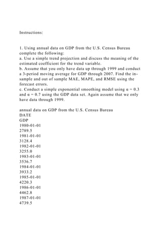
- 1. Instructions: 1. Using annual data on GDP from the U.S. Census Bureau complete the following: a. Use a simple trend projection and discuss the meaning of the estimated coefficient for the trend variable. b. Assume that you only have data up through 1999 and conduct a 3-period moving average for GDP through 2007. Find the in- sample and out of sample MAE, MAPE, and RMSE using the forecast errors. c. Conduct a simple exponential smoothing model using α = 0.3 and α = 0.7 using the GDP data set. Again assume that we only have data through 1999. annual data on GDP from the U.S. Census Bureau DATE GDP 1980-01-01 2789.5 1981-01-01 3128.4 1982-01-01 3255.0 1983-01-01 3536.7 1984-01-01 3933.2 1985-01-01 4220.3 1986-01-01 4462.8 1987-01-01 4739.5
- 3. 2006-01-01 13194.7 2007-01-01 13843.8 2. Complete the Forecasting for Tracway for mowers using the Tracway data. For this exercise, forecast industry sales as well as market share. Compare the moving average (3 month) method against Winter's method. Since we are forecasting mowers, think about which model you would expect to be more accurate. After working through the problems, go to Lesson 9: Individual Exercises 9 and answer the associated multiple choice questions. Forecasting for Tracway An important input to planning manufacturing capacity is a good forecast of sales. In reviewing the Tracway database, Henry Hudson is interested in forecasting sales for mowers and tractors in each marketing region. Although Henry has obtained expert opinions on sales forecasting using the Delphi process, he would like to generate time series forecasts for the next year for each product by region. Henry plans to then compare and incorporate the judgmental forecasts from the Delphi process to the quantitative forecasts developed via the Delphi process. Tracway data. See attached worksheet labeled (Tracway data)
- 4. Questions: Using annual data on GDP from the U.S. Census Bureau answer questions 1-6. 1. The trend analysis reveals A) no evidence of any clear trend either upward or downward.
- 5. B) an upward trend. C) an downward trend. D) a positive but insignificant coefficient for the trend variable. 2. According to the F-statistic we cannot reject the null hypothesis that R2 = 0 when using trend analysis. A) True B) False 3. When conducting a 3-period moving average for GDP through 2007 the out of sample Mean Absolute Error (MAE) is found to be approximately A) $682 B) $696 C) $1,043 D) none of the above 4. The moving average analysis shows forecasts that consistently underestimate actual GDP. A) True B) False 5. When using an exponential smoothing model for α = 0.3, the out of sample MAPE is ____________ and the within sample MAPE is ____________. A) 21.85%, 11.45% B) 20.62%, 8.35% C) 27.83%, 16.29% D) none of the above 6. The exponential smoothing forecast is more accurate at α = 0.7
- 6. than at α = 0.3. A) True B) False Complete the Forecasting for Tracway for mowers and answer questions 7-12. 7. Using the 3 month moving average for industry sales, which region is found to have the smallest MAE? A) North America B) South America C) Europe D) Pacific 8. Using Winter’s method for industry sales, which region is found to have the smallest RMSE? A) North America B) South America C) Europe D) Pacific 9. The MAPE reveals that the average forecast misses the target by 3.00% using Winter’s method in South America for industry sales. A) True B) False 10. Which statement most accurately reflects the meaning of the optimal smoothing constants found for industry sales in South America and Europe? A) The model misses the target by 1.00% using Winter’s
- 7. method. B) The model reacts slowly to changes in level, but quickly to trend and season for Winter's method. C) The model reacts right away to changes in level, but almost never reacts to trend for Winter's method. D) none of the above 11. Market share forecast errors are all smaller in comparison to sales which makes sense because one would not expect any region to have significant gains or losses in market share over the course of the 12 months forecasted in the models. A) True B) False 12. The regional sectors forecast for industry sales and market share are better using Winter's method which can be seen by the results for MAE and MAPE. A) True B) False Focus of the Final Paper This assignment focuses on how the management practices of planning, leading, organizing, staffing, and controlling are implemented in your workplace. If you are not currently working, you may use a previous employer. In this assignment, you must: · Analyze the application of these management concepts to your place of work; the paper will not simply be a report on the five functions in general. · Identify specific examples and explain of how each applies to the functions practiced in your place of work. Be sure to integrate vocabulary learned throughout this course
- 8. and citations from the text to support your analysis. The paper should be five to six pages in length and formatted according APA style guidelines as outlined in the Ashford Writing Center. Writing the Final Paper The Final Paper: 1. Must be five to six double-spaced pages in length, excluding the title and reference pages, and formatted according to APA style as outlined in the Ashford Writing Center. 2. Must include a title page with the following: 1. Title of paper 2. Student’s name 3. Course name and number 4. Instructor’s name 5. Date submitted 3. Must begin with an introductory paragraph that has a succinct thesis statement. 4. Must address the topic of the paper with critical thought. 5. Must end with a conclusion that reaffirms your thesis. 6. Must use at least five scholarly sources, including a minimum of three from the Ashford University Library, in addition to the course textbook. 7. Must document all sources in APA style, as outlined in the Ashford Writing Center. 8. Must include a separate reference page, formatted according to APA style as outlined in the Ashford Writing Center. Baack, D., Reilly, M., & Minnick, C., & (2014). The five functions of effective management(2nd ed.). San Diego, CA: Bridgepoint Education, Inc. Instructions: Download and read the Regression Experiment and answer the questions in part C of the document titled Analysis and Interpretation. After working through the problems, go to Lesson 8: Individual
- 9. Exercises 8 and answer the associated multiple choice questions. Regression Experiment: An Overview of Model Development and Interpretation THE DEMAND FOR ROSES A. The Market for Roses Roses have an almost universal identification with the act of sending flowers, and consequently, they are one of the major products that the retail florist sells either alone or as part of floral arrangements. The wholesale cut flower supplier must therefore be able to supply roses to retail florists. However, a number of factors have recently affected the growth in demand for roses. First, there has been a general breakdown of "old country social customs" such as the tradition of always sending flowers to funerals. Second, there has been a growth in demand for competing products, such as carnations and wild flowers, which live longer than roses. Likewise, there has been increased use by retailers of other flowers that are larger and require smaller quantities per arrangement. Also, in this context, there has been accelerated growth in the demand for green plants. Green plant sales only accounted for 22 percent of the total sales for the floral industry in 1975, but had jumped to 42 percent by 1984, and are predicted to rise above 50 percent in the 1990s. Third, the costs of growing roses have been increasing significantly.B. Developing a Demand Function (Model) for Roses Matthew’s and Sons is wholesale supplier of rose to retail florists in the Detroit metropolitan area. This firm is concerned with developing a model that will aid in forecasting rose sales (Qt) and developing appropriate strategies for the firm's operations. Data on Matthew’s rose sales over the past sixteen quarters was available from their monthly sales summaries. See Table 1 for data on variables that Matthew and Sons thought
- 10. would be key to their demand analysis. Price data for roses and carnations was available form Matthew and Sons' billing records; unemployment data for the Detroit area was available in the Michigan Manpower Review; information on births, deaths, and marriages ("flower events") was obtained from the Michigan Department of Health; average family income is available from the U.S. Department of Labor.C. Analysis and Interpretation 1. Your task is to use the data in Table 1 to develop a demand model for Matthew and Sons' sales of roses. It would be a great learning experience to try and do this on your own first, then use my suggestions below to compare your analysis to mine. Note: you should begin by including the price of roses (RosePr), the price of carnations (CarnatPr) and the trend variable (time) as well as a constant (i.e. an intercept). Then explain the expected sign (+, -, or ?) for each of those variables as well as any other variables you deem appropriate to include in your model. Finally, use multiple regression to estimate the coefficients for your model. 2. To what extent was multicollinearity a problem in choosing an appropriate model to estimate? Use theory and computer output to support your answer. 3. Run a regression using the following variables: price of roses (Rosepr), the price of carnations (CarnatPr), the trend variable (time), Births, Deaths, Wedding, Unemp, Income as well as a constant. Describe each variable coefficient as insignificant, significant at .10, significant at .05 or significant at .01 and whether you used a one- or two-tail test and why. What is the advantage of using Births, Deaths and Wedding instead of just Events? Would it be wise to include Events and also Births, Deaths and Wedding? 4. Interpret precisely the parameter (coefficient) associated
- 11. with the price of roses. 5. Calculate and interpret the price elasticity for roses. Using elasticity formula from iMBA 501: Ep=%change in dozen / %change in rosepr = Δdozen/ ΔQrosepr x mean rosepr/mean dozen = price coefficient x mean rosepr/mean dozen. 6. What level of substitutability exists between roses and carnations? Provide support for your answer. 7 What is the R2 of your model? Interpret its magnitude. 8. Is the apparent explanatory power of the model as indicated by the value of R2 statistically significant? Do the appropriate F-test to confirm or refute. 9. Interpret the coefficient on the trend variable. Why may such a result have occurred? 10. Suppose the florists believe that first-quarter sales are greater than sales in any other quarter. Create and define a variable(s) that will allow you to test this hypothesis. Re- estimate the equation with your new variable. Are the florists correct about first-quarter sales? 11. What are some of the shortcomings of this model? What variable(s) may have been omitted from this model? Table 1 Demand for Roses Data You can copy this data and paste directly in Excel. Births, Deaths, and Weddings are flower events. Events = Births + Deaths + Weddings. CarnatPr = the price of a dozen carnations.
- 12. RosePr = the price of a dozen roses. Dozen = the number of roses sold (in dozens). Time = trend variable. Unemp = unemployment rate. Income = Average family income ($100 units) Date Births CarnatPr Deaths Events Wedding RosePr Dozen Time Unemp Income 1992.Q3 19284 18.49 8819 40022 11919 32.26 11484 1 7.6 173.36 1992.Q4 18062 17.85 9334 36996 9600 32.54
- 17. 15 6.2 195.67 1996.Q3 14769 18.53 8324 33907 10814 33.69 5872 16 5.4 208.00 Questions: Run a regression using the following variables: price of roses (Rosepr), the price of carnations (CarnatPr), the trend variable (time), Births, Deaths, Wedding, Unemp, Income as well as a constant. Answer questions 1-10 based on this model. 1. Which of the following is true of the expected coefficients in the model? A) Births, deaths, wedding, price of carnations, and income are expected to be positive and the price of roses and unemployment are expected to be negative. B) Births, deaths, wedding, and income are expected to be positive and the price of roses, price of carnations, and
- 18. unemployment are expected to be negative. C) Price of carnations and income are expected to be positive and births, deaths, wedding, the price of roses and unemployment are expected to be negative. D) none of the above 2. The price elasticity for roses is approximately A) -10.9 B) -3.7 C) -1.9 D) none of the above 3. The cross price elasticity for roses and carnations is approximately A) 2.0 B) 3.2 C) 4.5 D) none of the above 4. The coefficient associated with the price of roses can be interpreted as follows: For every $1 increase in the price of a dozen roses, there are 2526.23 dozen less sold holding all other variables constant. A) True B) False 5. The estimated coefficient for wedding is found to be approximately A) 0.47 and is insignificant. B) 0.12 and is significant at the .01 level. C) -0.29 and is insignificant. D) none of the above.
- 19. 6. The estimated coefficient for Deaths is found to be insignificant and therefore should be dropped from the regression model. A) True B) False 7. Which of the following pairs of variables exhibits the highest degree of multicollinearity? A) wedding and events B) births and events C) income and unemployment D) none of the above. 8. Which of the following statements best represents the interpretation of the R2 for this model? A) The variables included in the model explain 91.9% of the variation in the number of dozens of roses sold. B) The variables included in the model explain 97.9% of the variation in the number of dozens of roses sold. C) The variables included in the model explain 95.5% of the variation in the number of dozens of roses sold. D) none of the above 9. Which of the following statements best represents the interpretation of the explanatory power of the R2 for this model? A) The F-critical is greater than the F-statistic so we can reject the null hypothesis of no explanatory power for the model. B) The F-critical is less than the F-statistic so we cannot reject the null hypothesis of no explanatory power for the model. C) The F-critical is greater than the F-statistic so we cannot reject the null hypothesis of no explanatory power for the
- 20. model. D) none of the above 10. According to the coefficient associated with the trend variable, the number of dozens of roses sold was decreasing at a rate of 472.67% per quarter more than could be explained by changes in the other variables. A) True B) False Suppose the florists believe that first-quarter sales are greater than sales in any other quarter. Create and define a variable(s) that will allow you to test this hypothesis. Re-estimate the equation with your new variable and answer question 11. 11. The florists are correct about the first-quarter sales being greater than sales in any other quarter. A) True B) False 12. A potential shortcoming of this model could be A) the high degree of substitutability between the price of roses and the price of carnations B) multicollinearity between sales of roses and the price of carnations C) an omitted variable such as green plant price D) none of the above 1. Pearson Correlation cannot be used to identify non-linear relationships between two variables.
- 21. A) True B) False 2. Regression cannot be used to identify non-linear relationships between two variables. A) True B) False 3. Suppose you have a regression model that depicts the relationship between sales in dollars (S) and the price of the product in dollars (P) such that S = 10 - 2P. Which of the following is the correct interpretation of the price coefficient (i.e., -2)? A) A $1 increase in price will decrease sales by $2. B) A $1 increase in sales will occur if there is a $2 decrease in price. C) A 1% increase in price will cause a 2% decrease in sales. D) A 1% increase in sales will be caused by a 2% decrease in price. 4. Suppose you have a regression model that depicts the relationship between sales in dollars (S) and the price of the product in dollars (P) such that log(S) = 10 - 2(logP). Which of the following is the correct interpretation of the price coefficient (i.e., -2)? A) A $1 increase in price will decrease sales by $2. B) A $1 increase in sales will occur if there is a $2 decrease in price. C) A 1% increase in price will decrease sales by 2%. D) A 1% increase in sales will result from a 2% decrease in price. Situation 8.1:
- 22. A chemist employed by a pharmaceutical company has developed a muscle relaxant. She took a sample of 14 people suffering from extreme muscle constriction. She gave each a vial of the liquid drug and recorded the time to relief (measured in seconds)for each. She then estimated a regression model to this data and found the following: Relief = 1283 (3.65) - 25.22Dose (2.92) - 0.86DoseSquared (2.13) where numbers in parentheses are t-statistics for the corresponding variable coefficient. 5. The chemist ask you to determine if the there is a significant relationship between dose and time to relief. Using a one-tail test, your best answer would be: A) Given the results provided, dose is significant at .01 level. B) Given the results provided, dose is significant at the .05 level. C) Given the results provided, dose is significant at the .10 level. D) Given the results provided, dose does not significantly affect time to relief. 6. Suppose the chemist decides to determine if there is a quadratic effect (e.g. DoseSquared). Should the chemist use a one-tail or two-tail test? A) A one-tail since the effect of increasing the dosage will eventually taper off so expect dose squared to be negative. B) A one-tail test since the effect of increasing the dosage will be to accelerate time to relief so expect sign of dose squared is positive. C) A two-tail test since we do not know what effect an increased dosage will have so do not know sign to expect for dose squared. D) One could select either a one-tail or two-tail test as long as test at alpha = 0.01.
- 23. 7. The chemist concludes that there is a quadratic effect (Dose- squared) for the muscle relaxation medication. This conclusion is appropriate using a two-tail test and alpha = .05. A) True B) False 8. A dummy variable is used when: A) Two variables are collinear. B) The model is non-linear C) The variable is categorical or qualitative. D) The preferred variable is missing and you must use a proxy variable. You are hired by a major refrigerator manufacturer to estimate the demand for their refrigerators. You use the following independent variables in this effort. i. Population (POP), age 21-35, in thousands.
- 24. ii. Housing starts (H), in thousands. iii. Refrigerator price index (P). iv. Disposable personal income per capita (Y), in thousands of dollars. v. Advertising expenditures (A), in thousands of dollars. vi. Replacement trend (R), a replacement probability function constructed from prior refrigerator sales, based on a 16-year average refrigerator life, and average age of refrigerators in market area. Quarterly data for the years 1997 through 2002 were used to run the regression on refrigerator sales (in thousands). The results are described in Tables 1 and 2 below. TABLE 1: Regression Results Variable Coefficient t-stat POP +0.045 1.41 H +0.657 3.13 P -1579.0 2.21 Y +2254.0 1.56 A +67.5
- 25. 2.74 R +0.756 4.85 CONSTANT -1245.0 1.11 R2 = .67 Adjusted R2 = .59 F = 2.75 TABLE 2:Correlation Matrix Variables Correlation Variables Correlation Variables Correlation POP,H .844 H,P .356 P,A .055 POP,Y .767 H,Y .904 P,R -.005 POP,R -.003
- 26. H,A .015 Y,A .805 POP,P .450 H,R .120 Y,R .225 POP,A .674 P,Y .856 A,R .022 9. Assuming that a one-tail test is appropriate for all coefficients and a significance level of .05, which of the variables in the model are significant (exclude constant or intercept from consideration)? A) R,H,A B) R,H,A,P C) R,H,A,P,Y D) R,H,A,P,Y,POP 10. What problem can be caused by multicollinearity? A) The inability to isolate the distinct effects of the related independent variables. B) Smaller than expected p-values leading to misinterpretations. C) Smaller than expected standard errors leading to wrong conclusions. D) Significant t-values and a high R-squared.
- 27. 11. Which of the following is the best example of the potential issues associated with multicollineary? A) Adjusted R-squared is less than R-squared. B) H and R have a low correlation but both have significant coefficients. C) POP and Y are correlated and both have insignificant coefficients. 12. Suppose you check on seasonality in the sales of refrigerators by creating the following variables: Q1 = 1 if first quarter, 0 otherwise; Q2 = 1 if second quarter, 0 otherwise; and Q3 = 1 if third quarter, 0 otherwise. The coefficient for Q2 equals +0.5 and is statistically significant and Q4 is the “omitted” category. Interpret Q2. A) There are, on average, 500 more refrigerators sold in the second quarter, holding constant the other variables. B) There are, on average, 500 more refrigerators sold in the second quarter than the first quarter, holding constant the other variables. C) There are, on average, 500 more refrigerators sold in the second quarter than the third quarter, holding constant the other variables. D) There are, on average, 500 more refrigerators sold in the second quarter than the fourth quarter, holding constant the other variables. 1. When testing the equality of population variances, the test statistic is the ratio of the sample variances (or equivalently, the ratio of the squared standard deviations). A) True
- 28. B) False 2. When we test for differences between the means of independent populations, we can only use a one-tail test. A) True B) False 3. The sample size in each independent sample must be the same if we are to test for differences between means. A) True B) False 4. A statistics professor wanted to test whether the grades on a statistics quiz were the same for the online and resident MBA students. The professor took a random sample of 15 students from each course and is going to conduct a test to determine if the VARIANCES in the grades for online and resident MBA students are equal. For this test, the professor should use a t-test with related or matched samples. A) True B) False
- 29. Situation 6.1.1: Do Japanese managers have different motivation levels than American managers? A randomly selected group of each were administered the Sarnoff Survey of Attitudes Toward Life (SSATL), which measures motivation for upward mobility. Higher scores indicate more motivation. The SSATL scores are summarized below. Japanese Mgrs American Mgrs Sample Size 211 100 Mean SSATL Score 65.75 79.83 Population Std. Deviation 11.07 6.41 5. What is the appropriate null and alternative hypothesis for testing the question posed in Situation 6.1.1? A) µJ - µA ≥ 0; H1:µJ - µA < 0 B) µJ - µA ≤ 0; H1: µJ - µA > 0 C) µJ - µA = 0; H1: µJ - µA ≠ 0 - - 6. Given the following results generated in Excel, are the variances in the sample of Japanese managers different than the variances in the sample of U.S. managers at the .05 level of significance?
- 30. Data Level of Significance 0.05 Population 1 Sample Sample Size 211 Sample Standard Deviation 11.07 Population 2 Sample Sample Size 100 Sample Standard Deviation 6.41 Intermediate Calculations F-Test Statistic 2.982491 Population 1 Sample Degrees of Freedom 210 Population 2 Sample Degrees of Freedom 99 Two-Tailed Test Lower Critical Value 0.719629 Upper Critical Value 1.419014 p-Value 6.01E-09
- 31. A) Yes, there are significant differences in the sample variances. B) No, there are no significant differences in the sample variances. 7. Referring to the data, the results of the previous question, and how the data were collected in Situation 6.1.1, which of the following test would be most appropriate to employ? A) Separate (unequal) variance t test for means. B) Pooled (equal) variance t test for means C) Paired or matched sample t test for means D) F test for variances 8. If we had been given the following results from Excel (ignoring any previous findings), are motivation levels for Japanese managers different from those of U.S. managers at the .05 level of significance?. Data Hypothesized Difference 0 Level of Significance 0.05 Population 1 Sample Sample Size
- 32. 211 Sample Mean 65.75 Sample Standard Deviation 11.07 Population 2 Sample Sample Size 100 Sample Mean 79.83 Sample Standard Deviation 6.41 Intermediate Calculations Population 1 Sample Degrees of Freedom 210 Population 2 Sample Degrees of Freedom 99 Total Degrees of Freedom 309 Pooled Variance 96.44709 Difference in Sample Means -14.08 t-Test Statistic -11.8092
- 33. Two-Tailed Test Lower Critical Value -1.96767 Upper Critical Value 1.967669 p-Value 8.22E-27 A) Yes, there is a significant difference in mean SSATL scores. B) No, there is no significant difference between mean SSATL scores. Situation 6.1.2: A survey was recently conducted to determine if consumers spend more on computer-related purchases via the Internet or store visits. Assume a sample of 8 respondents provided the following data on their computer-related purchases during a 30- day period. Using a .05 level of significance, can we conclude that consumers spend more on computer-related purchases by
- 34. way of the Internet than by visiting stores? Expenditures (dollars) Respondent In-Store Internet 1 132 225 2 90 24 3 119 95 4 16 55 5 85 13 6 248 105 7 64
- 35. 57 8 49 0 9. Refer to Situation 6.1.2. The test statistic for determining whether or not consumers spend more on computer-related purchases by way of the Internet than by visiting stores is A) 0.80 B) 1.12 C) 1.76 D) 1.89 10. If we are interested in testing whether the mean of population 1 is significantly smaller than the mean of population 2, the A) null hypothesis should state μ1 - μ2 < 0 B) null hypothesis should state μ1 - μ2 ≤ 0 C) alternative hypothesis should state μ1 - μ2 < 0 D) alternative hypothesis should state μ1 - μ2 > 0 E) both b and d are correct