Download to read offline

![Introduction ADA
K. Adisesha, BE M.Sc, M Tech 5
Greedy-Choice Property
It says that a globally optimal solution can be arrived at by making a locally optimal choice.
Knapsack Problem
Statement A thief robbing a store and can carry a maximal weight of w into their knapsack. There are n
items and ith item weigh wi and is worth vi dollars. What items should thief take?
There are two versions of problem
Fractional knapsack problem
The setup is same, but the thief can take fractions of items, meaning that the items can be broken into
smaller pieces so that thief may decide to carry only a fraction of xi of item i, where 0 ≤ xi ≤ 1.
Exhibit greedy choice property.
Greedy algorithm exists.
Exhibit optimal substructure property.
0-1 knapsack problem
The setup is the same, but the items may not be broken into smaller pieces, so thief may decide either to
take an item or to leave it (binary choice), but may not take a fraction of an item.
Exhibit No greedy choice property.
No greedy algorithm exists.
Exhibit optimal substructure property.
Only dynamic programming algorithm exists.
Dynamic-Programming Solution
to the 0-1 Knapsack Problem
Let i be the highest-numbered item in an optimal solution S for W pounds. Then S`= S - {i} is an optimal
solution for W-wi pounds and the value to the solution S is Vi plus the value of the subproblem.
We can express this fact in the following formula: define c[i, w] to be the solution for items 1,2, . . . , i and
maximum weight w. Then
0 if i = 0 or w = 0
c[i,w] =c[i-1, w] if wi ≥ 0
max [vi + c[i-1, w-wi], c[i-1, w]}if i>0 and w ≥ wi
This says that the value of the solution to i items either include ith item, in which case it is vi plus a
subproblem solution for (i-1) items and the weight excluding wi, or does not include ith item, in which case
it is a subproblem's solution for (i-1) items and the same weight. That is, if the thief picks item i, thief takes
vi value, and thief can choose from items w-wi, and get c[i-1, w-wi] additional value. On other hand, if thief
decides not to take item i, thief can choose from item 1,2, . . . , i-1 upto the weight limit w, and get c[i-1, w]
value. The better of these two choices should be made.
Although the 0-1 knapsack problem, the above formula for c is similar to LCS formula: boundary values are
0, and other values are computed from the input and "earlier" values of c. So the 0-1 knapsack algorithm is](https://image.slidesharecdn.com/adanotes-180923121213/85/Analysis-and-Design-of-Algorithms-notes-5-320.jpg)
![Introduction ADA
K. Adisesha, BE M.Sc, M Tech 6
like the LCS-length algorithm given in CLR-book for finding a longest common subsequence of two
sequences.
The algorithm takes as input the maximum weight W, the number of items n, and the two sequences v =
<v1, v2, . . . , vn> and w = <w1, w2, . . . , wn>. It stores the c[i, j] values in the table, that is, a two
dimensional array, c[0 . . n, 0 . . w] whose entries are computed in a row-major order. That is, the first row
of c is filled in from left to right, then the second row, and so on. At the end of the computation, c[n, w]
contains the maximum value that can be picked into the knapsack.
Dynamic-0-1-knapsack (v, w, n, W)
for w = 0 to W
do c[0, w] = 0
for i = 1 to n
do c[i, 0] = 0
for w = 1 to W
do if wi ≤ w
then if vi + c[i-1, w-wi]
then c[i, w] = vi + c[i-1, w-wi]
else c[i, w] = c[i-1, w]
else
c[i, w] = c[i-1, w]
The set of items to take can be deduced from the table, starting at c[n. w] and tracing backwards where the
optimal values came from. If c[i, w] = c[i-1, w] item i is not part of the solution, and we are continue tracing
with c[i-1, w]. Otherwise item i is part of the solution, and we continue tracing with c[i-1, w-W].
Analysis
This dynamic-0-1-kanpsack algorithm takes θ(nw) times, broken up as follows:
θ(nw) times to fill the c-table, which has (n+1).(w+1) entries, each requiring θ(1) time to compute. O(n)
time to trace the solution, because the tracing process starts in row n of the table and moves up 1 row at each
step.
An Activity Selection Problem
An activity-selection is the problem of scheduling a resource among several competing activity.
Problem Statement
Given a set S of n activities with and start time, Si and fi, finish time of an ith activity. Find the maximum
size set of mutually compatible activities.
Compatible Activities
Activities i and j are compatible if the half-open internal [si, fi) and [sj, fj)
do not overlap, that is, i and j are compatible if si ≥ fj and sj ≥ fi
Greedy Algorithm for Selection Problem
I. Sort the input activities by increasing finishing time.
f1 ≤ f2 ≤ . . . ≤ fn
II. Call GREEDY-ACTIVITY-SELECTOR (s, f)](https://image.slidesharecdn.com/adanotes-180923121213/85/Analysis-and-Design-of-Algorithms-notes-6-320.jpg)
![Introduction ADA
K. Adisesha, BE M.Sc, M Tech 7
n = length [s]
A={i}
j = 1
for i = 2 to n
do if si ≥ fj
then A= AU{i}
j = i
return set A
Operation of the algorithm
Let 11 activities are given S = {p, q, r, s, t, u, v, w, x, y, z} start and finished times for proposed activities
are (1, 4), (3, 5), (0, 6), 5, 7), (3, 8), 5, 9), (6, 10), (8, 11), (8, 12), (2, 13) and (12, 14).
A = {p} Initialization at line 2
A = {p, s} line 6 - 1st iteration of FOR - loop
A = {p, s, w} line 6 -2nd iteration of FOR - loop
A = {p, s, w, z} line 6 - 3rd iteration of FOR-loop
Out of the FOR-loop and Return A = {p, s, w, z}
Analysis
Part I requires O(n lg n) time (use merge of heap sort).
Part II requires θ(n) time assuming that activities were already sorted in part I by their finish time.
Correctness
Note that Greedy algorithm do not always produce optimal solutions but GREEDY-ACTIVITY-
SELECTOR does.
Theorem Algorithm GREED-ACTIVITY-SELECTOR produces solution of maximum size for the
activity-selection problem.
Proof Idea Show the activity problem satisfied
Greedy choice property.
Optimal substructure property.
Proof
Let S = {1, 2, . . . , n} be the set of activities. Since activities are in order by finish time. It implies that
activity 1 has the earliest finish time.
Suppose, A S is an optimal solution and let activities in A are ordered by finish time. Suppose, the first
activity in A is k.
If k = 1, then A begins with greedy choice and we are done (or to be very precise, there is nothing to proof
here).
If k 1, we want to show that there is another solution B that begins with greedy choice, activity 1.
Let B = A - {k} {1}. Because f1 fk, the activities in B are disjoint and since B has same number of
activities as A, i.e., |A| = |B|, B is also optimal.](https://image.slidesharecdn.com/adanotes-180923121213/85/Analysis-and-Design-of-Algorithms-notes-7-320.jpg)
![Introduction ADA
K. Adisesha, BE M.Sc, M Tech 8
Once the greedy choice is made, the problem reduces to finding an optimal solution for the problem. If A is
an optimal solution to the original problem S, then A` = A - {1} is an optimal solution to the activity-
selection problem S` = {i S: Si fi}.
why? Because if we could find a solution B` to S` with more activities then A`, adding 1 to B` would yield a
solution B to S with more activities than A, there by contradicting the optimality.
As an example consider the example. Given a set of activities to among lecture halls. Schedule all the
activities using minimal lecture halls.
In order to determine which activity should use which lecture hall, the algorithm uses the GREEDY-
ACTIVITY-SELECTOR to calculate the activities in the first lecture hall. If there are some activities yet to
be scheduled, a new lecture hall is selected and GREEDY-ACTIVITY-SELECTOR is called again. This
continues until all activities have been scheduled.
LECTURE-HALL-ASSIGNMENT (s, f)
n = length [s)
for i = 1 to n
do HALL [i] = NIL
k = 1
while (Not empty (s))
do HALL [k] = GREEDY-ACTIVITY-SELECTOR (s, t, n)
k = k + 1
return HALL
Following changes can be made in the GREEDY-ACTIVITY-SELECTOR (s, f) (see CLR).
j = first (s)
A = i
for i = j + 1 to n
do if s(i) not= "-"
then if
GREED-ACTIVITY-SELECTOR (s, f, n)
j = first (s)
A = i = j + 1 to n
if s(i] not = "-" then
if s[i] ≥ f[j]|
then A = AU{i}
s[i] = "-"
j = i
return A
Correctness
The algorithm can be shown to be correct and optimal. As a contradiction, assume the number of lecture
halls are not optimal, that is, the algorithm allocates more hall than necessary. Therefore, there exists a set of
activities B which have been wrongly allocated. An activity b belonging to B which has been allocated to
hall H[i] should have optimally been allocated to H[k]. This implies that the activities for lecture hall H[k]
have not been allocated optimally, as the GREED-ACTIVITY-SELECTOR produces the optimal set of
activities for a particular lecture hall.](https://image.slidesharecdn.com/adanotes-180923121213/85/Analysis-and-Design-of-Algorithms-notes-8-320.jpg)
![Introduction ADA
K. Adisesha, BE M.Sc, M Tech 9
Analysis
In the worst case, the number of lecture halls require is n. GREED-ACTIVITY-SELECTOR runs in θ(n).
The running time of this algorithm is O(n2).
Two important Observations
Choosing the activity of least duration will not always produce an optimal solution. For example, we have a
set of activities {(3, 5), (6, 8), (1, 4), (4, 7), (7, 10)}. Here, either (3, 5) or (6, 8) will be picked first, which
will be picked first, which will prevent the optimal solution of {(1, 4), (4, 7), (7, 10)} from being found.
Choosing the activity with the least overlap will not always produce solution. For example, we have a set of
activities {(0, 4), (4, 6), (6, 10), (0, 1), (1, 5), (5, 9), (9, 10), (0, 3), (0, 2), (7, 10), (8, 10)}. Here the one with
the least overlap with other activities is (4, 6), so it will be picked first. But that would prevent the optimal
solution of {(0, 1), (1, 5), (5, 9), (9, 10)} from being found.
An activity Selection Problem
An activity-selection is the problem of scheduling a resource among several competing activity.
Statement: Given a set S of n activities with and start time, Si and fi, finish time of an ith activity. Find the
maximum size set of mutually compatible activities.
Compatible Activities
Activities i and j are compatible if the half-open internal [si, fi) and [sj, fj) do not overlap, that is, i and j are
compatible if si ≥ fj and sj ≥ fi
Greedy Algorithm for Selection Problem
I. Sort the input activities by increasing finishing time.
f1 ≤ f2 ≤ . . . ≤ fn
II Call GREEDY-ACTIVITY-SELECTOR (Sif)
n = length [s]
A={i}
j = 1
FOR i = 2 to n
do if si ≥ fj
then A= AU{i}
j = i
Return A
Operation of the algorithm
Let 11 activities are given S = {p, q, r, s, t, u, v, w, x, y, z} start and finished times for proposed activities
are (1, 4), (3, 5), (0, 6), 5, 7), (3, 8), 5, 9), (6, 10), (8, 11), (8, 12), (2, 13) and (12, 14).
A = {p} Initialization at line 2
A = {p, s} line 6 - 1st iteration of FOR - loop
A = {p, s, w} line 6 -2nd iteration of FOR - loop
A = {p, s, w, z} line 6 - 3rd iteration of FOR-loop
Out of the FOR-loop and Return A = {p, s, w, z}
Analysis
Part I requires O(nlgn) time (use merge of heap sort).
Part II requires Theta(n) time assuming that activities were already sorted in part I by their finish time.
CORRECTNESS
Note that Greedy algorithm do not always produce optimal solutions but GREEDY-ACTIVITY-
SELECTOR does.](https://image.slidesharecdn.com/adanotes-180923121213/85/Analysis-and-Design-of-Algorithms-notes-9-320.jpg)
![Introduction ADA
K. Adisesha, BE M.Sc, M Tech 10
Theorem: Algorithm GREED-ACTIVITY-SELECTOR produces solution of maximum size for the activity-
selection problem.
Proof Idea: Show the activity problem satisfied
I. Greedy choice property.
II. Optimal substructure property
Proof:
I. Let S = {1, 2, . . . , n} be the set of activities. Since activities are in order by finish time. It implies that
activity 1 has the earliest finish time.
Suppose, A is a subset of S is an optimal solution and let activities in A are ordered by finish time. Suppose,
the first activity in A is k.
If k = 1, then A begins with greedy choice and we are done (or to be very precise, there is nothing to proof
here).
If k not=1, we want to show that there is another solution B that begins with greedy choice, activity 1.
Let B = A - {k} U {1}. Because f1 =< fk, the activities in B are disjoint and since B has same number of
activities as A, i.e., |A| = |B|, B is also optimal.
II. Once the greedy choice is made, the problem reduces to finding an optimal solution for the problem.
If A is an optimal solution to the original problem S, then A` = A - {1} is an optimal solution to the activity-
selection problem S` = {i in S: Si >= fi}.
why?
If we could find a solution B` to S` with more activities then A`, adding 1 to B` would yield a solution B to
S with more activities than A, there by contradicting the optimality.
Dynamic-Programming Algorithm for the Activity-Selection Problem
Problem: Given a set of activities to among lecture halls. Schedule all the activities using minimal lecture
halls.
In order to determine which activity should use which lecture hall, the algorithm uses the GREEDY-
ACTIVITY-SELECTOR to calculate the activities in the first lecture hall. If there are some activities yet to
be scheduled, a new lecture hall is selected and GREEDY-ACTIVITY-SELECTOR is called again. This
continues until all activities have been scheduled.
LECTURE-HALL-ASSIGNMENT (s,f)
n = length [s)
FOR i = 1 to n
DO HALL [i] = NIL
k = 1
WHILE (Not empty (s))
Do HALL [k] = GREEDY-ACTIVITY-SELECTOR (s, t, n)
k = k + 1
RETURN HALL
Following changes can be made in the GREEDY-ACTIVITY-SELECTOR (s, f) (CLR).
j = first (s)
A = i
FOR i = j + 1 to n
DO IF s(i) not= "-"
THEN IF
GREED-ACTIVITY-SELECTOR (s,f,n)
j = first (s)
A = i = j + 1 to n
IF s(i] not = "-" THEN](https://image.slidesharecdn.com/adanotes-180923121213/85/Analysis-and-Design-of-Algorithms-notes-10-320.jpg)
![Introduction ADA
K. Adisesha, BE M.Sc, M Tech 11
IF s[i] >= f[j]|
THEN A = A U {i}
s[i] = "-"
j = i
return A
CORRECTNESS:
The algorithm can be shown to be correct and optimal. As a contradiction, assume the number of lecture
halls are not optimal, that is, the algorithm allocates more hall than necessary. Therefore, there exists a set of
activities B which have been wrongly allocated. An activity b belonging to B which has been allocated to
hall H[i] should have optimally been allocated to H[k]. This implies that the activities for lecture hall H[k]
have not been allocated optimally, as the GREED-ACTIVITY-SELECTOR produces the optimal set of
activities for a particular lecture hall.
Analysis:
In the worst case, the number of lecture halls require is n. GREED-ACTIVITY-SELECTOR runs in θ(n).
The running time of this algorithm is O(n2).
Observe that choosing the activity of least duration will not always produce an optimal solution. For
example, we have a set of activities {(3, 5), (6, 8), (1, 4), (4, 7), (7, 10)}. Here, either (3, 5) or (6, 8) will be
picked first, which will be picked first, which will prevent the optimal solution of {(1, 4), (4, 7), (7, 10)}
from being found.
Also observe that choosing the activity with the least overlap will not always produce solution. For example,
we have a set of activities {(0, 4), (4, 6), (6, 10), (0, 1), (1, 5), (5, 9), (9, 10), (0, 3), (0, 2), (7, 10), (8, 10)}.
Here the one with the least overlap with other activities is (4, 6), so it will be picked first. But that would
prevent the optimal solution of {(0, 1), (1, 5), (5, 9), (9, 10)} from being found.
Huffman Codes
Huffman code is a technique for compressing data. Huffman's greedy algorithm look at the occurrence of
each character and it as a binary string in an optimal way.
Example
Suppose we have a data consists of 100,000 characters that we want to compress. The characters in the data
occur with following frequencies.
a b c d e f
Frequency45,000 13,000 12,000 16,000 9,000 5,000
Consider the problem of designing a "binary character code" in which each character is represented by a
unique binary string.
Fixed Length Code
In fixed length code, needs 3 bits to represent six(6) characters.
a b c d e f
Frequency 45,000 13,000 12,000 16,000 9,000 5,000
Fixed Length
code
000 001 010 011 100 101](https://image.slidesharecdn.com/adanotes-180923121213/85/Analysis-and-Design-of-Algorithms-notes-11-320.jpg)

![Introduction ADA
K. Adisesha, BE M.Sc, M Tech 14
a b c d e f
Frequency 45,000 13,000 12,000 16,000 9,000 5,000
Fixed Length code 000 001 010 011 100 101
Variable-length Code0 101 100 111 1101 1100
Fixed-length code is not optimal since binary tree is not full.
Figure
Optimal prefix code because tree is full binary
Figure
From now on consider only full binary tree
If C is the alphabet from which characters are drawn, then the tree for an optimal prefix code has exactly |c|
leaves (one for each letter) and exactly |c|-1 internal orders. Given a tree T corresponding to the prefix code,
compute the number of bits required to encode a file. For each character c in C, let f(c) be the frequency of c
and let dT(c) denote the depth of c's leaf. Note that dT(c) is also the length of codeword. The number of bits
to encode a file is
B (T) = S f(c) dT(c)
which define as the cost of the tree T.
For example, the cost of the above tree is
B (T) = S f(c) dT(c)
= 45*1 +13*3 + 12*3 + 16*3 + 9*4 +5*4
= 224
Therefore, the cost of the tree corresponding to the optimal prefix code is 224 (224*1000 = 224000).
Constructing a Huffman code
A greedy algorithm that constructs an optimal prefix code called a Huffman code. The algorithm builds the
tree T corresponding to the optimal code in a bottom-up manner. It begins with a set of |c| leaves and
perform |c|-1 "merging" operations to create the final tree.
Data Structure used: Priority queue = Q
Huffman (c)
n = |c|
Q = c
for i =1 to n-1
do z = Allocate-Node ()
x = left[z] = EXTRACT_MIN(Q)
y = right[z] = EXTRACT_MIN(Q)
f[z] = f[x] + f[y]
INSERT (Q, z)
return EXTRACT_MIN(Q)
Analysis
Q implemented as a binary heap.
line 2 can be performed by using BUILD-HEAP (P. 145; CLR) in O(n) time.](https://image.slidesharecdn.com/adanotes-180923121213/85/Analysis-and-Design-of-Algorithms-notes-14-320.jpg)
![Introduction ADA
K. Adisesha, BE M.Sc, M Tech 15
FOR loop executed |n| - 1 times and since each heap operation requires O(lg n) time.
=> the FOR loop contributes (|n| - 1) O(lg n)
=> O(n lg n)
Thus the total running time of Huffman on the set of n characters is O(nlg n).
Operation of the Algorithm
An optimal Huffman code for the following set of frequencies
a:1 b:1 c:2 d:3 e:5 g:13 h:2
Note that the frequencies are based on Fibonacci numbers.
Since there are letters in the alphabet, the initial queue size is n = 8, and 7 merge steps are required to build
the tree. The final tree represents the optimal prefix code.
Figure
The codeword for a letter is the sequence of the edge labels on the path from the root to the letter. Thus, the
optimal Huffman code is as follows:
h : 1
g : 1 0
f : 1 1 0
e : 1 1 1 0
d : 1 1 1 1 0
c : 1 1 1 1 1 0
b : 1 1 1 1 1 1 0
a : 1 1 1 1 1 1 1
As we can see the tree is one long limb with leaves n=hanging off. This is true for Fibonacci weights in
general, because the Fibonacci the recurrence is
Fi+1 + Fi + Fi-1 implies that i Fi = Fi+2 - 1.
To prove this, write Fj as Fj+1 - Fj-1 and sum from 0 to i, that is, F-1 = 0.
Correctness of Huffman Code Algorithm
Proof Idea
Step 1: Show that this problem satisfies the greedy choice property, that is, if a greedy choice is made by
Huffman's algorithm, an optimal solution remains possible.
Step 2: Show that this problem has an optimal substructure property, that is, an optimal solution to
Huffman's algorithm contains optimal solution to subproblems.
Step 3: Conclude correctness of Huffman's algorithm using step 1 and step 2.
Lemma - Greedy Choice Property Let c be an alphabet in which each character c has frequency f[c]. Let x
and y be two characters in C having the lowest frequencies. Then there exists an optimal prefix code for C
in which the codewords for x and y have the same length and differ only in the last bit.
Proof Idea](https://image.slidesharecdn.com/adanotes-180923121213/85/Analysis-and-Design-of-Algorithms-notes-15-320.jpg)
![Introduction ADA
K. Adisesha, BE M.Sc, M Tech 16
Take the tree T representing optimal prefix code and transform T into a tree T` representing another optimal
prefix code such that the x characters x and y appear as sibling leaves of maximum depth in T`. If we can do
this, then their codewords will have same length and differ only in the last bit.
Figures
Proof
Let characters b and c are sibling leaves of maximum depth in tree T. Without loss of generality assume
that f[b] ≥ f[c] and f[x] ≤ f[y]. Since f[x] and f[y] are lowest leaf frequencies in order and f[b] and f[c] are
arbitrary frequencies in order. We have f[x] ≤ f[b] and f[y] ≤ f[c]. As shown in the above figure, exchange
the positions of leaves to get first T` and then T``. By formula, B(t) = c in C f(c)dT(c), the difference in
cost between T and T` is
B(T) - B(T`) = f[x]dT(x) + f(b)dT(b) - [f[x]dT(x) + f[b]dT`(b)
= (f[b] - f[x]) (dT(b) - dT(x))
= (non-negative)(non-negative)
≥ 0
Two Important Points
The reason f[b] - f[x] is non-negative because x is a minimum frequency leaf in tree T and the reason dT(b)
- dT(x) is non-negative that b is a leaf of maximum depth in T.
Similarly, exchanging y and c does not increase the cost which implies that B(T) - B(T`) ≥ 0. This fact in
turn implies that B(T) ≤ B(T`), and since T is optimal by supposition, which implies B(T`) = B(T).
Therefore, T`` is optimal in which x and y are sibling leaves of maximum depth, from which greedy choice
property follows. This complete the proof. □
Lemma - Optimal Substructure Property Let T be a full binary tree representing an optimal prefix code
over an alphabet C, where frequency f[c] is define for each character c belongs to set C. Consider any two
characters x and y that appear as sibling leaves in the tree T and let z be their parent. Then, considering
character z with frequency f[z] = f[x] + f[y], tree T` = T - {x, y} represents an optimal code for the alphabet
C` = C - {x, y}U{z}.
Proof Idea
Figure
Proof
We show that the cost B(T) of tree T can be expressed in terms of the cost B(T`). By considering the
component costs in equation, B(T) = f(c)dT(c), we show that the cost B(T) of tree T can be expressed in
terms of the cost B(T`) of the tree T`. For each c belongs to C - {x, y}, we have dT(c) = dT(c)
cinC f[c]dT(c) = ScinC-{x,y} f[c]dT`(c)
= f[x](dT` (z) + 1 + f[y] (dT`(z) +1)
= (f[x] + f[y]) dT`(z) + f[x] + f[y]
And B(T) = B(T`) + f(x) + f(y)
If T` is non-optimal prefix code for C`, then there exists a T`` whose leaves are the characters belongs to C`
such that B(T``) < B(T`). Now, if x and y are added to T`` as a children of z, then we get a prefix code for](https://image.slidesharecdn.com/adanotes-180923121213/85/Analysis-and-Design-of-Algorithms-notes-16-320.jpg)
![Introduction ADA
K. Adisesha, BE M.Sc, M Tech 17
alphabet C with cost B(T``) + f[x] + f[y] < B(T), Contradicting the optimality of T. Which implies that, tree
T` must be optimal for the alphabet C. □
Theorem Procedure HUFFMAN produces an optimal prefix code.
Proof
Let S be the set of integers n ≥ 2 for which the Huffman procedure produces a tree of representing optimal
prefix code for frequency f and alphabet C with |c| = n.
If C = {x, y}, then Huffman produces one of the following optimal trees.
figure
This clearly shows 2 is a member of S. Next assume that n belongs to S and show that (n+1) also belong to
S.
Let C is an alphabet with |c| = n + 1. By lemma 'greedy choice property', there exists an optimal code tree T
for alphabet C. Without loss of generality, if x and y are characters with minimal frequencies then
a. x and y are at maximal depth in tree T and b. and y have a common parent z.
Suppose that T` = T - {x,y} and C` = C - {x,y}U{z} then by lemma-optimal substructure property (step 2),
tree T` is an optimal code tree for C`. Since |C`| = n and n belongs to S, the Huffman code procedure
produces an optimal code tree T* for C`. Now let T** be the tree obtained from T* by attaching x and y as
leaves to z.
Without loss of generality, T** is the tree constructed for C by the Huffman procedure. Now suppose
Huffman selects a and b from alphabet C in first step so that f[a] not equal f[x] and f[b] = f[y]. Then tree C
constructed by Huffman can be altered as in proof of lemma-greedy-choice-property to give equivalent tree
with a and y siblings with maximum depth. Since T` and T* are both optimal for C`, implies that B(T`) =
B(T*) and also B(T**) = B(T) why? because
B(T**) = B(T*) - f[z]dT*(z) + [f[x] + f[y]] (dT*(z) + 1)]
= B(T*) + f[x] + f[y]
Since tree T is optimal for alphabet C, so is T** . And T** is the tree constructed by the Huffman code.
And this completes the proof. □
Theorem The total cost of a tree for a code can be computed as the sum, over all internal nodes, of the
combined frequencies of the two children of the node.
Proof
Let tree be a full binary tree with n leaves. Apply induction hypothesis on the number of leaves in T. When
n=2 (the case n=1 is trivially true), there are two leaves x and y (say) with the same parent z, then the cost of
T is
B(T) = f(x)dT(x) + f[y]dT(y)
= f[x] + f[y] since dT(x) = dT(y) =1
= f[child1 of z] + f[child2 of z].
Thus, the statement of theorem is true. Now suppose n>2 and also suppose that theorem is true for trees on
n-1 leaves.
Let c1 and c2 are two sibling leaves in T such that they have the same parent p. Letting T` be the tree
obtained by deleting c1 and c2, we know by induction that](https://image.slidesharecdn.com/adanotes-180923121213/85/Analysis-and-Design-of-Algorithms-notes-17-320.jpg)
![Introduction ADA
K. Adisesha, BE M.Sc, M Tech 18
B(T) = leaves l` in T` f[l`]dT(l`)
= internal nodes i` in T` f[child1of i`] + f [child2 of i`]
Using this information, calculates the cost of T.
B(T) = leaves l in T f[l]dT(l)
= l not= c1, c2 f[l]dT(l) + f[c1]dT (c1) -1) + f[c2]dT (c2) -1) + f[c1]+ f[c2]
= leaves l` in T` f[l]dT`(l) + f[c1]+ f[c2]
= internal nodes i` in T` f[child1of i`] + f [child2 of i`] + f[c1]+ f[c2]
= internal nodes i in T f[child1of i] + f[child1of i]
Thus the statement is true. And this completes the proof.
The question is whether Huffman's algorithm can be generalize to handle ternary codewords, that is
codewords using the symbols 0,1 and 2. Restate the question, whether or not some generalized version of
Huffman's algorithm yields optimal ternary codes? Basically, the algorithm is similar to the binary code
example given in the CLR-text book. That is, pick up three nodes (not two) which have the least frequency
and form a new node with frequency equal to the summation of these three frequencies. Then repeat the
procedure. However, when the number of nodes is an even number, a full ternary tree is not possible. So
take care of this by inserting a null node with zero frequency.
Correctness
Proof is immediate from the greedy choice property and an optimal substructure property. In other words,
the proof is similar to the correctness proof of Huffman's algorithm in the CLR.
Spanning Tree and
Minimum Spanning Tree
Spanning Trees
A spanning tree of a graph is any tree that includes every vertex in the graph. Little more formally, a
spanning tree of a graph G is a subgraph of G that is a tree and contains all the vertices of G. An edge of a
spanning tree is called a branch; an edge in the graph that is not in the spanning tree is called a chord. We
construct spanning tree whenever we want to find a simple, cheap and yet efficient way to connect a set of
terminals (computers, cites, factories, etc.). Spanning trees are important because of following reasons.
Spanning trees construct a sparse sub graph that tells a lot about the original graph.
Spanning trees a very important in designing efficient routing algorithms.
Some hard problems (e.g., Steiner tree problem and traveling salesman problem) can be solved
approximately by using spanning trees.
Spanning trees have wide applications in many areas, such as network design, etc.
Greedy Spanning Tree Algorithm
One of the most elegant spanning tree algorithm that I know of is as follows:
Examine the edges in graph in any arbitrary sequence.
Decide whether each edge will be included in the spanning tree.
Note that each time a step of the algorithm is performed, one edge is examined. If there is only a finite
number of edges in the graph, the algorithm must halt after a finite number of steps. Thus, the time
complexity of this algorithm is clearly O(n), where n is the number of edges in the graph.](https://image.slidesharecdn.com/adanotes-180923121213/85/Analysis-and-Design-of-Algorithms-notes-18-320.jpg)
![Introduction ADA
K. Adisesha, BE M.Sc, M Tech 19
Some important facts about spanning trees are as follows:
Any two vertices in a tree are connected by a unique path.
Let T be a spanning tree of a graph G, and let e be an edge of G not in T. The T+e contains a unique cycle.
Lemma The number of spanning trees in the complete graph Kn is nn-2.
Greediness It is easy to see that this algorithm has the property that each edge is examined at most
once. Algorithms, like this one, which examine each entity at most once and decide its fate once and for all
during that examination are called greedy algorithms. The obvious advantage of greedy approach is that we
do not have to spend time reexamining entities.
Consider the problem of finding a spanning tree with the smallest possible weight or the largest possible
weight, respectively called a minimum spanning tree and a maximum spanning tree. It is easy to see that if a
graph possesses a spanning tree, it must have a minimum spanning tree and also a maximum spanning tree.
These spanning trees can be constructed by performing the spanning tree algorithm (e.g., above mentioned
algorithm) with an appropriate ordering of the edges.
Minimum Spanning Tree Algorithm
Perform the spanning tree algorithm (above) by examining the edges is order of non decreasing
weight (smallest first, largest last). If two or more edges have the same weight, order them arbitrarily.
Maximum Spanning Tree Algorithm
Perform the spanning tree algorithm (above) by examining the edges in order of non increasing
weight (largest first, smallest last). If two or more edges have the same weight, order them arbitrarily.
Minimum Spanning Trees
A minimum spanning tree (MST) of a weighted graph G is a spanning tree of G whose edges sum is
minimum weight. In other words, a MST is a tree formed from a subset of the edges in a given undirected
graph, with two properties:
it spans the graph, i.e., it includes every vertex of the graph.
it is a minimum, i.e., the total weight of all the edges is as low as possible.
Let G=(V, E) be a connected, undirected graph where V is a set of vertices (nodes) and E is the set of edges.
Each edge has a given non negative length.
Problem Find a subset T of the edges of G such that all the vertices remain connected when only the edges
T are used, and the sum of the lengths of the edges in T is as small as possible.
Let G` = (V, T) be the partial graph formed by the vertices of G and the edges in T. [Note: A connected
graph with n vertices must have at least n-1 edges AND more that n-1 edges implies at least one cycle]. So
n-1 is the minimum number of edges in the T. Hence if G` is connected and T has more that n-1 edges, we
can remove at least one of these edges without disconnecting (choose an edge that is part of cycle). This will
decrease the total length of edges in T.
G` = (V, T) where T is a subset of E. Since connected graph of n nodes must have n-1 edges otherwise there
exist at least one cycle. Hence if G` is connected and T has more that n-1 edges. Implies that it contains at
least one cycle. Remove edge from T without disconnecting the G` (i.e., remove the edge that is part of the
cycle). This will decrease the total length of the edges in T. Therefore, the new solution is preferable to the
old one. Thus, T with n vertices and more edges can be an optimal solution. It follow T must have n-1 edges
and since G` is connected it must be a tree. The G` is called Minimum Spanning Tree (MST).](https://image.slidesharecdn.com/adanotes-180923121213/85/Analysis-and-Design-of-Algorithms-notes-19-320.jpg)
![Introduction ADA
K. Adisesha, BE M.Sc, M Tech 21
Divide-and-Conquer Algorithm
Divide-and-conquer is a top-down technique for designing algorithms that consists of dividing the problem
into smaller subproblems hoping that the solutions of the subproblems are easier to find and then composing
the partial solutions into the solution of the original problem.
Little more formally, divide-and-conquer paradigm consists of following major phases:
Breaking the problem into several sub-problems that are similar to the original problem but smaller in size,
Solve the sub-problem recursively (successively and independently), and then
Combine these solutions to subproblems to create a solution to the original problem.
Binary Search (simplest application of divide-and-conquer)
Binary Search is an extremely well-known instance of divide-and-conquer paradigm. Given an ordered
array of n elements, the basic idea of binary search is that for a given element we "probe" the middle
element of the array. We continue in either the lower or upper segment of the array, depending on the
outcome of the probe until we reached the required (given) element.
Problem Let A[1 . . . n] be an array of non-decreasing sorted order; that is A [i] ≤ A [j] whenever 1 ≤ i ≤
j ≤ n. Let 'q' be the query point. The problem consist of finding 'q' in the array A. If q is not in A, then find
the position where 'q' might be inserted.
Formally, find the index i such that 1 ≤ i ≤ n+1 and A[i-1] < x ≤ A[i].
Sequential Search
Look sequentially at each element of A until either we reach at the end of an array A or find an item no
smaller than 'q'.
Sequential search for 'q' in array A
for i = 1 to n do
if A [i] ≥ q then
return index i
return n + 1
Analysis
This algorithm clearly takes a θ(r), where r is the index returned. This is Ω(n) in the worst case and O(1) in
the best case.
If the elements of an array A are distinct and query point q is indeed in the array then loop executed (n + 1) /
2 average number of times. On average (as well as the worst case), sequential search takes θ(n) time.
Binary Search
Look for 'q' either in the first half or in the second half of the array A. Compare 'q' to an element in the
middle, n/2 , of the array. Let k = n/2 . If q ≤ A[k], then search in the A[1 . . . k]; otherwise search
T[k+1 . . n] for 'q'. Binary search for q in subarray A[i . . j] with the promise that
A[i-1] < x ≤ A[j]
If i = j then
return i (index)
k= (i + j)/2](https://image.slidesharecdn.com/adanotes-180923121213/85/Analysis-and-Design-of-Algorithms-notes-21-320.jpg)
![Introduction ADA
K. Adisesha, BE M.Sc, M Tech 22
if q ≤ A [k]
then return Binary Search [A [i-k], q]
else return Binary Search [A[k+1 . . j], q]
Analysis
Binary Search can be accomplished in logarithmic time in the worst case , i.e., T(n) = θ(log n). This version
of the binary search takes logarithmic time in the best case.
Iterative Version of Binary Search
Interactive binary search for q, in array A[1 . . n]
if q > A [n]
then return n + 1
i = 1;
j = n;
while i < j do
k = (i + j)/2
if q ≤ A [k]
then j = k
else i = k + 1
return i (the index)
Analysis
The analysis of Iterative algorithm is identical to that of its recursive counterpart.
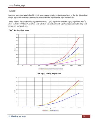
Sorting
The objective of the sorting algorithm is to rearrange the records so that their keys are ordered according to
some well-defined ordering rule.
Problem: Given an array of n real number A[1.. n].
Objective: Sort the elements of A in ascending order of their values.
Internal Sort
If the file to be sorted will fit into memory or equivalently if it will fit into an array, then the sorting method
is called internal. In this method, any record can be accessed easily.
External Sort
Sorting files from tape or disk.
In this method, an external sort algorithm must access records sequentially, or at least in the block.
Memory Requirement
1. Sort in place and use no extra memory except perhaps for a small stack or table.
2. Algorithm that use a linked-list representation and so use N extra words of memory for list pointers.
3. Algorithms that need enough extra memory space to hold another copy of the array to be sorted.](https://image.slidesharecdn.com/adanotes-180923121213/85/Analysis-and-Design-of-Algorithms-notes-22-320.jpg)
![Introduction ADA
K. Adisesha, BE M.Sc, M Tech 25
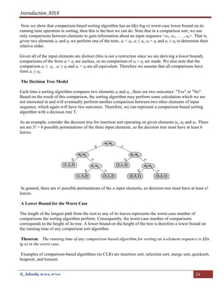
Proof Consider a decision tree of height h that sorts n elements. Since there are n! permutation of n
elements and the tree must have at least n! leaves. We have
n! ≤ 2h
Taking logarithms on both sides
(lg(n!) ≤ h
h ≥ lg(n!)
Since the lg function is monotonically increasing, from Stirling's approximation we have
n! > (n/e)n
where e = 2.71828 . . .
h ≥ (n/e)n
which is Ω(n lg n)
Bubble Sort
Bubble Sort is an elementary sorting algorithm. It works by repeatedly exchanging adjacent elements, if
necessary. When no exchanges are required, the file is sorted.
SEQUENTIAL BUBBLESORT (A)
for i ← 1 to length [A] do
for j ← length [A] downto i +1 do
If A[A] < A[j-1] then
Exchange A[j] ↔ A[j-1]
Here the number of comparison made
1 + 2 + 3 + . . . + (n - 1) = n(n - 1)/2 = O(n2
)](https://image.slidesharecdn.com/adanotes-180923121213/85/Analysis-and-Design-of-Algorithms-notes-25-320.jpg)
![Introduction ADA
K. Adisesha, BE M.Sc, M Tech 26
Clearly, the graph shows the n2
nature of the bubble sort.
In this algorithm the number of comparison is irrespective of data set i.e., input whether best or worst.
Memory Requirement
Clearly, bubble sort does not require extra memory.
Implementation
void bubbleSort(int numbers[], int array_size)
{
int i, j, temp;
for (i = (array_size - 1); i >= 0; i--)
{
for (j = 1; j <= i; j++)
{
if (numbers[j-1] > numbers[j])
{
temp = numbers[j-1];
numbers[j-1] = numbers[j];
numbers[j] = temp;
}
}
}
}
Algorithm for Parallel Bubble Sort
PARALLEL BUBBLE SORT (A)
1. For k = 0 to n-2
2. If k is even then
3. for i = 0 to (n/2)-1 do in parallel
4. If A[2i] > A[2i+1] then
5. Exchange A[2i] ↔ A[2i+1]
6. Else
7. for i = 0 to (n/2)-2 do in parallel
8. If A[2i+1] > A[2i+2] then
9. Exchange A[2i+1] ↔ A[2i+2]
10. Next k
Parallel Analysis
Steps 1-10 is a one big loop that is represented n -1 times. Therefore, the parallel time complexity is O(n). If
the algorithm, odd-numbered steps need (n/2) - 2 processors and even-numbered steps require (n/2) - 1
processors. Therefore, this needs O(n) processors.](https://image.slidesharecdn.com/adanotes-180923121213/85/Analysis-and-Design-of-Algorithms-notes-26-320.jpg)
![Introduction ADA
K. Adisesha, BE M.Sc, M Tech 27
Links
Bubble Sort
Bubble Sort (Ordinary)
Bubble Sort (Ordinary, with User Input)
Bubble Sort (More Efficient)
Bubble Sort (More Efficient, with User Input)
Simple Sort
Simple Sort (with User Input)
Insertion Sort
If the first few objects are already sorted, an unsorted object can be inserted in the sorted set in proper place.
This is called insertion sort. An algorithm consider the elements one at a time, inserting each in its suitable
place among those already considered (keeping them sorted).
Insertion sort is an example of an incremental algorithm; it builds the sorted sequence one number at a time.
INSERTION_SORT (A)
1. For j = 2 to length [A] do
2. key = A[j]
3. {Put A[j] into the sorted sequence A[1 . . j-1]
4. i ← j -1
5. while i > 0 and A[i] > key do
6. A[i+1] = A[i]
7. i = i-1
8. A[i+1] = key
Analysis
Best-Case
The while-loop in line 5 executed only once for each j. This happens if given array A is already sorted.
T(n) = an + b = O(n)
It is a linear function of n.
Worst-Case
The worst-case occurs, when line 5 executed j times for each j. This can happens if array A starts out in
reverse order
T(n) = an2
+ bc + c = O(n2
)](https://image.slidesharecdn.com/adanotes-180923121213/85/Analysis-and-Design-of-Algorithms-notes-27-320.jpg)
![Introduction ADA
K. Adisesha, BE M.Sc, M Tech 28
It is a quadratic function of n.
The graph shows the n2
complexity of the insertion sort.
Stability
Since multiple keys with the same value are placed in the sorted array in the same order that they appear in
the input array, Insertion sort is stable.
Extra Memory
This algorithm does not require extra memory.
For Insertion sort we say the worst-case running time is θ(n2
), and the best-case running time is θ(n).
Insertion sort use no extra memory it sort in place.
The time of Insertion sort is depends on the original order of a input. It takes a time in Ω(n2
) in the
worst-case, despite the fact that a time in order of n is sufficient to solve large instances in which the
items are already sorted.
Implementation
void insertionSort(int numbers[], int array_size)
{
int i, j, index;
for (i=1; i < array_size; i++)
{
index = numbers[i];
j = i;
while ((j > 0) && (numbers[j-1] > index))](https://image.slidesharecdn.com/adanotes-180923121213/85/Analysis-and-Design-of-Algorithms-notes-28-320.jpg)
![Introduction ADA
K. Adisesha, BE M.Sc, M Tech 29
{
numbers[j] = numbers[j-1];
j = j - 1;
}
numbers[j] = index;
}
}
Selection Sort
This type of sorting is called "Selection Sort" because it works by repeatedly element. It works as follows:
first find the smallest in the array and exchange it with the element in the first position, then find the second
smallest element and exchange it with the element in the second position, and continue in this way until the
entire array is sorted.
SELECTION_SORT (A)
for i ← 1 to n-1 do
min j ← i;
min x ← A[i]
for j ← i + 1 to n do
If A[j] < min x then
min j ← j
min x ← A[j]
A[min j] ← A [i]
A[i] ← min x
Selection sort is among the simplest of sorting techniques and it work very well for small files.
Furthermore, despite its evident "naïve approach "Selection sort has a quite important application because
each item is actually moved at most once, Section sort is a method of choice for sorting files with very large
objects (records) and small keys.](https://image.slidesharecdn.com/adanotes-180923121213/85/Analysis-and-Design-of-Algorithms-notes-29-320.jpg)
![Introduction ADA
K. Adisesha, BE M.Sc, M Tech 30
The worst case occurs if the array is already sorted in descending order. Nonetheless, the time require by
selection sort algorithm is not very sensitive to the original order of the array to be sorted: the test "if A[j] <
min x" is executed exactly the same number of times in every case. The variation in time is only due to the
number of times the "then" part (i.e., min j ← j; min x ← A[j] of this test are executed.
The Selection sort spends most of its time trying to find the minimum element in the "unsorted" part of the
array. It clearly shows the similarity between Selection sort and Bubble sort. Bubble sort "selects" the
maximum remaining elements at each stage, but wastes some effort imparting some order to "unsorted" part
of the array. Selection sort is quadratic in both the worst and the average case, and requires no extra
memory.
For each i from 1 to n - 1, there is one exchange and n - i comparisons, so there is a total of n -1 exchanges
and (n -1) + (n -2) + . . . + 2 + 1 = n(n -1)/2 comparisons. These observations hold no matter what the input
data is. In the worst case, this could be quadratic, but in the average case, this quantity is O(n log n). It
implies that the running time of Selection sort is quite insensitive to the input.
Implementation
void selectionSort(int numbers[], int array_size)
{
int i, j;
int min, temp;
for (i = 0; i < array_size-1; i++)
{
min = i;
for (j = i+1; j < array_size; j++)
{
if (numbers[j] < numbers[min])
min = j;](https://image.slidesharecdn.com/adanotes-180923121213/85/Analysis-and-Design-of-Algorithms-notes-30-320.jpg)
![Introduction ADA
K. Adisesha, BE M.Sc, M Tech 31
}
temp = numbers[i];
numbers[i] = numbers[min];
numbers[min] = temp;
}
}
Shell Sort
This algorithm is a simple extension of Insertion sort. Its speed comes from the fact that it exchanges
elements that are far apart (the insertion sort exchanges only adjacent elements).
The idea of the Shell sort is to rearrange the file to give it the property that taking every hth
element (starting
anywhere) yields a sorted file. Such a file is said to be h-sorted.
SHELL_SORT (A)
for h = 1 to h N/9 do
for (; h > 0; h != 3) do
for i = h +1 to i n do
v = A[i]
j = i
while (j > h AND A[j - h] > v
A[i] = A[j - h]
j = j - h
A[j] = v
i = i + 1
The function form of the running time for all Shell sort depends on the increment sequence and is unknown.
For the above algorithm, two conjectures are n(logn)2
and n1.25
. Furthermore, the running time is not
sensitive to the initial ordering of the given sequence, unlike Insertion sort.](https://image.slidesharecdn.com/adanotes-180923121213/85/Analysis-and-Design-of-Algorithms-notes-31-320.jpg)
![Introduction ADA
K. Adisesha, BE M.Sc, M Tech 32
Shell sort is the method of choice for many sorting application because it has acceptable running time even
for moderately large files and requires only small amount of code that is easy to get working. Having said
that, it is worthwhile to replace Shell sort with a sophisticated sort in given sorting problem.
Implementation
void shellSort(int numbers[], int array_size)
{
int i, j, increment, temp;
increment = 3;
while (increment > 0)
{
for (i=0; i < array_size; i++)
{
j = i;
temp = numbers[i];
while ((j >= increment) && (numbers[j-increment] > temp))
{
numbers[j] = numbers[j - increment];
j = j - increment;
}
numbers[j] = temp;
}
if (increment/2 != 0)
increment = increment/2;
else if (increment == 1)
increment = 0;](https://image.slidesharecdn.com/adanotes-180923121213/85/Analysis-and-Design-of-Algorithms-notes-32-320.jpg)
![Introduction ADA
K. Adisesha, BE M.Sc, M Tech 33
else
increment = 1;
}
}
Heap Sort
The binary heap data structures is an array that can be viewed as a complete binary tree. Each node of the
binary tree corresponds to an element of the array. The array is completely filled on all levels except
possibly lowest.
We represent heaps in level order, going from left to right. The array corresponding to the heap above is
[25, 13, 17, 5, 8, 3].
The root of the tree A[1] and given index i of a node, the indices of its parent, left child and right child can
be computed
PARENT (i)
return floor(i
LEFT (i)
return 2i
RIGHT (i)
return 2i + 1
Let's try these out on a heap to make sure we believe they are correct. Take this heap,
which is represented by the array [20, 14, 17, 8, 6, 9, 4, 1].](https://image.slidesharecdn.com/adanotes-180923121213/85/Analysis-and-Design-of-Algorithms-notes-33-320.jpg)
![Introduction ADA
K. Adisesha, BE M.Sc, M Tech 34
We'll go from the 20 to the 6 first. The index of the 20 is 1. To find the index of the left child, we calculate 1
* 2 = 2. This takes us (correctly) to the 14. Now, we go right, so we calculate 2 * 2 + 1 = 5. This takes us
(again, correctly) to the 6.
Now let's try going from the 4 to the 20. 4's index is 7. We want to go to the parent, so we calculate 7 / 2 =
3, which takes us to the 17. Now, to get 17's parent, we calculate 3 / 2 = 1, which takes us to the 20.
Heap Property
In a heap, for every node i other than the root, the value of a node is greater than or equal (at most) to the
value of its parent.
A[PARENT (i i]
Thus, the largest element in a heap is stored at the root.
Following is an example of Heap:
By the definition of a heap, all the tree levels are completely filled except possibly for the lowest level,
which is filled from the left up to a point. Clearly a heap of height h has the minimum number of elements
when it has just one node at the lowest level. The levels above the lowest level form a complete binary tree
of height h -1 and 2h
-1 nodes. Hence the minimum number of nodes possible in a heap of height h is 2h
.
Clearly a heap of height h, has the maximum number of elements when its lowest level is completely filled.
In this case the heap is a complete binary tree of height h and hence has 2h+1
-1 nodes.
Following is not a heap, because it only has the heap property - it is not a complete binary tree. Recall that
to be complete, a binary tree has to fill up all of its levels with the possible exception of the last one, which
must be filled in from the left side.](https://image.slidesharecdn.com/adanotes-180923121213/85/Analysis-and-Design-of-Algorithms-notes-34-320.jpg)
![Introduction ADA
K. Adisesha, BE M.Sc, M Tech 35
Height of a node
We define the height of a node in a tree to be a number of edges on the longest simple downward path from
a node to a leaf.
Height of a tree
The number of edges on a simple downward path from a root to a leaf. Note that the height of a tree with n
node is lg n which is (lgn). This implies that an n-element heap has height lg n
In order to show this let the height of the n-element heap be h. From the bounds obtained on maximum and
minimum number of elements in a heap, we get
2h
≤ n ≤ 2h+1
-1
Where n is the number of elements in a heap.
2h
≤ n ≤ 2h+1
Taking logarithms to the base 2
h ≤ lgn ≤ h +1
It follows that h = lgn
We known from above that largest element resides in root, A[1]. The natural question to ask is where in a
heap might the smallest element resides? Consider any path from root of the tree to a leaf. Because of the
heap property, as we follow that path, the elements are either decreasing or staying the same. If it happens to
be the case that all elements in the heap are distinct, then the above implies that the smallest is in a leaf of
the tree. It could also be that an entire subtree of the heap is the smallest element or indeed that there is only
one element in the heap, which in the smallest element, so the smallest element is everywhere. Note that
anything below the smallest element must equal the smallest element, so in general, only entire subtrees of
the heap can contain the smallest element.
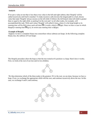
Inserting Element in the Heap](https://image.slidesharecdn.com/adanotes-180923121213/85/Analysis-and-Design-of-Algorithms-notes-35-320.jpg)
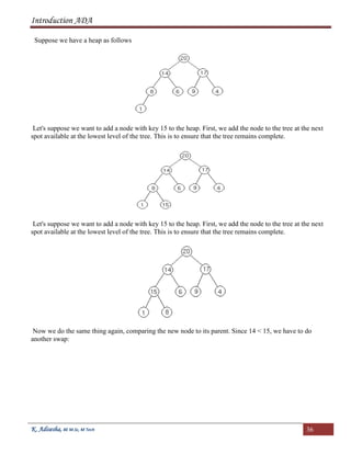
![Introduction ADA
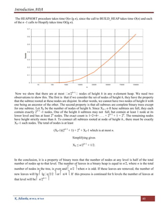
K. Adisesha, BE M.Sc, M Tech 37
Now we are done, because 15 20.
Four basic procedures on heap are
1. Heapify, which runs in O(lg n) time.
2. Build-Heap, which runs in linear time.
3. Heap Sort, which runs in O(n lg n) time.
4. Extract-Max, which runs in O(lg n) time.
Maintaining the Heap Property
Heapify is a procedure for manipulating heap data structures. It is given an array A and index i into the
array. The subtree rooted at the children of A[i] are heap but node A[i] itself may possibly violate the heap
property i.e., A[i] < A[2i] or A[i] < A[2i +1]. The procedure 'Heapify' manipulates the tree rooted at A[i] so
it becomes a heap. In other words, 'Heapify' is let the value at A[i] "float down" in a heap so that subtree
rooted at index i becomes a heap.
Outline of Procedure Heapify
Heapify picks the largest child key and compare it to the parent key. If parent key is larger than heapify
quits, otherwise it swaps the parent key with the largest child key. So that the parent is now becomes larger
than its children.
It is important to note that swap may destroy the heap property of the subtree rooted at the largest child
node. If this is the case, Heapify calls itself again using largest child node as the new root.
Heapify (A, i)
1. l ← left [i]
2. r ← right [i]
3. if l ≤ heap-size [A] and A[l] > A[i]
4. then largest ← l
5. else largest ← i
6. if r ≤ heap-size [A] and A[i] > A[largest]
7. then largest ← r
8. if largest ≠ i
9. then exchange A[i] ↔ A[largest]
10. Heapify (A, largest)](https://image.slidesharecdn.com/adanotes-180923121213/85/Analysis-and-Design-of-Algorithms-notes-37-320.jpg)
![Introduction ADA
K. Adisesha, BE M.Sc, M Tech 39
Now, 7 is greater than 6, so we exchange them.
We are at the bottom of the tree, and can't continue, so we terminate.
Building a Heap
We can use the procedure 'Heapify' in a bottom-up fashion to convert an array A[1 . . n] into a heap. Since
the elements in the subarray A[ n/2 n] are all leaves, the procedure BUILD_HEAP goes through
the remaining nodes of the tree and runs 'Heapify' on each one. The bottom-up order of processing node
guarantees that the subtree rooted at children are heap before 'Heapify' is run at their parent.
BUILD_HEAP (A)
1. heap-size (A) ← length [A]
2. For i ← floor(length[A
3. Heapify (A, i)
We can build a heap from an unordered array in linear time.
Heap Sort Algorithm
The heap sort combines the best of both merge sort and insertion sort. Like merge sort, the worst case time
of heap sort is O(n log n) and like insertion sort, heap sort sorts in-place. The heap sort algorithm starts by
using procedure BUILD-HEAP to build a heap on the input array A[1 . . n]. Since the maximum element of
the array stored at the root A[1], it can be put into its correct final position by exchanging it with A[n] (the
last element in A). If we now discard node n from the heap than the remaining elements can be made into
heap. Note that the new element at the root may violate the heap property. All that is needed to restore the
heap property.
HEAPSORT (A)
1. BUILD_HEAP (A)
2. for i ← length (A) down to 2 do
exchange A[1] ↔ A[i]
heap-size [A] ← heap-size [A] - 1
Heapify (A, 1)](https://image.slidesharecdn.com/adanotes-180923121213/85/Analysis-and-Design-of-Algorithms-notes-39-320.jpg)
![Introduction ADA
K. Adisesha, BE M.Sc, M Tech 41
Implementation
void heapSort(int numbers[], int array_size)
{
int i, temp;
for (i = (array_size / 2)-1; i >= 0; i--)
siftDown(numbers, i, array_size);
for (i = array_size-1; i >= 1; i--)
{
temp = numbers[0];
numbers[0] = numbers[i];
numbers[i] = temp;
siftDown(numbers, 0, i-1);
}
}
void siftDown(int numbers[], int root, int bottom)
{
int done, maxChild, temp;
done = 0;
while ((root*2 <= bottom) && (!done))
{
if (root*2 == bottom)
maxChild = root * 2;
else if (numbers[root * 2] > numbers[root * 2 + 1])
maxChild = root * 2;
else
maxChild = root * 2 + 1;
if (numbers[root] < numbers[maxChild])
{
temp = numbers[root];
numbers[root] = numbers[maxChild];
numbers[maxChild] = temp;
root = maxChild;
}
else
done = 1;
}
}](https://image.slidesharecdn.com/adanotes-180923121213/85/Analysis-and-Design-of-Algorithms-notes-41-320.jpg)
![Introduction ADA
K. Adisesha, BE M.Sc, M Tech 42
Merge Sort
Merge-sort is based on the divide-and-conquer paradigm. The Merge-sort algorithm can be described in
general terms as consisting of the following three steps:
1. Divide Step
If given array A has zero or one element, return S; it is already sorted. Otherwise, divide A into two
arrays, A1 and A2, each containing about half of the elements of A.
2. Recursion Step
Recursively sort array A1 and A2.
3. Conquer Step
Combine the elements back in A by merging the sorted arrays A1 and A2 into a sorted sequence.
We can visualize Merge-sort by means of binary tree where each node of the tree represents a recursive call
and each external nodes represent individual elements of given array A. Such a tree is called Merge-sort
tree. The heart of the Merge-sort algorithm is conquer step, which merge two sorted sequences into a single
sorted sequence.
To begin, suppose that we have two sorted arrays A1[1], A1[2], . . , A1[M] and A2[1], A2[2], . . . , A2[N]. The
following is a direct algorithm of the obvious strategy of successively choosing the smallest remaining
elements from A1 to A2 and putting it in A.](https://image.slidesharecdn.com/adanotes-180923121213/85/Analysis-and-Design-of-Algorithms-notes-42-320.jpg)
![Introduction ADA
K. Adisesha, BE M.Sc, M Tech 43
MERGE (A1, A2, A)
i.← j 1
A1[m+1], A2[n+1] ← INT_MAX
For k ←1 to m + n do
if A1[i] < A2[j]
then A[k] ← A1[i]
i ← i +1
else
A[k] ← A2[j]
j ← j + 1
Merge Sort Algorithm
MERGE_SORT (A)
A1[1 . . n/2 ] ← A[1 . . n/2 ]
A2[1 . . n/2 ] ← A[1 + n/2 . . n]
Merge Sort (A1)
Merge Sort (A1)
Merge Sort (A1, A2, A)
Analysis
Let T(n) be the time taken by this algorithm to sort an array of n elements dividing A into subarrays A1 and
A2 takes linear time. It is easy to see that the Merge (A1, A2, A) also takes the linear time. Consequently,
T(n) = T( n/2 ) + T( n/2 ) + θ(n)
for simplicity
T(n) = 2T (n/2) + θ(n)
The total running time of Merge sort algorithm is O(n lg n), which is asymptotically optimal like Heap sort,
Merge sort has a guaranteed n lg n running time. Merge sort required (n) extra space. Merge is not in-
place algorithm. The only known ways to merge in-place (without any extra space) are too complex to be
reduced to practical program.](https://image.slidesharecdn.com/adanotes-180923121213/85/Analysis-and-Design-of-Algorithms-notes-43-320.jpg)
![Introduction ADA
K. Adisesha, BE M.Sc, M Tech 44
Implementation
void mergeSort(int numbers[], int temp[], int array_size)
{
m_sort(numbers, temp, 0, array_size - 1);
}
void m_sort(int numbers[], int temp[], int left, int right)
{
int mid;
if (right > left)
{
mid = (right + left) / 2;
m_sort(numbers, temp, left, mid);
m_sort(numbers, temp, mid+1, right);](https://image.slidesharecdn.com/adanotes-180923121213/85/Analysis-and-Design-of-Algorithms-notes-44-320.jpg)
![Introduction ADA
K. Adisesha, BE M.Sc, M Tech 45
merge(numbers, temp, left, mid+1, right);
}
}
void merge(int numbers[], int temp[], int left, int mid, int right)
{
int i, left_end, num_elements, tmp_pos;
left_end = mid - 1;
tmp_pos = left;
num_elements = right - left + 1;
while ((left <= left_end) && (mid <= right))
{
if (numbers[left] <= numbers[mid])
{
temp[tmp_pos] = numbers[left];
tmp_pos = tmp_pos + 1;
left = left +1;
}
else
{
temp[tmp_pos] = numbers[mid];
tmp_pos = tmp_pos + 1;](https://image.slidesharecdn.com/adanotes-180923121213/85/Analysis-and-Design-of-Algorithms-notes-45-320.jpg)
![Introduction ADA
K. Adisesha, BE M.Sc, M Tech 46
mid = mid + 1;
}
}
while (left <= left_end)
{
temp[tmp_pos] = numbers[left];
left = left + 1;
tmp_pos = tmp_pos + 1;
}
while (mid <= right)
{
temp[tmp_pos] = numbers[mid];
mid = mid + 1;
tmp_pos = tmp_pos + 1;
}
for (i=0; i <= num_elements; i++)
{
numbers[right] = temp[right];
right = right - 1;
}
}](https://image.slidesharecdn.com/adanotes-180923121213/85/Analysis-and-Design-of-Algorithms-notes-46-320.jpg)

This document provides an introduction to algorithms and their analysis. It defines what an algorithm is and discusses different aspects of analyzing algorithm performance, including time complexity, space complexity, asymptotic analysis using Big O, Big Theta, and Big Omega notations. It also covers greedy algorithms, their characteristics, and examples like the knapsack problem. Greedy algorithms make locally optimal choices at each step without reconsidering prior decisions. Not all problems can be solved greedily, and the document discusses when greedy algorithms can and cannot be applied.