2. where Psat
i is the vapor pressure of component I, and P is the system
total pressure. A number of correlations for VER have been de-
veloped for hydrocarbon systems that form relatively ideal solu-
tions, but for most chemical systems, Eq. (13.4) must be corrected.
At lower pressures (below about 5 atm), the correction factor is a
liquid phase activity coefficient gL
i (sometimes called a ‘‘Raoult’s
law correction factor’’).
A more rigorous expression is derived by noting that at equi-
librium, partial fugacities of each component are the same in each
phase, that is
f v
i ¼ f L
i (13:5)
or, in terms of fugacity and activity coefficients,
yifv
i P ¼ gL
i xifL
i Psat
i (13:6)
and the VER becomes
Ki ¼
yi
xi
¼
gL
i fsat
i Psat
i
fv
i P
(13:7)
Additionally, small corrections for pressure, called Poynting
factors, belong in Eq. (13.6) but are omitted here. The new terms
are:
fsat
i ¼ fugacity coefficient of the pure component at its vapor
pressure,
fv
i ¼ partial fugacity coefficient in the vapor phase.
Equations for fugacity coefficients are derived from equations
of state or are approximated from activity coefficient charts as
functions of reduced temperature and pressure. Table 13.1 includes
them for the popular Soave equation of state. At pressures below
5–6 atm, the ratio of activity coefficients in Eq. (13.7) often is near
unity. Then the VER becomes
Ki ¼ gL
i Psat
i =P (13:8)
which is independent of the nature of the vapor phase.
Values of the activity coefficients are deduced from experi-
mental data of vapor-liquid equilibria and correlated or extended
by any one of several available equations. Values also be calculated
approximately from structural group contributions by methods
called UNIFAC and ASOG. For more than two components, the
correlating equations favored nowadays are the Wilson, the
NRTL, and UNIQUAC, and for some applications a solubility
parameter method. The first and last of these are given in Table
13.2. Calculations from measured equilibrium compositions are
made with the rearranged equation
gi ¼
fu
i P
fsat
i Psat
i
yi
xi
(13:9)
’
P
Psat
i
yi
xi
: (13:10)
The last approximation usually may be made at pressures below
5–6 atm. Then the activity coefficient is determined by the vapor
pressure, the system pressure, and the measured equilibrium com-
positions.
Since the fugacity and activity coefficients are mathematically
complex functions of the compositions, finding corresponding
compositions of the two phases at equilibrium when the equations
are known requires solutions by trial. Suitable procedures for
making flash calculations are presented in the next section, and in
TABLE 13.1. The Soave Equation of State and Fugacity
Coefficients
Equation of State
P ¼
RT
V b
aa
V(V þ b)
z3
z2
þ (A B B2
)z AB ¼ 0
Parameters
a ¼ 0:42747R2
T2
c =Pc0
b ¼ 0:08664RTc =Pc
a ¼ [1 þ (0:48508 þ 1:55171! 0:15613!2
)(1 T0:5
r )]2
a ¼ 1:202 exp ( 0:30288Tr ) and for hydrogen
(Graboski and Daubert, 1979)
A ¼ aaP=R2
T2
¼ 0:42747aPr =T2
r
B ¼ bP=RT ¼ 0:08664Pr =Tr
Mixtures
aa ¼ SSyi yj (aa)ij
b ¼ Syi bi
A ¼ SSyi yj Aij
B ¼ Syi Bi
Cross parameters
(aa)ij ¼ (1 kij )
ffiffiffiffiffiffiffiffiffiffiffiffiffiffiffiffiffiffiffiffi
(aa)i (aa)j
p
kij in table
kij ¼ 0 for hydrocarbon pairs and hydrogen
Correlations in Terms of Absolute Differences between
Solubility Parameters of the Hydrocarbon, dHC and of the Inorganic
Gas
Gas kij
H2S 0:0178 þ 0:0244jdHC 8:80j
CO2 0:1294 0:0292jdHC 7:12j2
0:0222jdHC 7:12j2
N2 0:0836 þ 0:1055jdHC 4:44j 0:0100jdHC 4:44j2
Fugacity Coefficient of a Pure Substance
Inf¼ z 1 In z 1
b
V
aa
bRT
In 1 þ
b
V
¼ z 1 In(z B)
A
B
In 1 þ
B
z
Fugacity Coefficients in Mixtures
Infi¼
bi
b
(z 1) In z 1
b
V
þ
aa
bRT
bi
b
2
a
X
j
yj (aa)ij
#
In 1 þ
b
V
¼
Bi
B
(z 1) ¼ In(z B) þ
A
B
Bi
B
2
aa
X
j
yj (aa)ij
#
In 1 þ
B
2
(Walas, 1985).
396 DISTILLATION AND GAS ABSORPTION
3. greater detail in some books on thermodynamics, for instance, the
one by Walas (1985). In making such calculations, it is usual to start
by assuming ideal behavior, that is,
^
fu
i =fsat
i ¼ gi ¼ 1: (13:11)
After the ideal equilibrium compositions have been found, they are
used to find improved values of the fugacity and activity coeffi-
cients. The process is continued to convergence.
RELATIVE VOLATILITY
The compositions of vapor and liquid phases of a binary system at
equilibrium sometimes can be related by a constant relative volatil-
ity which is defined as
a12 ¼
y1
x1
=
y2
x2
¼
y1
1 y1
=
x1
1 x1
: (13:12)
Then
y1
1 y1
¼ a12
x1
1 x1
: (13:13)
In terms of vaporization equilibrium ratios,
a12 ¼ K1=K2 ¼ gL
1 Psat
1 =g2Psat
2 , (13:14)
and when Raoult’s law applies (gL
¼ 1:0) the relative volatility is
the ideal value,
aideal ¼ Psat
1 =Psat
2 : (13:15)
Usually the relative volatility is not truly constant but is found to
depend on the composition, for example,
a12 ¼ k1 þ k2x1: (13:16)
Other relations that have been proposed are
y1
1 y1
¼ k1 þ k2
x1
1 x1
(13:17)
and
y1
1 y1
¼ k1
x1
1 x1
k2
: (13:18)
A variety of such relations is discussed by Hala (Vapor–Liquid
Equilibria, Pergamon London, 1967). Other expressions can be
deduced from Eq. (13.14) and some of the equations for activity
coefficients, for instance, the Scatchard-Hildebrand of Table 13.2.
Then
a12 ¼
y1
x1
=
y2
x2
¼
Psat
1
Psat
2
exp
(d1 d2)2
RT
[V1(1 f1)2
V2f2
1]
( )
,
(13:19)
where
f1 ¼
V1x1
V1x1 þ V2x2
(13:20)
is the volume fraction of component 1 in the mixture.
Beyond a certain complexity these analytical relations between
vapor and liquid compositions lose their utility. The simplest
one, Eq. (13.13), is of value in the analysis of multistage separating
equipment. When the relative volatility varies modestly from
stage to stage, a geometric mean often is an adequate value to
use. Applications are made later. Example 13.1 examines
two ways of interpreting dependence of relative volatility on
composition.
BINARY x y DIAGRAMS
Equilibria between the components of a binary mixture are ex-
pressed as a functional relation between the mol fractions of the
usually more volatile component in the vapor and liquid phases,
y ¼ f (x): (13:21)
The definition of relative volatility, Eq (13.13) is rearranged into
this form:
y ¼
ax
1 þ (a 1)x
(13:22)
Representative x y diagrams appear in Figure 13.3; one should
note that the y and x scales are in weight percent, not the usual mole
percent. Generally they are plots of direct experimental data, but
they can be calculated from fundamental data of vapor pressure
and activity coefficients. The basis is the bubblepoint condition:
y1 þ y2 ¼
g1Psat
1
P
x1 þ
g2Psat
2
P
(1 x1) ¼ 1: (13:23)
In order to relate y1 and x1, the bubblepoint temperatures are found
over a series of values of x1. Since the activity coefficients depend on
the composition of the liquid and both activity coefficients and
vapor pressures depend on the temperature, the calculation requires
a respectable effort. Moreover, some vapor-liquid measurements
must have been made for evaluation of a correlation of activity
coefficients. The method does permit calculation of equilibria at
several pressures since activity coefficients are substantially inde-
pendent of pressure. A useful application is to determine the effect
of pressure on azeotropic composition (Walas, 1985, p. 227).
13.2. SINGLE-STAGE FLASH CALCULATIONS
The problems of interest are finding the conditions for onset of
vaporization, the bubble-point; for the onset of condensation, the
dewpoint; and the compositions and the relative amounts of vapor
and liquid phases at equilibrium under specified conditions of
temperature and pressure or enthalpy and pressure. The first
cases examined will take the Ki to be independent of composition.
These problems usually must be solved by iteration, for which the
Newton–Raphson method is suitable. The dependence of K on
temperature may be represented adequately by
Ki ¼ exp [Ai Bi=(T þ Ci)]: (13:24)
An approximate relation for the third constant is
Ci ¼ 18 0:19Tbi, (13:25)
where Tbi is the normal boiling point in 8K. The dependence of K on
pressure may be written simply as
Ki ¼ aiPbi
: (13:26)
13.2. SINGLE-STAGE FLASH CALCULATIONS 397
4. Linear expressions for the enthalpies of the two phases are
hi ¼ ai þ biT, (13:27)
Hi ¼ ci þ diT, (13:28)
assuming negligible heats of mixing. The coefficients are
evaluated from tabulations of pure component enthalpies. First
derivatives are needed for application of the Newton-Raphson
method:
@Ki=@T ¼ BiKi=(T þ Ci)2
, (13:29)
@Ki=@P ¼ biKi=P: (13:30)
BUBBLE-POINT TEMPERATURE AND PRESSURE
The temperature at which a liquid of known composition first
begins to boil is found from the equation
f (T) ¼
X
Kixi 1 ¼ 0, (13:31)
where the Ki are known functions of the temperature. In terms of
Eq. (13.24) the Newton–Raphson algorithm is
T ¼ T
1 þ
P
Kixi
P
[BiKixi=(T þ Ci)2
]
: (13:32)
Similarly, when Eq. (13.26) represents the effect of pressure, the
bubble-point pressure is found with the N-R algorithm:
f (P) ¼
X
Kixi 1 ¼ 0, (13:33)
P ¼ P
1 þ
P
aiPbi
xi
P
aibiPbi1
i xi
: (13:34)
DEWPOINT TEMPERATURE AND PRESSURE
The temperature or pressure at which a vapor of known compos-
ition first begins to condense is given by solution of the appropriate
equation,
f (T) ¼
X
yi=Ki 1 ¼ 0, (13:35)
TABLE 13.2. Activity Coefficients from Solubility Parameters and from the Wilson Equation
Binary Mixtures
Name Parameters lng1 and lng2
Scatchard–Hildebrand d1, d2
V1
RT
(1 f1)2
(d1 d2)2
V2
RT
f2
1(d1 d2)2
f1 ¼ V1x1=(V1x1 þ V2x2)
Wilson l12, l21 ln (x1 þ L12x2) þ x2
L12
x1 þ L12x2
L21
L21x1 þ x2
ln (x2 þ L21x1) x1
L12
x1 þ L12x2
L21
L21x1 þ x2
L12 ¼
VL
2
VL
1
exp l12
RT
L21 ¼
VL
1
VL
2
exp
l21
RT
VL
i molar volume of pure liquid component i.
Ternary Mixtures
ln g1 ¼ 1 ln (x1Li1 þ x2Li2 þ x3Li3)
x1L1i
x1 þ x2L12 þ x3L13
x2L2i
x1L21 þ x2 þ x3L23
x3L3i
x1L31 þ x2L32 þ x3
Lii ¼ 1
Multicomponent Mixtures
Equation Parameters lngi
Scatchard–Hildebrand di Vi
RT
di
X
j
xj Vj dj
P
k xk Vk
#2
Wilson Lij ¼
VL
j
VL
i
exp
lij
RT
ln
X
m
j¼1
xj Lij
!
þ 1
X
m
k¼1
xk Lki
P
m
j¼1
xj Lkj
Lij ¼ Ljj ¼ 1
398 DISTILLATION AND GAS ABSORPTION
5. f (P) ¼
X
yi=Ki 1 ¼ 0: (13:36)
In terms of Eqs. (13.24) and (13.26) the N–R algorithms are
T ¼ T þ
1 þ
P
yi=Ki
P
[(yi=K2
i )@Ki=@T]
¼ T þ
1 þ
P
yi=Ki
P
[Biyi=Ki(T þ Ci)2
]
,
(13:37)
P ¼ P þ
1 þ
P
yi=Ki
P
[(yi=K2
i )@Ki=@P]
¼ P þ
( 1 þ
P
yi=Ki)P
P
(biyi=Ki)
:
(13:38)
FLASH AT FIXED TEMPERATURE AND PRESSURE
At temperatures and pressures between those of the bubblepoint
and dewpoint, a mixture of two phases exists whose amounts and
compositions depend on the conditions that are imposed on the
system. The most common sets of such conditions are fixed T and
P, or fixed H and P, or fixed S and P. Fixed T and P will be
considered first.
For each component the material balances and equilibria are:
Fzi ¼ Lxi þ Vyi, (13:39)
yi ¼ Kixi: (13:40)
On combining these equations and introducing b ¼ V=F, the frac-
tion vaporized, the flash condition becomes
f (b) ¼ 1 þ
X
xi ¼ 1 þ
X zi
1 þ b(Ki 1)
¼ 0, (13:41)
and the corresponding N–R algorithm is
b ¼ b þ
1 þ
P
[zi=(1 þ b(Ki 1))]
P
{(Ki 1)zi=[1 þ b(Ki 1)]2
}
: (13:42)
After b has been found by successive approximation, the phase
compositions are obtained with
xi ¼
zi
1 þ b(Ki 1)
, (13:43)
yi ¼ Kixi: (13:44)
A starting value of b ¼ 1 always leads to a converged solution by
this method.
FLASH AT FIXED ENTHALPY AND PRESSURE
The problem will be formulated for a specified final pressure
and enthalpy, and under the assumption that the enthalpies are
additive (that is, with zero enthalpy of mixing) and are known
functions of temperature at the given pressure. The enthalpy bal-
ance is
HF ¼ (1 b)
X
xiHiL þ b
X
yiHiV (13:45)
EXAMPLE 13.1
Correlation of Relative Volatility
Data for the system ethanol þ butanol at 1 atm are taken from the
collection of Kogan (1966, #1038). The values of
x=(100 x), y=(100 y), and a are calculated and plotted. The
plot on linear coordinates shows that relative volatility does not
plot linearly with x, but from the linear log–log plot it appears that
y
100 y
¼ 4:364
x
100 x
1:045
or a ¼ 4:364
x
100 x
0:045
:
x y x y
0 0 39.9 74.95
3.45 12.5 53.65 84.3
6.85 22.85 61.6 88.3
10.55 32.7 70.3 91.69
14.5 41.6 79.95 95.08
18.3 49.6 90.8 97.98
28.4 63.45 100.0 100.0
x a x=100 x y=100 y
3.5 4.00 0.04 0.14
6.9 4.03 0.07 0.30
10.6 4.12 0.12 0.49
14.5 4.20 0.17 0.71
18.8 4.25 0.23 0.98
26.4 4.38 0.40 1.74
39.9 4.51 0.66 2.99
53.7 4.64 1.16 5.37
61.6 4.70 1.60 7.55
70.3 4.66 2.37 11.03
80.0 4.85 3.99 19.33
90.8 4.91 9.87 48.50
13.2. SINGLE-STAGE FLASH CALCULATIONS 399
6. ¼ (1 b)
X ziHiL
1 þ b(Ki 1)
þ b
X KiziHiV
1 þ b(Ki 1)
: (13:46)
This equation and the flash Eq. (13.41) constitute a set:
f (b,T) ¼ 1 þ
X zi
1 þ b(Ki 1)
¼ 0, (13:47)
g(b, T) ¼ HF (1 b)
X ziHiL
1 þ b(Ki 1)
b
X KiziHiV
1 þ b(Ki 1)
¼ 0,
(13:48)
from which the phase split b and temperature can be found when
the enthalpies and the vaporization equilibrium ratios are known
functions of temperature. The N–R method applied to Eqs. (13.47
and 13.48) finds corrections to initial estimates of b and T by
solving the linear equations
h
@f
@b
þ k
@f
@T
þ f ¼ 0, (13:49)
h
@g
@b
þ k
@g
@T
þ g ¼ 0, (13:50)
where all terms are evaluated at the assumed values (b0, T0) of the
two unknows. The corrected values, suitable for the next trial if that
is necessary, are
b ¼ b0 þ h, (13:51)
T ¼ T0 þ K: (13:52)
Example 13.2 applies these equations for dewpoint, bubblepoint,
and flashes.
EQUILIBRIA WITH Ks DEPENDENT ON COMPOSITION
The procedure will be described only for the case of bubblepoint
temperature for which the calculation sequence is represented on
Figure 13.4. Equations 13.7 and 13.31 are combined as
f (T) ¼
X gifsat
i Psat
i
^
fiP
xi 1 ¼ 0: (13:53)
Figure 13.3. Some vapor-liquid composition diagrams at essentially atmospheric pressure. This is one of four such diagrams in the original
reference (Kirschbaum, 1969). Compositions are in weight fractions of the first-named.
400 DISTILLATION AND GAS ABSORPTION
7. The liquid composition is known for a bubble-point determination,
but the temperature is not at the start, so that starting estimates
must be made for both activity and fugacity coefficients. In the flow
diagram, the starting values are proposed to be unity for all the
variables. After a trial value of the temperature is chosen, subse-
quent calculations on the diagram can be made directly. The correct
value of T has been chosen when
P
yi ¼ 1.
Since the equations for fugacity and activity coefficients are
complex, solution of this kind of problem is feasible only by com-
puter. Reference is made in Example 13.3 to such programs. There
also are given the results of such a calculation which reveals the
magnitude of deviations from ideality of a common organic system
at moderate pressure.
13.3. EVAPORATION OR SIMPLE DISTILLATION
As a mixture of substances is evaporated, the residue becomes
relatively depleted in the more volatile constituents. A relation for
EXAMPLE 13.2
Vaporization and Condensation of a Ternary Mixture
For a mixture of ethane, n-butane, and n-pentane, the bubblepoint
and dewpoint temperatures at 100 psia, a flash at 1008F and
100 psia, and an adiabatic flash at 100 psia of a mixture initially
liquid at 1008F will be determined. The overall composition zi, the
coefficients A, B, and C of Eq. (13.21) and the coefficients a, b, c,
and d of Eqs. (13.27) and (13.28) are tabulated:
The bubble-point temperature algorithm is
T ¼ T
1 þ SKixi
S[BiKixi=(T þ Ci)2
]
, (13:32)
and the dewpoint temperature algorithm is
T ¼ T þ
1 þ
P
yi=Ki
P
[Biyi=Ki(T þ Ci)2
]
: (13:33)
Results of successive iterations are
The algorithm for the fraction vapor at specified T and P is
b ¼
V
F
¼ b þ
1 þ Szi=(1 þ b(Ki 1))
S(Ki 1)zi=(1 þ b(Ki 1))2
, (13:42)
and the equations for the vapor and liquid compositions are
xi ¼ zi=(1 þ b(Ki 1)), (13:43)
yi ¼ Kixi: (13:44)
Results for successive iterations for b and the final phase compo-
sitions are
Adiabatic flash calculation: Liquid and vapor enthalpies off
charts in the API data book are fitted with linear equations
h ¼ a þ bT(
F), (13:27)
H ¼ c þ dT(
F): (13:28)
The inlet material to the flash drum is liquid at 1008F, with
H0 ¼ 8; 575:8 Btu=lb mol. The flash Eq. (13.42) applies to this part
of the example. The enthalpy balance is
H0 ¼ 8575:8
¼ (1 b)SMixihi þ bSMiyiHi
(13:45)
¼ (1 b)S
Mizihi
1 þ b(Ki 1)
þ bS
KiMiziHi
1 þ b(Ki 1)
: (13:46)
The procedure consists of the steps.
1. Assume T.
2. Find the Ki, hi, and Hi.
3. Find b from the flash equation (13.42).
4. Evaluate the enthalpy of the mixture and compare with H0,
Eq. (13.46).
The results of several trials are shown:
The final VERs and the liquid and vapor compositions are:
The numerical results were obtained with short computer programs
which are given in Walas (1985, p. 317).
Coefficients
z A B C a b c d
C2 0.3 5.7799 2167.12 30.6 122 0.73 290 0.45
nC4 0.3 6.1418 3382.90 60.8 96 0.56 267 0.34
nC5 0.4 6.4610 3978.36 73.4 90 0.55 260 0.40
Bubble-point Dewpoint
1000.0000 700.0000
695.1614 597.8363
560.1387 625.9790
506.5023 635.3072
496.1742 636.0697
495.7968 636.0743
495.7963 636.0743
b zi xi yi
1.0000 C2 0.3 0.1339 0.7231
0.8257 nC4 0.3 0.3458 0.1833
0.5964 nC5 0.4 0.5203 0.0936
0.3986
0.3038
0.2830
0.2819
T (8R) b H
530.00 0.1601 8475.70
532.00 0.1681 8585.46
531.82 0.1674 8575.58 8575.8, check.
K x y
C2 4.2897 0.1935 0.8299
nC4 0.3534 0.3364 0.1189
nC5 0.1089 0.4701 0.0512
13.3. EVAPORATION OR SIMPLE DISTILLATION 401
8. binary mixtures due to Rayleigh is developed as follows: The
differential material balance for a change dL in the amount of
liquid remaining is
ydL ¼ d(LX) ¼ Ldx þ XdL: (13:54)
Upon rearrangement and integration, the result is
ln
L
L0
¼
ðx
x0
dx
x y
: (13:55)
In terms of a constant relative volatility
y ¼
ax
1 þ (a 1)x0
(13:56)
the integral becomes
ln
L
L0
¼
1
x 1
ln
x(1 x0)
x0(1 x)
þ ln
1 x0
1 x
: (13:57)
MULTICOMPONENT MIXTURES
Simple distillation is not the same as flashing because the vapor is
removed out of contact with the liquid as soon as it forms, but the
process can be simulated by a succession of small flashes of residual
liquid, say 1% of the original amount each time. After n intervals,
the amount of residual liquid F is
F ¼ L0(1 0:01n) (13:58)
and
b ¼
V
F
¼
0:01L0
(1 0:01n)L0
¼
0:01
1 0:01n
: (13:59)
Then the flash equation (13.41) becomes a function of temperature,
f (Tn) ¼ 1 þ
X zi
1 þ 0:01(Ki 1)=(1 0:01n)
¼ 0: (13:60)
Here zi is the composition at the end of interval n and Ki also may
be taken at the temperature after interval n. The composition is
found by material balance as
Lzi ¼ L0(1 0:01n)zi ¼ L0 zi0 0:01
X
n
k¼1
yik
#
, (13:61)
where each composition yik of the flashed vapor is found from Eqs.
(13.43) and (13.44)
yi ¼ Kixi ¼
Kizi
1 þ 0:01(Ki 1)=(1 0:01n)
(13:62)
and is obtained during the process of evaluating the temperature
with Eq. (13.60). The VERs must be known as functions of tem-
perature, say with Eq. (13.24).
13.4. BINARY DISTILLATION
Key concepts of the calculation of distillation are well illustrated
by analysis of the distillation of binary mixtures. Moreover, many
real systems are essentially binary or can be treated as binaries
made up of two pseudo components, for which it is possible to
calculate upper and lower limits to the equipment size for a desired
separation.
Figure 13.4. Calculation diagram for bubblepoint temperature.
(Walas, 1985).
EXAMPLE 13.3
Bubble-Point Temperature with the Virial and Wilson Equations
A mixture of acetone (1) þ butanone (2) þ ethylacetate (3) with the
composition x1 ¼ x2 ¼ 0:3 and x3 ¼ 0:4 is at 20 atm. Data for the
system such as vapor pressures, critical properties, and Wilson
coefficients are given with a computer program in Walas (1985,
p. 325). The bubblepoint temperature was found to be 468.7 K.
Here only the properties at this temperature will be quoted to show
deviations from ideality of a common system. The ideal and real Ki
differ substantially.
Component fsat ^
fv
fsat
=^
fv
g
1 0.84363 0.84353 1.00111 1.00320
2 0.79219 0.79071 1.00186 1.35567
3 0.79152 0.78356 1.00785 1.04995
Component Kideal Kreal y
1 1.25576 1.25591 0.3779
2 0.72452 0.98405 0.2951
3 0.77266 0.81762 0.3270
402 DISTILLATION AND GAS ABSORPTION
9. The calculational base consists of equilibrium relations and
material and energy balances. Equilibrium data for many binary
systems are available as tabulations of x vs. y at constant tempera-
ture or pressure or in graphical form as on Figure 13.3. Often they
can be extended to other pressures or temperatures or expressed in
mathematical form as explained in Section 13.1. Sources of equilib-
rium data are listed in the references. Graphical calculation of
distillation problems often is the most convenient method, but
numerical procedures may be needed for highest accuracy.
MATERIAL AND ENERGY BALANCES
In terms of the nomenclature of Figure 13.5, the balances between
stage n and the top of the column are
Vnþ1ynþ1 ¼ Lnxn þ DxD, (13:63)
Vnþ1Hnþ1 ¼ Lnhn þ DhD þ Qc (13:64)
¼ Lnhn þ DQ0
, (13:65)
where
Q0
¼ hD þ Qc=D (13:66)
is the enthalpy removed at the top of the column per unit of
overhead product. These balances may be solved for the liquid/
vapor ratio as
Ln
Vnþ1
¼
ynþ1 xD
xn xD
¼
Q0
Hnþ1
Q0 hn
(13:67)
and rearranged as a combined material and energy balance as
Ln
Vnþ1
¼
ynþ1 xD
xn xD
xn þ
Hnþ1 hn
Q0 hn
xD: (13:68)
Similarly the balance between plate m below the feed and the
bottom of the column can be put in the form
ym ¼
Q00
Hm
Q00 hmþ1
xmþ1 þ
hmþ1 Hm
hmþ1 Q00
xB, (13:69)
where
Q00
¼ hB Qb=B (13:70)
is the enthalpy removed at the bottom of the column per unit of
bottoms product.
For the problem to be tractable, the enthalpies of the two
phases must be known as functions of the respective phase com-
positions. When heats of mixing and heat capacity effects are small,
the enthalpies of mixtures may be compounded of those of the pure
components; thus
H ¼ yHa þ (1 y)Hb, (13:71)
h ¼ xha þ (1 x)hb, (13:72)
where Ha and Hb are vapor enthalpies of the pure components at
their dewpoints and ha and hb are corresponding liquid enthalpies
at their bubblepoints.
Overall balances are
F ¼ D þ B, (13:73)
FzF ¼ DxD þ BxB, (13:74)
FHF ¼ DhD þ BhB: (13:75)
In the usual distillation problem, the operating pressure, the
feed composition and thermal condition, and the desired product
compositions are specified. Then the relations between the reflux
rates and the number of trays above and below the feed can be
found by solution of the material and energy balance equations
together with a vapor–liquid equilibrium relation, which may be
written in the general form
f (xn,yn) ¼ 0: (13:76)
The procedure starts with the specified terminal compositions and
applies the material and energy balances such as Eqs. (13.63) and
(13.64) and equilibrium relations alternately stage by stage. When
the compositions from the top and from the bottom agree closely,
the correct numbers of stages have been found. Such procedures
will be illustrated first with a graphical method based on constant
molal overflow.
CONSTANT MOLAL OVERFLOW
When the molal heats of vaporization of the two components are
equal and the tower is essentially isothermal throughout, the molal
Figure 13.5. Model of a fractionating tower.
13.4. BINARY DISTILLATION 403
10. flow rates Ln and Vn remain constant above the feed tray, and Lm
and Vm likewise below the feed. The material balances in the two
sections are
ynþ1 ¼
Ln
Vnþ1
xn þ
D
Vnþ1
xD, (13:63)
ym ¼
Lmþ1
Vm
xmþ1
B
Vm
xB: (13:77)
The flow rates above and below the feed stage are related by the
liquid–vapor proportions of the feed stream, or more generally by
the thermal condition of the feed, q, which is the ratio of the heat
required to convert the feed to saturated vapor and the heat of
vaporization, that is,
q ¼ (Hsat
F HF )=(DH)vap: (13:78)
For instance, for subcooled feed q 1, for saturated liquid q ¼ 1,
and for saturated vapor q ¼ 0. Upon introducing also the reflux
ratio
R ¼ Ln=D, (13:79)
the relations between the flow rates become
Lm ¼ Ln þ qF ¼ RD þ qF, (13:80)
Vm ¼ Lm B ¼ RD þ qF B: (13:81)
Accordingly, the material balances may be written
y ¼
R
R þ 1
xn þ
1
R þ 1
xD, (13:82)
ym ¼
RD þ qF
RD þ qF B
xmþ1
B
RD þ qF B
xB: (13:83)
The coordinates of the point of intersection of the material balance
lines, Eqs. (13.82) and (13.83), are located on a ‘‘q-line’’ whose
equation is
y ¼
q
q 1
x þ
1
q 1
xF : (13:84)
Figure 13.6 (b) shows these relations.
BASIC DISTILLATION PROBLEM
The basic problem of separation by distillation is to find the
numbers of stages below and above the feed stage when the quan-
tities xF , xD, xB, F, D, B, and R are known together with the
phase equilibrium relations. This means that all the terms in Eqs.
13.82 and 13.85 are to be known except the running x’s and y’s. The
problem is solved by starting with the known compositions, xD and
xB, at each end and working one stage at a time towards the feed
stage until close agreement is reached between the pairs (xn, yn) and
(xm, ym). The procedure is readily implemented on a programmable
calculator; a suitable program for the enriching section is included
in the solution of Example 13.4. A graphical solution is convenient
and rapid when the number of stages is not excessive, which
depends on the scale of the graph attempted.
Figure 13.6 illustrates various aspects of the graphical method.
A minimum number of trays is needed at total reflux, that is, with
no product takeoff. Minimum reflux corresponds to a separation
requiring an infinite number of stages, which is the case when the
equilibrium curve and the operating lines touch somewhere. Often
this can occur on the q-line, but another possibility is shown on
Figure 13.6(e). The upper operating line passes through point
(xD, xD) and xD=(R þ 1) on the left ordinate. The lower operating
line passes through the intersection of the upper with the q-line and
point (xB, xB). The feed tray is the one that crosses the intersection
of the operating lines on the q-line. The construction is shown with
Example 13.5. Constructions for cases with two feeds and with two
products above the feed plate are shown in Figure 13.7.
Optimum Reflux Ratio. The reflux ratio affects the cost of the
tower, both in the number of trays and the diameter, as well as the
cost of operation which consists of costs of heat and cooling supply
and power for the reflux pump. Accordingly, the proper basis for
choice of an optimum reflux ratio is an economic balance. The
sizing and economic factors are considered in a later section, but
reference may be made now to the results of such balances sum-
marized in Table 13.3. The general conclusion may be drawn that
the optimum reflux ratio is about 1.2 times the minimum, and also
that the number of trays is about 2.0 times the minimum. Although
these conclusions are based on studies of systems with nearly ideal
vapor-liquid equilibria near atmospheric pressure, they often are
applied more generally, sometimes as a starting basis for more
detailed analysis of reflux and tray requirements.
Azeotropic and Partially Miscible Systems. Azeotropic mix-
tures are those whose vapor and liquid equilibrium compositions
are identical. Their x–y lines cross or touch the diagonal. Partially
miscible substances form a vapor phase of constant composition
over the entire range of two-phase liquid compositions; usually the
horizontal portion of the x–y plot intersects the diagonal, but those
of a few mixtures do not, notably those of mixtures of methyl-
ethylketone and phenol with water. Separation of azeotropic mix-
tures sometimes can be effected in several towers at different
pressures, as illustrated by Example 13.6 for ethanol-water mix-
tures. Partially miscible constant boiling mixtures usually can be
separated with two towers and a condensate phase separator, as
done in Example 13.7 for n-butanol and water.
UNEQUAL MOLAL HEATS OF VAPORIZATION
Molal heats of vaporization often differ substantially, as the few
data of Table 13.4 suggest. When sensible heat effects are small,
however, the condition of constant molal overflow still can be
preserved by adjusting the molecular weight of one of the compon-
ents, thus making it a pseudocomponent with the same molal heat
of vaporization as the other substance. The x–y diagram and all of
the compositions also must be converted to the adjusted molecular
weight. Example 13.5 compares tray requirements on the basis of
true and adjusted molecular weights for the separation of ethanol
and acetic acid whose molal heats of vaporization are in the ratio
1.63. In this case, the assumption of constant molal overflow with
the true molecular weight overestimates the tray requirements.
A more satisfactory, but also more laborious, solution of the prob-
lem takes the enthalpy balance into account, as in the next section.
MATERIAL AND ENERGY BALANCE BASIS
The enthalpies of mixtures depend on their compositions as well as
the temperature. Enthalpy–concentration diagrams of binary mix-
tures, have been prepared in general form for a few important
systems. The most comprehensive collection is in Landolt-Börn-
stein [IV4b, 188, (1972)] and a few diagrams are in Perry’s Chemical
Engineers’ Handbook, for instance, of ammonia and water, of
ethanol and water, of oxygen and nitrogen, and some others.
Such diagrams are named after Merkel.
404 DISTILLATION AND GAS ABSORPTION
11. For purposes of distillation calculations, a rough diagram
of saturated vapor and liquid enthalpy concentration lines
can be drawn on the basis of pure component enthalpies.
Even with such a rough diagram, the accuracy of distillation calcu-
lation can be much superior to those neglecting enthalpy balances
entirely. Example 13.8 deals with preparing such a Merkel
diagram.
A schematic Merkel diagram and its application to distillation
calculations is shown in Figure 13.8. Equilibrium compositions of
vapor and liquid can be indicated on these diagrams by tielines, but
are more conveniently used with associated x–y diagrams as shown
with this figure. Lines passing through point P with coordinates
(xD, Q) are represented by Eq. (13.68) and those through point Q
with coordinates (xB, Q00
) by Eq. (13.69). Accordingly, any line
through P to the right of PQ intersects the vapor and liquid en-
thalpy lines in corresponding (xn, ynþ1) and similarly the intersec-
tions of random lines through Q determine corresponding
(xmþ1, ym). When these coordinates are transferred to the x–y
diagram, they determine usually curved operating lines. Figure
13.8 (b) illustrates the stepping off process for finding the number
of stages. Points P, F, and Q are collinear.
The construction for the minimum number of trays is inde-
pendent of the heat balance. The minimum reflux corresponds to a
minimum condenser load Q and hence to a minimum value of
Q0
¼ hD þ Qc=D. It can be found by trial location of point P until
an operating curve is found that touches the equilibrium curve.
ALGEBRAIC METHOD
Binary systems of course can be handled by the computer programs
devised for multicomponent mixtures that are mentioned later.
Constant molal overflow cases are handled by binary computer
programs such as the one used in Example 13.4 for the enriching
section which employ repeated alternate application of material
Figure 13.6. Features of McCabe–Thiele diagrams for constant modal overflow. (a) Operating line equations and construction and
minimum reflux construction. (b) Orientations of q-lines, with slope ¼ q=(q 1), for various thermal conditions of the feed. (c) Minimum
trays, total reflux. (d) Operating trays and reflux. (e) Minimum reflux determined by point of contact nearest xD.
13.4. BINARY DISTILLATION 405
12. EXAMPLE 13.4
Batch Distillation of Chlorinated Phenols
A mixture of chlorinated phenols can be represented as an equiva-
lent binary with 90% 2,4-dichlorphenol (DCP) and the balance
2,4,6-trichlorphenol with a relative volatility of 3.268. Product
purity is required to be 97.5% of the lighter material, and the
residue must be below 20% of 2,4-DCP. It is proposed to use a
batch distillation with 10 theoretical stages. Vaporization rate will
be maintained constant.
a. For operation at constant overhead composition, the variations
of reflux ratio and distillate yield with time will be found.
b. The constant reflux ratio will be found to meet the overhead and
bottoms specifications.
a. At constant overhead composition, yD ¼ 0:975: The compo-
sition of the residue, x10, is found at a series of reflux ratios
between the minimum andthe value that gives a residue composition
of 0.2.
With q ¼ 1 and xn ¼ 0:9,
yn ¼
axn
1 þ (a 1)xn
¼
3:268(0:9)
1 þ 2:268(0:9)
¼ 0:9671,
Rm=(Rm þ 1) ¼
0:975 0:9671
0:975 0:9
¼ 0:1051,
;Rm ¼ 0:1174:
The btms compositions at a particular value of R are found by
successive applications of the equations
xn ¼
yn
a (a 1)yn
, (1)
ynþ1 ¼
R
R þ 1
xn þ
1
R þ 1
yD: (2)
Start with y1 ¼ yD ¼ 0:975. The calculations are performed
with the given computer program and the results are tabulated.
The values of L=L0 are found by material balance:
L=L0 ¼ (0:975 0:900)=(0:975 xL) (3)
The values of V=L0 are found with Eq. 13.110
V
L0
¼ (yD xL0
)
Z xL
xL0
R þ 1
( yD xL)2
dxL
¼ (0:975 0:900)
Z xL
0:9
R þ 1
(0:975 xL)2
dxL:
(4)
From the tabulation, the cumulative vaporization is
V=L0 ¼ 1:2566:
The average reflux ratio is
R ¼
V D
D
¼
V
D
1 ¼
V
L0 L
1 ¼
V=L0
1 L=L0
1
¼
1:2566
1 0:0968
1 ¼ 0:3913:
10 ! Example 13.4. Distillation at constant Yd
20 A ¼ 3:268
30 OPTION BASE 1
40 DIM X(10), Y(12)
50 Y(1) ¼ .975
60 INPUT R
70 FOR N¼1 TO 10
80 X(N)¼1 / (A/Y(N)Aþ1)
90 Y(N þ 1) ¼ 1=(R þ 1) (R X(N) þ Y(1))
100 NEXT N
110 Z ¼ (Y(1) .9)/(Y(1)X(10) )! = L/Lo
120 I ¼ (R þ 1)=(Y(1) X(10))2
! Int egrand of Eq 4
130 PRINT USING 140; R, X (10), Z, I
140 IMAGE D.DDDD, 2X, .DDDD, 2X, D.D DDD, 2X, DDD.DDDDD
150 GOTO 60
160 END
R XL L=Lo Integrand V=Lo t=t
.1174 .9000 1.0001 198.69073 0.0000 0.000
.1500 .8916 .8989 165.17980 .1146 .091
.2000 .8761 .7585 122.74013 .2820 .224
.2500 .8571 .6362 89.94213 .4335 .345
.3000 .8341 .5321 65.43739 .5675 .452
.3500 .8069 .4461 47.75229 .6830 .544
.4000 .7760 .3768 35.33950 .7793 .620
.4500 .7422 .3222 26.76596 .8580 .683
.5000 .7069 .2797 20.86428 .9210 .733
.6000 .6357 .2210 13.89632 1.0138 .807
.7000 .5694 .1849 10.33322 1.0741 .855
.8000 .5111 .1617 8.36592 1.1150 .887
.9000 .4613 .1460 7.20138 1.1440 .910
1.0000 .4191 .1349 6.47313 1.1657 .928
1.2000 .3529 .1206 5.68386 1.1959 .952
1.4000 .3040 .1118 5.32979 1.2160 .968
1.6000 .2667 .1059 5.18287 1.2308 .979
1.8000 .2375 .1017 5.14847 1.2421 .988
2.0000 .2141 .0986 5.18132 1.2511 .996
2.1400 .2002 .0968 5.23097 1.2566 1.000
406 DISTILLATION AND GAS ABSORPTION
13. EXAMPLE 13.4—(continued)
This is less than the constant reflux, R ¼ 0:647, to be found in
part b.
At constant vaporization rate, the time is proportional to the
cumulative vapor amount:
t
t
¼
V
Vfinal
¼
V=L0
1:2566
: (5)
Also
D=L0 ¼ 1 L=L0: (6)
From these relations and the tabulated data, D=L0 and R are
plotted against reduced time t=
t.
b. At constant reflux: A reflux ratio is found by trial to give an
average overhead composition
yD ¼ 0:975 and a residue compo-
sition xL ¼ 0:2. The average overhead composition is found with
material balance
yD ¼ [xL0
(L=L0)xL]=(1 L=L0): (7)
The value of L=L0 is calculated as a function of yD from
ln
L
L0
¼
ðxL
0:9
1
yD xL
dxL: (8)
At a trial value of R, values of x10 are found for a series of assumed
yD’s until x10 equals or is less than 0.20. The given computer
program is based on Eqs. (1) and (2). The results of two trials
and interpolation to the desired bottoms composition,
xL ¼ 0:200, are
10 ! Example 13.4. Distillation at constant reflux
20 A ¼ 3:268
30 OPTION BASE 1
40 DIM X(10), Y(11)
50 INPUT R ! reflux ratio
60 INPUT Y(1)
70 FOR N ¼ 1 TO 10
80 X(N) ¼ 1=(A=Y(N) A þ 1)
90 Y(N þ 1) ¼ 1=(R þ 1)(RX(N) þ Y(1) )
100 NEXT N
110 I ¼ 1=(Y(1) X(10) )
120 DISP USING 130 ; Y(1), X(10), I
130 IMAGE .DDDDD,2X, .DDDD, 2X, DD. DDDD
140 GOTO 60
150 END
R 0.6 0.7 0.647
xL 0.2305 0.1662 0.200
yD xL 1=(yD xL) L=L0 yD
Reflux ratio R¼ 0:6
0.99805 0.9000 10.2035
0.99800 0.8981 10.0150 0.9810
0.99750 0.8800 8.5127 0.8295
0.99700 0.8638 7.5096 0.7286
0.99650 0.8493 6.7917 0.6568
0.99600 0.8361 6.2521 0.6026
0.99550 0.8240 5.8314 0.5602
0.99500 0.8130 5.4939 0.5263
0.99400 0.7934 4.9855 0.4750
0.99300 0.7765 4.6199 0.4379
0.99200 0.7618 4.3436 0.4100
0.99100 0.7487 4.1270 0.3879
0.99000 0.7370 3.9522 0.3700
0.98500 0.6920 3.4135 0.3135
0.98000 0.6604 3.1285 0.2827
0.97500 0.6357 2.9471 0.2623
0.97000 0.6152 2.8187 0.2472
0.96500 0.5976 2.7217 0.2354
0.96000 0.5819 2.6450 0.2257
0.95500 0.5678 2.5824 0.2176
0.95000 0.5548 2.5301 0.2104
0.90000 0.4587 2.2662 0.1671
0.85000 0.3923 2.1848 0.1441
0.80000 0.3402 2.1751 0.1286
0.75000 0.2972 2.2086 0.1171
0.70000 0.2606 2.2756 0.1079 0.9773
0.65000 0.2286 2.3730 0.1001 0.9746
0.60000 0.2003 2.5019 0.0933 0.9720
Reflux ratio R¼ 0:7
0.99895 0.9000 10.1061
0.99890 0.8963 9.7466 0.9639
0.99885 0.8927 9.4206 0.9312
0.99880 0.8892 9.1241 0.9015
0.99870 0.8824 8.5985 0.8488
0.99860 0.8758 8.1433 0.8032
0.99840 0.8633 7.4019 0.7288
0.99820 0.8518 6.8306 0.6716
0.99800 0.8410 6.3694 0.6254
0.99700 0.7965 4.9875 0.4857
0.99600 0.7631 4.2937 0.4160
0.99500 0.7370 3.8760 0.3739
0.99400 0.7159 3.5958 0.3456
0.99300 0.6983 3.3933 0.3249
0.99200 0.6835 3.2415 0.3094
0.99100 0.6076 2.6082 0.2969
0.99000 0.6594 3.0248 0.2869
0.98000 0.5905 2.5674 0.2366
0.97000 0.5521 2.3929 0.2151
0.96000 0.5242 2.2946 0.2015
0.95000 0.5013 2.2287 0.1913
0.94000 0.4816 2.1815 0.1832
0.93000 0.4639 2.1455 0.1763
0.92000 0.4479 2.1182 0.1704
0.91000 0.4334 2.0982 0.1652
0.90000 0.4193 2.0803 0.1605
0.85000 0.3611 2.0454 0.1423
0.80000 0.3148 2.0610 0.1294
0.75000 0.2761 2.1101 0.1194
0.70000 0.2429 2.1877 0.1112
0.65000 0.2137 2.2920 0.1041
0.60000 0.1877 2.4254 0.0979 0.9773
0.55000 0.1643 2.5927 0.0923 0.9748
0.50000 0.1431 2.8019 0.0872 0.9723
13.4. BINARY DISTILLATION 407
14. EXAMPLE 13.5
Distillation of Substances with Widely Different Molal Heats of
Vaporization
The modal heats of vaporization of ethanol and acetic acid are 9225
and 5663 cal/g mol. A mixture with ethanol content of xF ¼ 0:50 is
to be separated into products with xB ¼ 0:05 and xD ¼ 0:95. Pres-
sure is 1 atm, feed is liquid at the boiling point, and the reflux ratio
is to be 1.3 times the minimum. The calculation of tray require-
ments is to be made with the true molecular weight, 60.05, of acetic
acid and with adjustment to make the apparent molal heat of
vaporization the same as that of ethanol, which becomes
60:05(9225=5663) ¼ 98:14:
The adjusted mol fractions, x0
and y0
, are related to the true ones
by
x0
¼
x
x þ 0:6119(1 x)
, y0
¼
y
y þ 0:6119(1 y)
:
The experimental and converted data are tabulated following and
plotted on McCabe–Thiele diagrams. The corresponding compos-
itions involved in this distillation are:
xB ¼ 0:05, x0
B ¼ 0:0792
xF ¼ 0:50, x0
F ¼ 0:6204
xD ¼ 0:95, x0
D ¼ 0:9688
In terms of the true molecular weight, minimum reflux is given
by
xD=(Rmin þ 1) ¼ 0:58,
whence
Rm ¼ 0:6379,
R ¼ 1:3(0:6379) ¼ 0:8293,
xD=(R þ 1) ¼ 0:5193,
x0
D=(R þ 1) ¼ 0:5296:
Taking straight operating lines in each case, the numbers of trays
are
N ¼ 11:0 with true molecular weight of acetic acid,
N0
¼ 9:8 with adjusted molecular weight.
In this case it appears that assuming straight operating lines,
even though the molal heats of vaporization are markedly different,
results in overestimation of the number of trays needed for the
separation.
x y x0
y0
0.0550 0.1070 0.0869 0.1638
0.0730 0.1440 0.1140 0.2156
0.1030 0.1970 0.1580 0.2862
0.1330 0.2740 0.2004 0.3815
0.1660 0.3120 0.2454 0.4257
0.2070 0.3930 0.2990 0.5141
0.2330 0.4370 0.3318 0.5592
0.2820 0.5260 0.3909 0.6446
0.3470 0.5970 0.4648 0.7077
0.4600 0.7500 0.5820 0.8306
0.5160 0.7930 0.6353 0.8623
0.5870 0.8540 0.6990 0.9053
0.6590 0.9000 0.7595 0.9363
0.7280 0.9340 0.8139 0.9586
0.6160 0.9660 0.8788 0.9789
0.9240 0.9900 0.9521 0.9939
a. Construction with true molecular weight, N ¼ 11.
b. Construction with adjusted molecular weight, N ¼ 9:8.
408 DISTILLATION AND GAS ABSORPTION
15. Figure 13.7. Operating and q-line construction with several feeds and top products. (a) One feed and one overhead product. (b) Two feeds
and one overhead product. (c) One feed and two products from above the feed point.
13.4. BINARY DISTILLATION 409
16. balance and equilibrium stage-by-stage. Methods also are available
that employ closed form equations that can give desired results
quickly for the special case of constant or suitable average relative
volatility.
Minimum Trays. For a binary system, this is found with the
Fenske–Underwood equation,
Nmin ¼
ln [xD(1 xB)=xB(1 xD)]
ln a
(13:85)
Minimum Reflux. Underwood’s method employs two rela-
tions. First an auxiliary parameter y is found in the range
1 y a by solving
axF
a y
þ
1 xF
1 y
¼ 1 q (13:86)
(1 q)u2
þ [(a 1)xF þ q(a þ 1) a]y aq ¼ 0, (13:87)
or in two important special cases:
when q ¼ 0, y ¼ a (a 1)xF , (13:88)
when q ¼ 1, y ¼
a
(a 1)xF þ 1
: (13:89)
Then Rm is found by substitution into
Rm ¼ 1 þ
axD
a y
þ
1 xD
1 y
: (13:90)
Formulas for the numbers of trays in the enriching and stripping
sections at operating reflux also are due to Underwood (Trans. Inst.
Chem. Eng. 10, 112–152, 1932). For above the feed, these groups of
terms are defined:
K1 ¼ Ln=Vn ¼ R=(R þ 1), (13:91)
f1 ¼ K1(a 1)=(K1a 1): (13:92)
Then the relation between the compositions of the liquid on tray 1
and that on tray n is
(K1a)n1
¼
1=(1 x1) f1
1=(1 xn) f1
: (13:93)
TABLE 13.3. Economic Optimum Reflux Ratio for Typical Petroleum Fraction Distillation Near 1 atma
Factor for Optimum Reflux
f ¼ (Ropt=Rm)1 Factor for Optimum Trays
Ropt ¼ (1 þ f )Rm
Nopt=Nm
Nm ¼ 10 Nm ¼ 20 Nm ¼ 50 Nm ¼ 10 Nm ¼ 20 Nm ¼ 50
Rm Rm Rm Rm Rm Rm
1 3 10 1 3 10 1 10 1 to 10 1 to 10 1 to 10
Base case 0.20 0.12 0.10 0.24 0.17 0.16 0.31 0.21 2.4 2.3 2.1
Payout time 1 yr 0.24 0.14 0.12 0.28 0.20 0.17 0.37 0.24 2.2 2.1 2.0
Payout time 5 yr 0.13 0.09 0.07 0.17 0.13 0.10 0.22 0.15 2.7 2.5 2.2
Steam cost $0.30/M lb 0.22 0.13 0.11 0.27 0.16 0.14 0.35 0.22 2.3 2.1 2.0
Steam cost $0.75/M lb 0.18 0.11 0.09 0.21 0.13 0.11 0.29 0.19 2.5 2.3 2.1
Ga ¼ 50 lb mole/(hr)(sqft) 0.06 0.04 0.03 0.08 0.06 0.05 0.13 0.08 3.1 2.8 2.4
a
The ‘‘base case’’ is for payout time of 2 yr, steam cost of $0.50/1000 lb, vapor flow rate Ga ¼ 15 lb mol/(hr)(sqft). Although the capital and
utility costs are prior to 1975 and are individually far out of date, the relative costs are roughly the same so the conclusions of this analysis are
not far out of line. Conclusion: For systems with nearly ideal VLE, R is approx. 1:2Rmin and N is approx. 2:0Nmin.
(Happel and Jordan, Chemical Process Economics, Dekker, New York, 1975).
EXAMPLE 13.6
Separation of an Azeotropic Mixture by Operation at Two
Pressure Levels
At atmospheric pressure, ethanol and water form an azetrope with
composition x ¼ 0:846, whereas at 95 Torr the composition is
about x ¼ 0:94. As the diagram shows, even at the lower pressure
the equilibrium curve hugs the x ¼ y line. Accordingly, a possibly
feasible separation scheme may require three columns, two operat-
ing at 760 Torr and the middle one at 95 Torr, as shown on the
sketch. The basis for the material balance used is that 99% of the
ethanol fed to any column is recovered, and that the ethanol-rich
products from the columns have x ¼ 0:8, 0.9, and 0.995, resp.
Although these specifications lead to only moderate tray and
reflux requirements, in practice distillation with only two towers
and the assistance of an azeotropic separating agent such as ben-
zene is found more economical. Calculation of such a process is
made by Robinson and Gilliland (1950, p. 313).
1 2 3 4 5 6 7 8
Ethanol 5 5.05000 4.9995 0.05050 4.949500 0.049995 0.04950 4.90000
Water 95 95.69992 1.24987 94.45005 0.54994 0.69993 0.52532 0.02462
410 DISTILLATION AND GAS ABSORPTION
17. EXAMPLE 13.6—(continued)
EXAMPLE 13.7
Separation of a Partially Miscible Mixture
Water and n-butanol in the concentration range of about 50–
98.1 mol % water form two liquid phases that boil at 92.78C at
one atm. On cooling to 408C, the hetero-azeotrope separates into
phases containing 53 and 98 mol % water.
A mixture containing 12 mol % water is to be separated by
distillation into products with 99.5 and 0.5 mol % butanol. The
accompanying flowsketch of a suitable process utilizes two
columns with condensing-subcooling to 408C. The 53% saturated
solution is refluxed to the first column, and the 98% is fed to the
second column. The overhead of the second column contains a
small amount of butanol that is recycled to the condenser for
recovery. The recycle material balance is shown with the sketch.
The three sets of vapor–liquid equilibrium data appearing on
the x y diagram show some disagreement, so that great accuracy
cannot be expected from determination of tray requirements, par-
ticularly at the low water concentrations. The upper operating line
in the first column is determined by the overall material balance so
it passes through point (0.995, 0.995), but the initial point on the
operating line is at x ¼ 0:53, which is the composition of the reflux.
The construction is shown for 50% vaporized feed. That result and
those for other feed conditions are summarized:
q Rm Rm ¼ 1:3Rm N
1 2.02 2.62 12
0.5 5.72 7.44 8
0 9.70 12.61 6
1 2 3 4 5 6 7 8
Water 12 0.44 18.4139 0.7662 19.1801 6.8539 12.3262 11.56
Butanol
88
100
87:94
88:38
6:1379
24:5518
0:1916
0:9578
6:3295
25:5096
6:0779
12:9318
0:2516
12:5778
0:06
11:62
% Water 12 0.5 75 80 75.19 53 98 99.5
18. Since the overhead composition xD is the one that is specified rather
than that of the liquid on the top tray, x1, the latter is eliminated
from Eq. (13.93). The relative volatility definition is applied
ax1
1 x1
¼
xD
1 xD
, (13:94)
from which
1
1 x1
¼
xD þ a(1 xD)
a(1 xD)
: (13:95)
With this substitution, Eq. (13.93) becomes
(K1a)n1
¼
[xD þ a(1 xD)]=a(1 xD) f1
1=(1 xn) f1
: (13:96)
The number of trays above the feed plus the feed tray is obtained
after substituting the feed composition xF for xn.
Below the feed,
K2 ¼ Vm=Lm ¼ (RD þ qF B)=(RD þ qF), (13:97)
f2 ¼ (a 1)=(K2a 1): (13:98)
The relation between the compositions at the bottom and at tray m is
(K2a)m
¼
1=xB f2
1=xm f2
: (13:99)
The number of trays below the feed plus the feed tray is found
after replacing xm by xF . The number of trays in the whole column
then is
EXAMPLE 13.7—(continued)
In the second column, two theoretical trays are provided and are
able to make a 99.6 mol % water waste, slightly better than the 99.5
specified. The required L/V is calculated from compositions read
off the diagram:
L=V ¼ (0:966 0:790)=(0:996 0:981) ¼ 13:67:
If live steam were used instead of indirect heat, the bottoms concen-
tration would be higher in water. This distillation is studied by
Billet (1979, p. 216). Stream compositions are given below the
flowsketch.
412 DISTILLATION AND GAS ABSORPTION
19. N ¼ m þ n 1: (13:100)
Example 13.9 applies these formulas.
13.5. BATCH DISTILLATION
A batch distillation plant consists of a still or reboiler, a column
with several trays, and provisions for reflux and for product collec-
tion. Figure 13.9 (c) is a typical equipment arrangement with con-
trols. The process is applied most often to the separation of
mixtures of several components at production rates that are too
small for a continuous plant of several columns equipped with
individual reboilers, condensers, pumps, and control equipment.
The number of continuous columns required is one less than the
number of components or fractions to be separated. Operating
conditions of a typical batch distillation making five cuts on an 8-
hr cycle are in Figure 13.10.
Operation of a batch distillation is an unsteady state process
whose mathematical formulation is in terms of differential equa-
tions since the compositions in the still and of the holdups on
individual trays change with time. This problem and methods of
solution are treated at length in the literature, for instance, by
Holland and Liapis (Computer Methods for Solving Dynamic Sep-
aration Problems, 1983, pp. 177–213). In the present section, a
simplified analysis will be made of batch distillation of binary
mixtures in columns with negligible holdup on the trays. Two
principal modes of operating batch distillation columns may be
employed:
1. With constant overhead composition. The reflux ratio is
adjusted continuously and the process is discontinued when
the concentration in the still falls to a desired value.
2. With constant reflux. A reflux ratio is chosen that will eventually
produce an overhead of desired average composition and a still
residue also of desired composition.
TABLE 13.4. Molal Heats of Vaporization at Their Normal
Boiling Points of Some Organic Compounds
That May Need To Be Separated from Water
Molecular Weight
Compound NBP (8C) cal/g mol True Adjusteda
Water 100 9717 18.02 18.02
Acetic acid 118.3 5663 60.05 103.04
Acetone 56.5 6952 58.08 81.18
Ethylene glycol 197 11860 62.07 50.85
Phenol 181.4 9730 94.11 94.0
n-Propanol 97.8 9982 60.09 58.49
Ethanol 78.4 9255 46.07 48.37
a
The adjustment of molecular weight is to make the molal heat
of vaporization the same as that of water.
EXAMPLE 13.8
Enthalpy–Concentration Lines of Saturated Vapor and Liquid
of Mixtures of Methanol and Water at a Pressure of 2 atm
A basis of 08C is taken. Enthalpy data for methanol are in Chemical
Engineers’ Handbook (McGraw-Hill, New York, 1984, p. 3.204)
and for water in Keenan et al. (Steam Tables: SI Units, Wiley, New
York, 1978).
Methanol: T ¼ 82:8
C
Hu ¼ 10,010 cal/g mol,
hL ¼ 1882 cal/g mol,
DHu ¼ 8128 cal/g mol,
Cp ¼ 22.7 cal/g mol8C.
Water: T ¼ 120.68C
Hu ¼ 11,652 cal/g mol,
hL ¼ 2180 cal/g mol,
DHu ¼ 9472 cal/g mol,
Experimental x y data are available at 1 and 3 atm (Hirata et al.,
1976, #517, #519). Values at 2 atm can be interpolated by eye. The
lines show some overlap. Straight lines are drawn connecting
enthalpies of pure vapors and enthalpies of pure liquids. Shown is
the tie line for x ¼ 0:5,y ¼ 0:77.
13.5. BATCH DISTILLATION 413
20. Both modes usually are conducted with constant vaporization
rate at an optimum value for the particular type of column con-
struction. Figure 13.9 represents these modes on McCabe–Thiele
diagrams. Small scale distillations often are controlled manually,
but an automatic control scheme is shown in Figure 13.9(c). Con-
stant overhead composition can be assured by control of tempera-
ture or directly of composition at the top of the column. Constant
reflux is assured by flow control on that stream. Sometimes there is
an advantage in operating at several different reflux rates at differ-
ent times during the process, particularly with multicomponent
mixtures as on Figure 13.10.
MATERIAL BALANCES
Assuming negligible holdup on the trays, the differential balance
between the amount of overhead, dD, and the amount L remaining
in the still is
yDdD ¼ yDdL ¼ d(LxL) ¼ LdxL xLdL, (13:101)
which is integrated as
ln (L=L0) ¼
Z xL
xL0
1
yD xL
dxL: (13:102)
The differences yD xL depend on the number of trays in the
column, the reflux ratio, and the vapor–liquid equilibrium relation-
ship. For constant molal overflow these relations may be taken as
ynþ1 ¼
R
R þ 1
xn þ
1
R þ 1
yD, (13:103)
yn ¼ f (xn): (13:104)
When the overhead composition is constant, Eq. 13.102 is inte-
grable directly, but the same result is obtained by material balance,
L
L0
¼
yD xL0
yD xL
: (13:105)
With variable overhead composition, the average value is repre-
sented by the same overall balance,
yD ¼
xL0
(L=L0)xL
1 (L=L0)
, (13:106)
but it is also necessary to know what reflux will result in the
desired overhead and residue compositions.
Figure 13.8. Combined McCabe–Thiele and Merkel enthalpy–concentration diagrams for binary distillation with heat balances. (a)
Showing key lines and location of representative points on the operating lines. (b) Completed construction showing determination of the
number of trays by stepping off between the equilibrium and operating lines.
414 DISTILLATION AND GAS ABSORPTION
21. For constant overhead composition at continuously varied
reflux ratios, the total vaporization is found as follows. The differ-
ential balance is
dD ¼ dV dL ¼ (1 dL=dV)dV (13:107)
The derivative dL/dV is the slope of the operating line so that
1
dL
dV
¼ 1
R
R þ 1
¼
1
R þ 1
: (13:108)
Substitution from Eqs. (13.102), (13.105), and (13.108) into Eq.
(13.107) converts this into
dV ¼ L0(xL0
yD)
R þ 1
(xL
yD)2
dxL, (13:109)
from which the total amount of vapor generated up to the time the
residue composition becomes xL is
V ¼ L0(xL0
yD)
Z xL
xL0
R þ 1
(xL
yD)2
dxL: (13:110)
EXAMPLE 13.9
Algebraic Method for Binary Distillation Calculation
An equimolal binary mixture which is half vaporized is to be
separated with an overhead product of 99% purity and 95% recov-
ery. The relative volatility is 1.3. The reflux is to be selected and the
number of trays above and below the feed are to be found with the
equations of Section 13.4.6.
The material balance is
Minimum no. of trays,
Nm ¼
ln (0:99=0:01)(0:99=0:01)
ln 1:3
¼ 35:03:
For minimum reflux, by Eqs. (13.87) and (13.90),
0:5y2
þ [0:3(0:5) þ 0:5(2:3) 1:3]y 1:3(0:5) ¼ 0,
y2
¼ 1:3,
y ¼ 1:1402,
Rm ¼ 1 þ
1:3(0:99)
1:3 1:1402
þ
0:01
1 0:1402
¼ 6:9813,
R ¼ 1:2Rm ¼ 8:3775,
K1 ¼
R
R þ 1
¼ 0:8934,
f1 ¼
0:8934(1:3 1)
0:8934(1:3) 1
¼ 1:6608,
1
1 x1
¼
0:99 þ 1:3(0:01)
1:3(0:01)
¼ 77:1538,
(K1a)n1
¼ (1:1614)n1
¼
77:1538 1:6608
1=(1 0:5) 1:6608
¼ 222:56,
;n ¼ 37:12,
K2 ¼
8:3775(49:98) þ 0:5(100) 50:02
468:708
¼ 0:8933,
f2 ¼
1:3 1
0:8933(1:3) 1
¼ 1:8600,
[0:8933(1:3)]m
¼
1=0:01 1:8600
1=0:5 1:8600
¼ 701:00,
;m ¼ 43:82,
;N ¼ m þ n 1 ¼ 37:12 þ 43:82 1 ¼ 79:94 trays:
Component F D xD B XB
1 50 49.50 0.99 0.50 0.0100
2 50 0.48 0.01 49.52 0.9900
Total 100 49.98 50.02
Figure 13.9. Batch distillation: McCabe–Thiele constructions and control modes. (a) Construction for constant overhead composition with
continuously adjusted reflux rate. (b) Construction at constant reflux at a series of overhead compositions with an objective of specified
average overhead composition. (c) Instrumentation for constant vaporization rate and constant overhead composition. For constant reflux
rate, the temperature or composition controller is replaced by a flow controller.
13.5. BATCH DISTILLATION 415
22. At constant vaporization rate the time is proportional to the
amount of vapor generated, or
t=
t ¼ V=Vtotal: (13:111)
Hence the reflux ratio, the amount of distillate, and the bottoms
composition can be related to the fractional distillation time. This is
done in Example 13.4, which studies batch distillations at constant
overhead composition and also finds the suitable constant reflux
ratio that enables meeting required overhead and residue specifica-
tions. Although the variable reflux operation is slightly more diffi-
cult to control, this example shows that it is substantially more
efficient thermally—the average reflux ratio is much lower—than
the other type of operation.
Equation (13.96) can be used to find the still composition—xn
in that equation—at a particular reflux ratio in a column-reboiler
combination with n stages. Example 13.4 employs instead a com-
puter program with Equations (13.103) and (13.104). That proced-
ure is more general in that a constant relative volatility need not be
assumed, although that is done in this particular example.
13.6. MULTICOMPONENT SEPARATION: GENERAL
CONSIDERATIONS
A tower comprised of rectifying (above the feed) and stripping
(below the feed) sections is capable of making a more or less
sharp separation between two products or pure components of
the mixture, that is, between the light and heavy key components.
The light key is the most volatile component whose concentration is
to be controlled in the bottom product and the heavy key is the least
volatile component whose concentration is to be controlled in the
overhead product. Components of intermediate volatilities whose
distribution between top and bottom products is not critical are
called distributed keys. When more than two sharply separated
products are needed, say n top and bottom products, the number
of columns required will be n 1.
In some cases it is desirable to withdraw sidestreams of inter-
mediate compositions from a particular column. For instance, in
petroleum fractionation, such streams may be mixtures of suitable
boiling ranges or which can be made of suitable boiling range by
stripping in small auxiliary columns. Other cases where intermedi-
ate streams may be withdrawn are those with minor but critical
impurities that develop peak concentrations at these locations in
the column because of inversion of volatility as a result of concen-
tration gradient. Thus, pentyne-1 in the presence of n-pentane in an
isoprene-rich C5 cracked mixture exhibits this kind of behavior and
can be drawn off as a relative concentrate at an intermediate point.
In the rectification of fermentation alcohol, whose column profile is
shown in Figure 13.11(a), undesirable esters and higher alcohols
concentrate at certain positions because their solubilities are mark-
edly different in high and low concentrations of ethanol in water,
and are consequently withdrawn at these points.
Most distillations, however, do not develop substantial con-
centration peaks at intermediate positions. Figure 13.11(b) is of
normal behavior.
SEQUENCING OF COLUMNS
The number n of top and bottom products from a battery of n 1
columns can be made in several different ways. In a direct method,
the most volatile components are removed one-by-one as over-
heads in successive columns with the heaviest product as the
bottoms of the last column. The number of possible ways of separ-
ating components goes up sharply with the number of products,
from two arrangements with three products to more than 100 with
Figure 13.9.—(continued)
Figure 13.10. Operation of a batch distillation with five cuts.
416 DISTILLATION AND GAS ABSORPTION
23. seven products. Table 13.5 identifies the five possible arrangements
for separating four components with three columns. Such arrange-
ments may differ markedly in their overall thermal and capital cost
demands, so in large installations particularly a careful economic
balance may be needed to find the best system.
The literature of optimum sequencing of columns is referenced
by King (1980, pp. 711–720) and Henley and Seader
(1981, pp. 527–555). For preliminary selection of near optimal
sequences, several rules can be stated as guides, although some
conflicts may arise between recommendations based on the indi-
vidual rules. Any recommended cases then may need economic
evaluations.
1. Perform the easiest separation first, that is, the one least
demanding of trays and reflux, and leave the most difficult to
the last.
2. When neither relative volatility nor concentration in the feed
varies widely, remove the components one-by-one as overhead
products.
3. When the adjacent ordered components in the process feed vary
widely in relative volatility, sequence the splits in the order of
decreasing relative volatility.
Figure 13.11. Concentration profiles in two kinds of distillations. (a) Purifying column for fermentation alcohol; small streams with high
concentrations of impurities are withdrawn as sidestreams (Robinson and Gilliland, 1939). (b) Typical concentration profiles in separation of
light hydrocarbon mixtures when no substantial inversions of relative volatilities occur (Van Winkle, Distillation, McGraw-Hill, New York,
1967).
TABLE 13.5. The Five Possible Sequences for the Separation
of Four Components ABCD by Three Columns
Column 1 Column 2 Column 3
Ovhd Btms Ovhd Btms Ovhd Btms
A BCD B CD C D
A BCD BC D B C
AB CD A B C D
ABC D A BC B C
ABC D AB C A B
13.6. MULTICOMPONENT SEPARATION: GENERAL CONSIDERATIONS 417
24. 4. When the concentrations in the feed vary widely but the relative
volatilities do not, sequence the splits to remove components in
the order of decreasing concentration in the feed.
NUMBER OF FREE VARIABLES
The performance of a given column or the equipment requirements
for a given separation are established by solution of certain math-
ematical relations. These relations comprise, at every tray, heat and
material balances, vapor–liquid equilibrium relations, and mol frac-
tion constraints. In a later section, these equations will be stated in
detail. For now, it can be said that for a separation of C components
in a column of n trays, there still remain a number, C þ 6, of vari-
ables besides those involved in the cited equations. These must be
fixed in order to define the separation problem completely. Several
different combinations of these C þ 6 variables may be feasible, but
the ones commonly fixed in column operation are the following:
A common alternate specification is of the overhead and bottoms
compositions expressed through distribution of the keys (two vari-
ables) as a replacement of items 4 and 7.
13.7. ESTIMATION OF REFLUX AND NUMBER OF TRAYS
(FENSKE–UNDERWOOD–GILLILAND METHOD)
The first step in the design of distillation equipment is specification
of the required distribution of light and heavy key components.
Then the specific operating conditions and equipment size are
established, ultimately on the basis of an economic balance or
simply by exercise of judgment derived from experience. The design
parameters that need to be determined include intermediate ones
such as limiting reflux and trays that are needed for establishing a
working design. These design parameters are the following:
1. Minimum number of theoretical trays,
2. Distribution of nonkeys between the overhead and bottoms
products,
3. Minimum reflux,
4. Operating reflux,
5. Number of theoretical trays,
6. Location of the feed tray,
7. Tray efficiencies.
In packed towers, the variation of conditions from top to
bottom is continuous and not interrupted as at trays. Nevertheless,
it is convenient to speak of packing heights equivalent to a theoret-
ical tray (HETP), so that tray tower theory can be applied to the
design of packed towers.
All of the values of this list can be established at least approxi-
mately by rapid shortcut methods. In some instances such values
may be useful as final ones, but ordinarily they are for exploratory
purposes or as a starting basis for a computer design. Computer
design of fractionation is an iterative process which depends for
rapid convergence on good starting estimates of the principal
quantities.
The background of shortcut methods is well treated in the
books of King (1980) and Seader and Henley (1998). Here attention
will be directed to application of the techniques. These shortcut
methods assume constant molal overflow in the rectifying and
stripping zones and constant relative volatilities, which may be
taken at the conditions of the feed tray or as a geometric mean of
the values at the top and bottom of the column. Since the top
conditions are not known completely in advance, evaluation of a
mean relative volatility is an iterative process that can be started
with the value at the feed tray or at the feed condition. Particular
modes of variation of a sometimes are assumed. The method of
Winn assumes that the vaporization equilibrium ratios vary as
K1k ¼ bKd
hk (13:112)
or
a ¼ K1k=Khk ¼ bKd1
hk (13:113)
The constants b and d for the conditions of the tower are deduced
from log–log plots of K’s, which usually are available for hydrocar-
bons and natural gas constituents but can be evaluated from
K ¼ gPsat
=P, (13:114)
with activity coefficient g of unity if no better information is known.
MINIMUM TRAYS
This is found from the relative volatility and the distribution of the
keys between the overhead and bottoms by the Underwood–
Fenske equation
Nm ¼
ln [(xD=xB)1k=(xD=xB)hk]
ln (a1k=ahk)
¼
ln [(d=b)1k=(d=b)hk]
ln (a1k=ahk)
:
(13:115)
In terms of the variation of VERs according to Eq. (13.112),
Nm ¼
ln [(d=b)1k=(d=b)d
hk]
ln b
(13:116)
DISTRIBUTION OF NONKEYS
A convenient approximation is that the distributions of nonkeys
require the minimum number of trays as given by Eq. (13.115).
Designating the nonkey by subscript nk, that equation becomes
ln (d=b)nk ¼ ln (d=b)1k þ Nm ln (ank=a1k) (13:117)
or
(d=b)nk ¼ (d=b)1k(ank=a1k)Nm
: (13:118)
The distribution of nonkeys actually depends somewhat on the
reflux ratio. For instance, in the case of Example 13.10, the distri-
butions at minimum trays (total reflux) and minimum reflux are
substantially different. Often it turns out, however, that the distri-
butions predicted by Eq. (13.118) are close to those at finite reflux
whenever R is near 1:2Rm, which is often near the economic
value for the reflux ratio. Further discussion of this topic is by
Hengstebeck (1961) and Stupin and Lockhart (1982) whose work
is summarized by King (1980, p. 434). Knowledge of the complete
distribution is needed for estimation of top and bottom tempera-
tures and for determination of the minimum reflux by the method
to be cited.
Item Name Number of Variables
1 feed rate 1
2 feed composition C 1
3 feed enthalpy 1
4 ratio of overhead and feed rates 1
5 reflux enthalpy 1
6 reflux ratio, L/D or L/V 1
7 number of trays 1
8 column pressure 1
C þ 6
418 DISTILLATION AND GAS ABSORPTION
25. EXAMPLE 13.10
Shortcut Design of Multicomponent Fractionation
A mixture of the given composition and relative volatilities has a
thermal condition q ¼ 0:8 and a pressure of 10 atm. It is to be
fractionated so that 98% of component C and 1% of component
E will appear in the overhead. The tray and reflux requirements are
to be found. In the following table, the quantities in brackets are
calculated in the course of the solution. fi, di, and bi are the mols of
component i per mol of total feed.
The minimum number of trays is
Nm ¼
ln
0:147
0:003
0:003
0:297
ln 2:2
¼ 10:76
The distribution of component A is found as
d
b
i
¼
f b
b
i
¼
d
b
lk
ai
alk
Nm
¼
0:147
0:003
3:1
2:2
10:76
¼ 1962,
bi ¼
fi
1 þ (d=b)i
¼
0:03
1 þ 1962
¼ 1:5(E 5),
di ¼ f2 bi ¼ 0:03 1:5(E 5) ¼ 0:300:
Distributions of the other components are found in the same way.
Since component D is distributed, two values of y are found
from Eq. (13.119).
3:1(0:03)
3:1 u
þ
2:6(0:7)
2:6 u
þ
2:2(0:15)
2:2 u
þ
1:3(0:33)
1:3 u
þ
1(0:3)
1 u
þ
0:8(0:12)
0:8 u
¼ 1 0:8,
;y1 ¼ 1:8817, y2 ¼ 1:12403:
The overhead content dD of component D and the minimum reflux
are found from the two equations
(Rm þ 1)D ¼ (Rm þ 1)(0:2498 þ dD)
¼
3:1(0:03)
3:1 y1
þ
2:6(0:07)
2:6 y1
þ
2:2(0:147)
2:2 y1
þ
1:3dD
1:3 y1
þ
0:003
1 y1
¼
3:1(0:03)
3:1 y2
þ
2:6(0:007)
2:6 y2
þ
2:2(0:147)
2:2 y2
þ
1:3dD
1:3 y2
þ
0:003
1 y2
:
Upon substituting y1 ¼ 1:8817, y2 ¼ 1:12403,
dD ¼ 0:09311,
D ¼ 0:2498 þ 0:09311 ¼ 0:3429,
(Rm þ 1)D ¼ 1:1342,
Rm ¼ 2:3077:
Let R ¼ 1:2 Rm ¼ 1:2(2:3077) ¼ 2:7692. Apply Eq. (13.123):
X ¼
R Rm
R þ 1
¼
0:2(2:3077)
3:7692
¼ 0:1225,
Y ¼ 0:5313
N ¼
Nm þ Y
1 Y
¼
10:76 þ 0:5313
1 0:5313
¼ 24:1:
Feed plate location:
Nabove
Nbelow
¼
ln
0:147
0:15
0:003
0:300
ln
0:15
0:003
0:3
0:297
¼ 1:175:
Since Nabove þ Nbelow ¼ 24:1,
feed tray ¼
24:1
1 þ 1=1:175
¼ 13 from the top:
For comparison, apply Eqs. (13.129) and (13.130):
N
r
24 N
r
¼
0:6572
0:3428
0:30
0:15
0:003=0:6572
0:003=0:3428
2
#0:206
¼ 1:0088,
N
r ¼ 12:05,
Nr ¼ 12:05 0:5 log 24 ¼ 10:46 from the top:
Presumably 10.46 from the top is more accurate than 13.0, but
it also may be in error because of the approximate fashion in which
the distributions of nonkeys were found.
Note that the predicted distributions of component D do not
agree closely.
a f d b
A 3.1 0.03 [0.0300] [1.5(E 5)]
B 2.6 0.07 [0.0698] [0.0002]
C lk 2.2 0.15 0.147 0.0030
D 1.3 0.33 [0.0481]a
[0.2819]a
D hk 1.0 0.30 0.003 0.297
F 0.8 0.12 [0.0000] [0.1200]
a
The corrected distribution of component D will be
found along with the minimum reflux.
d b
From minimum trays 0.0481 0.2819
From minimum reflux 0.09303 0.2370
13.7. ESTIMATION OF REFLUX AND NUMBER OF TRAYS (FENSKE–UNDERWOOD–GILLILAND METHOD) 419
26. MINIMUM REFLUX
The method of Underwood employs auxiliary parameters y derived
from the equation
X
C
i¼1
aixFi
ai y
¼ 1 q, (13:119)
where q is the thermal condition of the feed and the summation
extends over all the components in the feed. The only roots required
are those in numerical value between the relative volatilities of the
light and heavy keys. For instance, if there is one distributed
component, subscript dk, the required roots y1 and y2 are in the
ranges
a1k y1 adk,
adk y2 ahk:
Then the minimum reflux and the distribution of the intermediate
component are found from the two equations that result from sub-
stitution of the two values of y into Underwood’s second equation
Rm þ 1 ¼
1
D
X aidi
ai y
: (13:120)
The number of values of y and the number of Eqs. (13.120) is
equal to 1 plus the number of components with relative volatilities
between those of the light and heavy keys. When there is no
distributed component, Eq. (13.120) may be used in terms of mol
fractions and only a single form is needed for finding the minimum
reflux,
Rm þ 1 ¼
X aixiD
ai y
: (13:121)
Occasionally the minimum reflux calculated by this method
comes out a negative number. That, of course, is a signal that some
other method should be tried, or it may mean that the separation
between feed and overhead can be accomplished in less than one
equilibrium stage.
OPERATING REFLUX
As discussed briefly in Section 13.4, the operating reflux is
an amount in excess of the minimum that ultimately should be
established by an economic balance between operating and
capital costs for the operation. In many cases, however, as stated
there the assumptions R ¼ 1:2Rm often is close to the optimum and
is used without further study unless the installation is quite a
large one.
ACTUAL NUMBER OF THEORETICAL TRAYS
An early observation by Underwood (Trans. Inst. Chem. Eng. 10,
pp. 112–152, 1932) of the plate–reflux relation was
(R Rm)(N Nm) ¼ const, (13:122)
but no general value for the constant was possible. Several correl-
ations of calculated data between these same variables have since
been made. A graphical correlation made by Gilliland (Ind. Eng.
Chem. 32, 1101, 1940) has found wide acceptance because of its fair
accuracy and simplicity of use (Fig. 13.12). Of the several represen-
tations of the plot by equations, that of Molokanov et al. [Int.
Chem. Eng. 12, 209–212 (1972)] is accurate:
Y ¼
N Nmin
N þ1
¼ 1exp
1þ54:4X
11þ117:2X
X 1
X0:5
, (13:123)
An alternate relationship due to Rusche (1999) is easier to use:
Y ¼ 1:0 0:1256X 0:8744X 0:291
(13:124)
where
X ¼
R Rmin
R þ 1
, (13:125)
from which the number of theoretical trays is
N ¼
Nm þ Y
1 Y
: (13:126)
The Gilliland correlation appears to be conservative for feeds with
low values of q (the thermal condition of the feed), and can be in
error when there is a large difference in tray requirements above
and below the feed. The principal value of the correlation is for
preliminary exploration of design variables which can be refined by
computer calculations. Although it is often used for final design,
that should be done with caution.
FEED TRAY LOCATION
Particularly when the number of trays is small, the location of the
feed tray has a marked effect on the separation in the column.
An estimate of the optimum location can be made with the
Underwood-Fenske equation (13.115), by applying it twice, be-
tween the overhead and the feed and between the feed and the
bottoms. The ratio of the numbers of rectifying Nr and stripping
Ns trays is
Nr
Ns
¼
ln [(d=f )1k=(d=f )hk]
ln [(f =b)1k=(f =b)hk]
(13:127)
¼
ln [(xd =xf )1k=(xd =xf )hk]
ln [(xf =xb)1k=(xf =xb)hk]
: (13:128)
An improved relation that, however, requires more information is
due to Akashah, Erbar, and Maddox [Chem. Eng. Commun. 3, 461
(1979)]:
Nr ¼ N
r 0:5 log (Nt), (13:129)
where Nt is the total number of trays in the column and N
r is
given by the empirical Kirkbride (Petrol. Refiner 23 (9), 321,
1944) equation,
N
r
Nt N
r
¼
B
D
x1k
xhk
f
xB1k
xDhk
2
#0:206
: (13:130)
Example 13.10 shows how theoretical stages and feed tray location
are determined by the foregoing method.
TRAY EFFICIENCIES
The calculations made thus far are of theoretical trays, that is, trays
on which vapor-liquid equilibrium is attained for all components.
Actual tray efficiencies vary widely with the kind of system, the
flow rates, and the tray construction. The range can be from less
than 10% to more than 100% and constitutes perhaps the greatest
420 DISTILLATION AND GAS ABSORPTION
27. uncertainty in the design of distillation equipment. For hydrocar-
bon fractionation a commonly used efficiency is about 60%.
Section 13.14 discusses this topic more fully.
13.8. ABSORPTION FACTOR SHORTCUT METHOD OF
EDMISTER
This method finds the product distribution ratio b/d for each com-
ponent in a column with known numbers of trays above and below
the feed and with a known reflux ratio. The flowsketch and nomen-
clature appear on Figure 13.13.
An absorption factor for each component i on each tray j is
defined as
Aij ¼ Lj=VjKij, (13:131)
but usually it is understood to apply to a specific component so the
subscript i is dropped and the absorption factors on tray j become
Aj ¼ Lj=VjKj: (13:132)
Similarly a stripping factor for each component is defined as
Sj ¼ KjVj=Lj: (13:133)
The ratio of bottom and overhead flow rates for each component is
b
d
¼
f1 þ (Ld =DKd )f2 (1 q)F
c1 þ (Vb=B)c2 1
, (13:134)
with which the individual flow rates of each component are found
bi ¼
fi
1 þ (b=d)i
, (13:135)
di ¼ fi bi: (13:136)
The function f and c are defined as
f1 ¼
Anþ1
e 1
Ae 1
, (13:137)
f2 ¼ (A1An)n=2
, (13:138)
c1 ¼
Smþ1
e 1
Se 1
, (13:139)
c2 ¼ (S1Sm)m=2
: (13:140)
The effective absorption and stripping factors in each zone are
approximately
Ae ¼ 0:5 þ
ffiffiffiffiffiffiffiffiffiffiffiffiffiffiffiffiffiffiffiffiffiffiffiffiffiffiffiffiffiffiffiffiffiffiffiffiffi
An(A1 þ 1) þ 0:25
p
, (13:141)
Se ¼ 0:5 þ
ffiffiffiffiffiffiffiffiffiffiffiffiffiffiffiffiffiffiffiffiffiffiffiffiffiffiffiffiffiffiffiffiffiffiffiffiffi
Sm(S1 þ 1) þ 0:25
p
: (13:142)
A certain number of initial estimates must be made when
applying Edmister’s method which are improved by iteration.
1. Initial estimates must be made of the top and bottom tempera-
tures so that the A1 and S1 can be estimated. These estimates will
be adjusted by bubblepoint calculations after b and d have been
found by the first iteration.
2. The temperature at the feed zone may be found by taking a
linear temperature gradient.
3. Estimates must be made of V/L at the top and bottom and the
feed zone. In distillation problems, assumption of constant
molal overflow in each zone probably is within the accuracy of
the method. In stripping or absorption columns, first iteration
evaluations of the amounts of stripping or absorption will pro-
vide improved estimates of V/L at the key points in the columns.
A distillation problem is worked out by this method by Ed-
mister [Pet. Eng., 128–142 (Sept. 1948)]. The method is developed
there.
For independent absorbers and strippers, the Kremser-Brown
formulas apply. The fraction absorbed is
fa ¼
Anþ1
e Ae
Anþ1
e 1
, (13:143)
and the fraction stripped is
fs ¼
Smþ1
e Se
Smþ1
e 1
: (13:144)
An absorber is calculated by this method in Example 13.11.
13.9. SEPARATIONS IN PACKED TOWERS
Continuous changes in compositions of phases flowing in contact
with each other are characteristic of packed towers, spray or wetted
wall columns. The theory of mass transfer between phases and
separation of mixtures under such conditions is based on a two-
film theory. The concept is illustrated in Figure 13.14(a).
In its simplest form, the rate of mass transfer per unit area
across these films is
N=A ¼ kG(y y
) ¼ kL(x
x): (13:145)
Two special cases are commonly recognized.
1. Equimolar counterdiffusion between the phases, as in distilla-
tion with McCabe-Thiele approximations.
2. Unidirectional diffusion through a stagnant film or boundary
layer, as in absorption or stripping processes involving transfer of
a single component between liquid and vapor phases. Since there
is a concentration gradient of the diffusing substance in the film
or boundary layer, a correction is applied to the mass transfer
coefficient. It is shown in texts on mass transfer (e.g., Hines and
Maddox, 1985) that the effective coefficient for the film is
(kG)effective ¼ kG=(y y
)log mean, (13:146)
where
(y y
)log mean ¼
(1 y) (1 y
)
ln [(1 y)=(1 y)]
¼
(y
y)
ln [(1 y)=(1 y)]
:
(13:147)
MASS TRANSFER COEFFICIENTS
Numerous investigations have been conducted of mass transfer
coefficients in vessels with a variety of kinds of packings. Many
of the more acceptable results are cited in books on mass
transfer, for instance, those of Sherwood et al. (1975), Cussler
(Diffusion, Cambridge, 1984), and Hines and Maddox (1985).
A convenient correlation of mass transfer coefficients in granular
beds covering both liquid and vapor films is that of Dwivedi and
13.9. SEPARATIONS IN PACKED TOWERS 421
28. Upadhyay [Ind. Eng. Chem. Process Des. Dev. 16, 157 (1977)],
namely,
ejd ¼
0:765
Re0:82
þ
0:365
Re0:386
(13:148)
jd ¼ (Sh)=(Re)(Sc)2=3
(Chilton-
-
-Colburn factor), (13:149)
Sh ¼ kd=D (Sherwood number), (13:150)
Sc ¼ m=rD (Schmidt number), (13:151)
Re ¼ dur=m ¼ 4w=pd2
m (Reynolds number), (13:152)
where
d ¼ particle diameter,
D ¼ diffusivity of the substance being transferred,
k ¼ mass transfer coefficient,
EXAMPLE 13.11
Calculation of an Absorber by the Absorption Factor Method
A mixture of a given composition is to have 60% of its n-butane
removed by scrubbing with an oil in a 4-tray tower operating
essentially isothermally at a pressure of 4 atm. The oil feed rate
per 100 mol of feed gas will be found. The data are
The Kremser–Brown formula (Eq.(13.143) ) for the fraction
absorbed is applied to nC4:
f ¼ (A5
e Ae)=(A5
e 1) ¼ 0:6,
;Ae ¼ 0:644, bytrial:
Estimate that 27 mol of gas is absorbed. Let Ld represent the lean
oil rate: For nC4
A1 ¼
Ld
KV1
¼
Ld
0:5(73)
, An ¼
Ld þ 27
0:5(100)
:
Substitute into Eq. (13.141),
Ae ¼ 0:5 þ
(Ld þ 27)
50
Ld
36:5
þ 1
þ 0:25
1=2
¼ 0:644,
;Ld ¼ 12:46, by trial:
For the other components,
Ae ¼ 0:5 þ
12:46 þ 27
100K
12:46
73K
þ 1
þ 0:25
1=2
,
f ¼
A5
e Ae
A5
e 1
,
b ¼ 100zf f:
The results are tabulated and show that the calculated value,
27.12, is close to the assumed, 27.00.
zf K f
C1 0.253 54
C2 0.179 14
C3 0.222 3.5
nC4 0.240 0.5 0.600
nC5 0.105 0.2
1.000
zf K Ae f b
C1 0.253 54 0.00728 0.00728 0.18
C2 0.179 14 0.02776 0.02776 0.50
C3 0.222 3.5 0.1068 0.1068 2.37
nC4 0.240 0.5 0.644 0.600 14.40
nC5 0.105 0.2 1.4766 0.9208 9.67
1.000 27.12
0.7
0.6
0.5
0.4
0.3
0.2
0.1
0
0 0.2 0.4 0.6 0.8 1.0
Y=
Nt − Nm
Nt + 1
X =
R − Rmin
R + 1
Figure 13.12. Gilliland relationship between actual reflux ratio R, minimum reflux ratio Rm, theoretical stages N and minimum theoretical
stages Nm.
422 DISTILLATION AND GAS ABSORPTION
29. u ¼ linear velocity of the fluid,
w ¼ mass rate of flow of the fluid,
e ¼ fractional voidage between particles,
r ¼ density of the fluid,
m ¼ viscosity of the fluid. (13.152)
Most of the properties change somewhat from one end to the other
of industrial columns for effecting separations, so that the mass
transfer coefficients likewise vary. Perhaps the property that has the
most effect is the mass rate of flow which appears in the Reynolds
number. Certainly it changes when there is a substantial transfer of
material between the two phases in absorption or stripping; and
even under conditions of constant molal overflow in distillation
processes, the mass rate of flow changes because of differences of
the molecular weights of the substances being separated. As a
practical expedient, however, mass transfer coefficients are evalu-
ated at mean conditions in a column.
DISTILLATION
Only the important case of constant molal overflow will be con-
sidered. the material balance around the lower end of the column of
Figure 13.14 (b) is
Gy þ L1x1 ¼ G1y1 þ Lx, (13:153)
which becomes at constant molal overflow
y ¼
L
G
x þ y1
L
G
x1
: (13:154)
The rate balance on an element of height dz of a column of unit
cross section is
dN ¼ d(Gy) ¼ Gdy ¼ kGa(y y
)dz (13:155)
¼ d(Lx) ¼ Ldx ¼ kLa(x
x)dz, (13:156)
where a is the interfacial surface per unit volume of the packed bed.
These equations relate the interfacial concentrations (x
, y
) to
those in the bulks of the liquid and gas phases (x, y); thus
y
y
x x
¼
kL
kG
: (13:157)
The bulk concentrations (x, y) are related by the material balance
Eq. (13.144), and the equilibrium concentrations (x
, y
) from
experimental data in graphical, tabular, or equation form,
y
¼ f (x
) (13:158)
for instance, at constant relative volatility,
y
¼
ax
1 þ (a 1)x
: (13:159)
Corresponding points (y, y
) in a column where the ratio kL=kG is k
are found as follows: At a particular composition x, the value of y is
known from Eq. (13.154). Then corresponding values (x
, y
) are
related linearly by Eq. (13.157). Substitution into Eq. (13.158) then
will establish the value of y
corresponding to the selected y. The
terms HTUOG and HETP are sometimes used interchangeably, but
they are nearly the same only when the ratio KLKG is a large
number, i.e., gas side resistance dominates. Example 13.12 studies
this difference.
By rearrangements of Eqs. (13.155) and (13.156) the height of
the column is given by
Z ¼
G
kGa
Z y2
y1
dy
y y
(13:160)
¼
L
kLa
Z x2
x1
dx
x x
: (13:161)
The integrals in these equations are measures of the difficulty of the
separation. Under some conditions they are roughly equal to the
number of theoretical trays for the same change in concentration
(y1, y2) or (x1, x2). Accordingly, they are called numbers of transfer
units.
NTUG ¼
Z y2
y1
dy
y y0
, (13:162)
NTUL ¼
Z x2
x1
dx
x x
: (13:163)
Consequently, it is natural to call the coefficients of the integrals the
height of a transfer unit. For distillation,
HTUG ¼ G=kGa (13:164)
HTUL ¼ L=kLa (13:165)
Thus, the required height of the packed section is, from Eqs.
(13.162–13.165),
Z ¼ (NTUG)(HTUG) ¼ (NTUL)(HTUL) (13:166)
However, Eq. (13.166) can be used only when there is no resistance
to mass transfer in one of the phases. For resistance in both phases,
the individual HTU values can be combined:
HTUOG ¼ HTUG þ l(HTUL) (13:167)
Figure 13.13. Sketch and nomenclature for the absorption factor
method.
13.9. SEPARATIONS IN PACKED TOWERS 423
30. where HTUOG is an overall coefficient representing the resistance to
mass transfer in both phases, and based on gas phase concentra-
tions, and l is the stripping factor, KiV
L
The coefficients may be related as follows:
1
KOG
¼
1
kG
þ
Hi
kL
(13:168)
Figure 13.14. Mechanism, nomenclature, and constructions for absorption, stripping and distillation in packed towers. (a) Two-film
mechanism with equilibrium at the interface. (b) Sketch and nomenclature for countercurrent absorption or stripping in a packed tower.
(c) Equilibrium and material balance lines in absorption, showing how interfacial concentrations are found. (d) Equilibrium and material
balance lines in stripping, showing how interfacial concentrations are found. (e) Equilibrium and material balance lines in distillation,
showing how interfacial concentrations are found.
424 DISTILLATION AND GAS ABSORPTION
31. where Hi is a Henry’s law constant, related to the VER: Hi ¼ KiP,
with units consistent with the mass transfer expressions. The value
of NTUOG is based on the total driving force:
NTUOG ¼
Zy2
y1
dy
y y
(13:169)
where (y
y) is the total gas concentration difference, bulk gas
concentration to an equilibrium value based on bulk liquid concen-
tration.
The required height of a separation in which both phases play
a role, follows Eq. (13.166):
Z ¼ (HTUOG)(NTUOG) (13:170)
EXAMPLE 13.12
Numbers of Theoretical Trays and of Transfer Units with Two
Values of kL=kG for a Distillation Process
An equimolal mixture at its boiling point is to be separated into 95
and 5% contents of the lighter component in the top and bottoms
products. The relative volatility is a ¼ 2, the minimum reflux is
1.714, and the operating reflux is 50% greater. The two values of
kL=kG to be examined are 1 and 1.
The relation between interfacial and bulk concentrations is
that of Eq. (13.157), (y
y)=(x
x) ¼ kL=kG. At a series of
values of x, corresponding values of y
and y may be read off
with the graphical constructions shown on Figures (b) and (c) of
this example. The values for slope ¼ 1 are tabulated, but those for
slope ¼ 1 are calculated from the equations of the equilibrium and
operating lines and are not recorded. The integrands of Eq. (13.160)
also are tabulated for both cases, and the numbers of transfer units
are obtained by integration with the trapezoidal rule:
NTUOG ¼
Z y2
y1
dy
y y
a. The number of theoretical trays stepped off on the McCabe-
Thiele diagram is 16.2.
b. With kL=kG ¼ 1, the number of transfer units is 30.7.
c. With kL=kG ¼ 1, the number of transfer units is 15.4.
(a) McCabe-Thiele construction showing that 16.2 trays are
needed to contain 95 and 5% of the lighter substance in the prod-
ucts from a 50% boiling liquid feed.
(b) Construction with kL=kG ¼ 1, showing takeoff of vapor
concentrations in the bulk, y, and at the interface, y
. Number of
transfer found by integration ¼ 15:4.
(c) Construction with kL=kG ¼ 1. Number of transfer units
found by integration ¼ 30:6.
(continued)
13.9. SEPARATIONS IN PACKED TOWERS 425
32. The concepts of NTU and HTU are defined only for binary
distillations and transfer of a single component in absorption
and stripping. For multicomponent mixture separations, the term
height equivalent to a theoretical plate (HETP) is often used:
Z ¼ (HETP)(Nt) (13:171)
Thus, for multicomponent mixtures, the required number of theo-
retical stages Nt is calculated, and the HETP for the key compon-
ents is estimated from the approximate relationship,
HETP ¼
ln l
l 1
HTUOG (13:172)
Packings for columns are available in a variety of shapes and sizes.
Modern models for predicting their efficiency utilize the transfer
unit concept. For the multicomponent case, NTU values are found
from theoretical stages:
NTUOG ¼
ln l
l 1
Nt (13:173)
The terms HTUOG and HETP are sometimes used interchangeably,
but they are nearly the same only when the ratio kL=kG is a large
number, i.e., gas side resistance dominates. Example 13.12 studies
this difference.
ABSORPTION OR STRIPPING
Neither mass nor molal flow rates are constant in these operations.
In cases where essentially only one component is being transferred
between phases, it is sometimes convenient to recognize the flow
rates G0
and L0
of solute-free phases. They are related to the total
flow rates by
G0
¼ G(1 y) ¼ G1(1 y1), (13:174)
L0
¼ L(1 x) ¼ L1(1 x1): (13:175)
The material balance around the lower end of the column of Figure
13.14 (b),
Gy þ L1x1 ¼ G1y1 þ Lx (13:176)
can be written
y
1 y
¼
L0
G0
x
1 x
þ
y1
1 y1
L0
G0
x1
1 x1
(13:177)
or in the linear form
Y ¼
L0
G0
X þ Y1
L0
G0
X1
(13:178)
with the substitutions
X ¼
x
1 x0
(13:179)
Y ¼
y
1 y
: (13:180)
The equilibrium curve also can be transformed into these coordin-
ates. These transformations are useful for graphical determinations
of numbers of theoretical trays rather than for determination of
numbers of transfer units. Example 13.13 employs both sets of
units.
The rate balance on an element of height dz of a column of unit
cross section, as in Figure 13.14(b), is
dN ¼ d(Gy) ¼ (kG)eff a(y y
)dz (13:181)
¼ d(Lx) ¼ (kL)eff a(x
x)dz: (13:182)
Expanding the differential of Eq. (13.163),
d(Gy) ¼ d
G0
1 y
¼
G0
(1 y)2
dy ¼
G
1 y
dy: (13:183)
Introducing Eqs. (13.146) and (13.183) into Eq. (13.181) and inte-
grating, the height becomes
Z ¼
G
kGa
mean
Z y2
y1
(y y
)1m
(1 y)(y y)
dy: (13:184)
On replacing the log mean term by Eq. (13.147), the result becomes
Z ¼
G
kga
m
Z y2
y1
1
(1 y) ln [(1 y)=(1 y)]
dy: (13:185)
The variable flow rate G is used here instead of the constant G0
because the mass transfer coefficient kG depends more directly on
G. As used in Eqs. (13.184) and (13.185), a mean value of the
EXAMPLE 13.12—(continued)
Within the accuracy of the trapezoidal rule integration and of the
graphical determination of the number of trays, the numbers 16.2
and 15.4 are substantially the same. The infinite value of the ratio of
mass transfer coefficients kL=kG means that all of the resistance to
mass transfer is in the gas film:
x y y1
1=(y1
y) 1=(y1
y)
0.05 0.05 0.068 22.105 55.56
0.10 0.114 0.149 14.745 28.57
0.15 0.178 0.209 12.067 32.26
0.2 0.242 0.279 10.949 27.03
0.25 0.306 0.345 10.638 25.64
0.3 0.370 0.411 10.924 24.39
0.35 0.434 0.474 11.832 25.00
x y y1
1=(y1
y) 1=(y1
y)
0.4 0.498 0.536 13.619 26.31
0.45 0.526 0.593 17.039 32.26
0.5 0.626 0.648 24.590 45.45
0.55 0.662 0.687 20.974 40.00
0.6 0.698 0.728 19.231 33.33
0.65 0.734 0.763 18.560 34.48
0.7 0.770 0.798 18.681 35.71
0.75 0.806 0.832 19.533 38.46
0.8 0.842 0.870 21.327 35.71
0.85 0.878 0.902 24.439 41.67
0.9 0.914 0.933 29.969 52.63
0.95 0.950 0.965 41.053 66.67
426 DISTILLATION AND GAS ABSORPTION

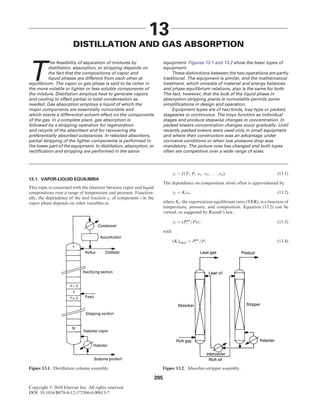
![where Psat
i is the vapor pressure of component I, and P is the system
total pressure. A number of correlations for VER have been de-
veloped for hydrocarbon systems that form relatively ideal solu-
tions, but for most chemical systems, Eq. (13.4) must be corrected.
At lower pressures (below about 5 atm), the correction factor is a
liquid phase activity coefficient gL
i (sometimes called a ‘‘Raoult’s
law correction factor’’).
A more rigorous expression is derived by noting that at equi-
librium, partial fugacities of each component are the same in each
phase, that is
f v
i ¼ f L
i (13:5)
or, in terms of fugacity and activity coefficients,
yifv
i P ¼ gL
i xifL
i Psat
i (13:6)
and the VER becomes
Ki ¼
yi
xi
¼
gL
i fsat
i Psat
i
fv
i P
(13:7)
Additionally, small corrections for pressure, called Poynting
factors, belong in Eq. (13.6) but are omitted here. The new terms
are:
fsat
i ¼ fugacity coefficient of the pure component at its vapor
pressure,
fv
i ¼ partial fugacity coefficient in the vapor phase.
Equations for fugacity coefficients are derived from equations
of state or are approximated from activity coefficient charts as
functions of reduced temperature and pressure. Table 13.1 includes
them for the popular Soave equation of state. At pressures below
5–6 atm, the ratio of activity coefficients in Eq. (13.7) often is near
unity. Then the VER becomes
Ki ¼ gL
i Psat
i =P (13:8)
which is independent of the nature of the vapor phase.
Values of the activity coefficients are deduced from experi-
mental data of vapor-liquid equilibria and correlated or extended
by any one of several available equations. Values also be calculated
approximately from structural group contributions by methods
called UNIFAC and ASOG. For more than two components, the
correlating equations favored nowadays are the Wilson, the
NRTL, and UNIQUAC, and for some applications a solubility
parameter method. The first and last of these are given in Table
13.2. Calculations from measured equilibrium compositions are
made with the rearranged equation
gi ¼
fu
i P
fsat
i Psat
i
yi
xi
(13:9)
’
P
Psat
i
yi
xi
: (13:10)
The last approximation usually may be made at pressures below
5–6 atm. Then the activity coefficient is determined by the vapor
pressure, the system pressure, and the measured equilibrium com-
positions.
Since the fugacity and activity coefficients are mathematically
complex functions of the compositions, finding corresponding
compositions of the two phases at equilibrium when the equations
are known requires solutions by trial. Suitable procedures for
making flash calculations are presented in the next section, and in
TABLE 13.1. The Soave Equation of State and Fugacity
Coefficients
Equation of State
P ¼
RT
V b
aa
V(V þ b)
z3
z2
þ (A B B2
)z AB ¼ 0
Parameters
a ¼ 0:42747R2
T2
c =Pc0
b ¼ 0:08664RTc =Pc
a ¼ [1 þ (0:48508 þ 1:55171! 0:15613!2
)(1 T0:5
r )]2
a ¼ 1:202 exp ( 0:30288Tr ) and for hydrogen
(Graboski and Daubert, 1979)
A ¼ aaP=R2
T2
¼ 0:42747aPr =T2
r
B ¼ bP=RT ¼ 0:08664Pr =Tr
Mixtures
aa ¼ SSyi yj (aa)ij
b ¼ Syi bi
A ¼ SSyi yj Aij
B ¼ Syi Bi
Cross parameters
(aa)ij ¼ (1 kij )
ffiffiffiffiffiffiffiffiffiffiffiffiffiffiffiffiffiffiffiffi
(aa)i (aa)j
p
kij in table
kij ¼ 0 for hydrocarbon pairs and hydrogen
Correlations in Terms of Absolute Differences between
Solubility Parameters of the Hydrocarbon, dHC and of the Inorganic
Gas
Gas kij
H2S 0:0178 þ 0:0244jdHC 8:80j
CO2 0:1294 0:0292jdHC 7:12j2
0:0222jdHC 7:12j2
N2 0:0836 þ 0:1055jdHC 4:44j 0:0100jdHC 4:44j2
Fugacity Coefficient of a Pure Substance
Inf¼ z 1 In z 1
b
V
aa
bRT
In 1 þ
b
V
¼ z 1 In(z B)
A
B
In 1 þ
B
z
Fugacity Coefficients in Mixtures
Infi¼
bi
b
(z 1) In z 1
b
V
þ
aa
bRT
bi
b
2
a
X
j
yj (aa)ij
#
In 1 þ
b
V
¼
Bi
B
(z 1) ¼ In(z B) þ
A
B
Bi
B
2
aa
X
j
yj (aa)ij
#
In 1 þ
B
2
(Walas, 1985).
396 DISTILLATION AND GAS ABSORPTION](data:image/gif;base64,R0lGODlhAQABAIAAAAAAAP///yH5BAEAAAAALAAAAAABAAEAAAIBRAA7)