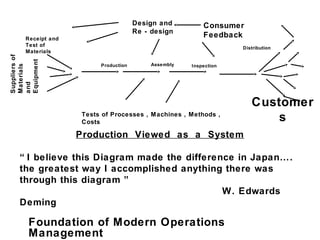
1. Design and Consumer
Re - design
Receipt and
Feedback
Test of Distribution
Materials
Suppliers of
Equipment
Assembly
Materials
Production Inspection
and
Customer
Tests of Processes , Machines , Methods ,
Costs s
Production Viewed as a System
“ I believe this Diagram made the difference in Japan….
the greatest way I accomplished anything there was
through this diagram ”
W. Edwards
Deming
Foundation of Modern Operations
Management
2. A META Group Study
Energy 30 crores per hour
Telecommunication 20 crores per hour
Manufacturing 17.5 crores per hour
Financial 15 crores per hour
Information Technology 15 crores per hour
Insurance 12.5 crores per
hour
Retail 10 crores per hour
Pharmaceutical 7.5 crores per hour
3. Evolution of Operations Management
Pre – Industrial Revolution Era
• Hunting
• Planned approach towards slaying and hunting living
creatures in defence or for consumption
• Agriculture
• Organising and coordinating groups of people to carry
out tasks in the fields
• Military Operations
• Regimented organisation of groups of people
established to protect a settlement from tyranny or
conquer
• Creation of Professions
• Essentially artisans who developed and passed on
‘trade secrets’ within their immediate families
• Handcrafting products or services for individual
customers
• Guilds
• Structured group of people involved with the same
4. Evolution of Operations Management
Industrial Revolution
Harnessing of Steam Energy
• James Watt
The First ‘Steam Engine’
• George Stevenson
The First Steam Machine
• Ginning Machines by Eli Whitney
Division of labour
• Economist Adam Smith conceives Division of
Labour
Interchangeable parts
• Eli Whitney invents interchangeability of parts
5. Evolution of Operations Management
Industrial Revolution
Principles of Scientific
Management
• Fredrick W. Taylor
Time and Motion Studies
• Frank and Lillian Gilbreth
Activity Scheduling
• Henry Gantt
The Moving Assembly Line
• Henry Ford
6. Evolution of Operations Management
The Focus
• Work Breakdown Structures
• One best Way of carrying out Processes
• Piece Rate System
The Outcomes
• The Meteoric Rise of Financial Accounting
• Extensive interest in Advertising and Branding
The rise of Motivational Theorists
• Elton Mayo
• Abraham Maslow
• Fredrick Herzberg
• Douglas McGregor
7. Evolution of Operations Management
The Return of
Operations
The Quality Revolution in Japan
• W. Edwards Deming and Joseph M. Juran
The Development of the Toyota Production System
• Eigi Toyoda , Taichi Ohno and Shiego Shengo
Modern Trends in Operations
• Business Process Reengineering
• Six Sigma
8. Operations in Today’s
World
The Internet Revolution
•E – Commerce
•E – Businesses
B2B
OEMs or ‘First Fit’ Businesses
B2C
Franchises
C2B
Consultation
C2C
eBay,Portals,etc
Globalisation of trade
Globalisation of Operations ( Development of the
Virtual Organisation )
9. Definition of Operations Management
Operations Management is the system of Selecting ,
Designing , Running and Improving all transformational
processes
Transformational processes
include :
Governmental – Creating and Running Societal
Structures
Physical – Manufacturing
Exchange – Retail Operations , Banks
Locational – Logistics and Transportation
Physiological – Healthcare and Hospitality
Psychological – Entertainment
Informational – Communication , Interpretation
Educational – Structured Knowledge Transfer
Production is the outcome of the combination of different
transformational processes ( operations ) aimed at meeting
desired Customer needs .
Production Management aims at achieving Production in
the most efficient and effective manner .
10. Organisation
s
Governmental
Physica
l
Exchange
s
Locationa
l
Processes
Operation
Transformational
Physiological
Psychologica
l
Informationa
l
Educational
Productio
n
11. The Need for Operations Management in
today’s World
In the ever changing Business Scenario in today’s
fast developing world where we are witnessing
• Incessant Fragmentation of Markets
• Highly Informed and Vocal Customers
• Creation of Disruptive Technologies resulting in
Specialised Knowledge
• Volatile Inter – Organisational Relationships
12. Objectives of Operations
Management
Strategy – Gaining a Competitive Edge
Processes and Systems – Alignment of Back-
end activities
Quality – Scientific Methods to Create and
Deliver Products / Services
Improvement – A Constant effort to challenge
the Status Quo / Obvious
13. • Topic 1 – Introduction to Operations Management
• Topic 2 – Facility Location
• Topic 3 – Facility ( Plant ) Layout
• Topic 4 – Production Planning and Control
• Topic 5 – Materials Handling
• Topic 6 – Work Study
• Topic 7 – Systematic Maintenance
• Topic 8 – Quality Management
• Topic 9 – Modern Techniques in Operations Management
14. Regional Location Factors
• Busine ss climate
• Proximity to customers
• Numbe r of customers
• Availab ility of sites
• Land cost
• Constr uction / leasin g costs
• Infrastructure (e.g., roads , water, sewer s)
• Financial service s
• Community incent ives
• Community services
• Govern menta l Incent ive
• Govern ment regula tions
• Environ mental regula tions
15. Regional Location
Factors
• Labour (availability, education, cost, and unions)
• Modes and Quality of transportation
• Transportation costs
• Local business regulations
• Government services (e.g., Chamber of
Commerce)
• Raw material availability
• Commercial travel
• Climate
• Quality of life
• Taxes
• Proximity of suppliers
• Education system
16. Global Location
Factors
• Government stability
• Government regulations
• Political and economic systems
• Economic stability and growth
• Exchange rates
• Culture
• Climate
• Export import regulations
• Duties and tariffs
• Raw material availability
• Number and proximity of suppliers
17. Global Location
Factors
• Transportation and distribution system
• Labour cost and education
• Available technology
• Commercial travel
• Technical expertise
• Cross-border trade regulations
• Group trade agreements
18. Types of
Facilities
Heavy-manufacturing facilities
Large, require a lot of space, and are expensive
Light-industry facilities
Smaller ( as compared to Large Industries ),
cleaner plants and usually less costly
Retail and service facilities
Smallest and least costly
19. Location Analysis
Techniques
Multiattribute Preference Theory ( Location
Rating Factor ) for Local Sites
• Is used when choices are available
• Has no ‘scientific’ basis – just an ‘agreed upon’
weighted technique
Attribute Weight
Labour Force 0.30
Proximity to 0.20
Customers
Wage Rates 0.15
Proximity to 0.15
Suppliers
Environment 0.10
Modes of Transport 0.05
Community Support 0.05
20. Location Analysis
Techniques
Guidelines for Scores :
Labour Force
75 –
Highly Skilled 100
50 –
Adequately Skilled
75
25 –
Semi Skilled 50
Unskilled 0 – 25
21. Location Analysis
Techniques
Guidelines for Scores :
Proximity to Customers
75 –
Within 15 kilometres
100
Between 15 to 30 50 –
kilometres 75
Between 30 to 50 25 –
kilometres 50
Above 50 kilometres 0 – 25
22. Location Analysis
Techniques
Guidelines for Scores :
Wage Rates
75 –
Upto 10 % of total cost
100
Between 10 – 15 % of total 50 –
cost 75
Between 15 – 20 % of total 25 –
cost 50
Above 20 % of total cost 0 – 25
23. Location Analysis
Techniques
Guidelines for Scores :
Proximity to Suppliers
75 –
Within 15 kilometres
100
Between 15 to 30 50 –
kilometres 75
Between 30 to 50 25 –
kilometres 50
Above 50 kilometres 0 – 25
24. Location Analysis Techniques
Guidelines for Scores :
Environment
75 –
Conducive to Ceaseless Productive Work
100
50 –
Conducive to Productive Work over 25 % 75
25 –
Conducive to Productive Work for a day
50
Conducive to Productive Work for less
0 – 25
than a day
25. Location Analysis
Techniques
Guidelines for Scores :
Modes of Transport
Access to any two modes of transport at 75 –
any given moment 100
Access to any one mode of transport at 50 –
any given moment 75
Need to plan a day in advance for any 25 –
mode of transport 50
Need to plan more than a day in advance
0 – 25
for any mode of transport
26. Location Analysis
Techniques
Guidelines for Scores :
Community Support
Extremely harmonious relationships with 75 –
communities in close proximity 100
Have Legal relationships with 50 –
communities in close proximity 75
Have dispassionate relationships with 25 –
communities in close proximity 50
Have hostile relationships with
0 – 25
communities in close proximity
27. Exampl
e
A company wanting to relocate its operations has assessed
three sites and have tabulated the following results
Attribute Site 1 Site 2 Site 3
Labour Force 70 60 90
Proximity to
80 90 75
Customers
Wage Rates 60 95 70
Proximity to 75 80 80
Suppliers
Environment 65 90 95
Modes of Transport 85 90 65
Community Support 80 65 90
Which Site qualifies based on the Multiattribute Preference
Theory ?
28. Using Weights ascribed we
get
Wei Si Sit Sit
Attribute
ght te 1 e 2 e 3
0.3
Labour Force 70 60 90
0
Proximity to 0.2 80 90 75
Customers 0
0.1
Wage Rates 60 95 70
5
Proximity to 0.1 75 80 80
Suppliers 5
0.1
Environment 65 90 95
0
29. Weighted
Scores
Scores : Site 1 – 72.00 ; Site 2 – 79.00 ; Site 3
– 81.75
Attribute Site 1 Site 2 Site 3
Labour Force 21.00 18.00 27.00
Proximity to 16.00 18.00 15.00
Customers
Wage Rates 9.00 14.25 10.50
Proximity to
11.25 12.00 12.00
Suppliers
Environment 6.50 9.00 9.50
Modes of 4.25 4.50 3.25
Transport
Site 3 – The preferred
Community
location 4.00 3.25 4.50
30. Typical Attributes that an MNC looks for in a
Global Operations Site
Attribute Weight
Political Stability 0.25
Economic Growth 0.20
Port Facilities 0.13
Airline Support 0.10
Trade Regulations 0.08
Duties and Tariffs 0.08
Container Support 0.07
Transportation / 0.05
Distribution
Area Roads 0.02
31. Centre of Gravity Technique
Normally used in computing location of sites for
Warehouses / Distribution Centres
Current Location is set as ( 0 , 0 ) on a Cartesian
Plane
Average Annual Despatch Loads to different sites
are indicated in parenthesis
Distribution Site co-ordinates are computed
accordingly
A Pictorial Representation in the form of a Graph
is drawn
32. y
2 (x 2 , y 2 ),
y2
W2
1 (x 1 , y 1 ),
y1 W1
3 (x 3 , y 3 ),
y3
W3
x1 x2 x3
x
Current Site of
Operations
34. Example
A B C D
y x 200 100 250 500
y 200 500 600 300
700
Wt 70 100 130
C
60
600 (130)
B
500 (100)
Kilometres
400
D
300 (60)
A
200 (70)
100
0 100 200 300 400 500 600 700 x
Kilometres
35. Co-ordinates of New Location ( x , y ) are computed
thus
(200)(70) + (100)(100) + (250)(130) +
x= = 240
(500)(60)
70 + 100 + 130+ 60
(200)(70) + (500)(100) + (600)(130) +
y= = 444
(300)(60)
70 + 100 + 130+ 60
36. Location of the Warehouse
y
70
0 C
60 (130)
0 B (100)
Kilometre
50 ( 240 , 444 )
0
40
0 D
s
30 (60)
0 A
200 (70)
10
0
x
0 100 20 30 40 50 60 70
0 0 Kilometre
0 0 0 0
s
37. Load Distance
Technique
Variation of the Centre of Gravity
Technique
Used when Options available for Sites
Use of the Straight Line concept ( Based on Geometric Distance
Formula )
n
LD =
∑ li di
i= 1
LD = load-distance value
li = load expressed as a weight being despatched
di = distance between proposed site and
location i
di = (x i - x) 2 + (y i - (x,y) = coordinates of proposed site
y) 2
(x i , y i) = coordinates of existing facility
38. Suppliers
A B C
D
x 200 100 250
500
y 200 500 600
300Potential Sites
Wt Site X100 130
70 Y
601 360 180
2 420 450
3 250 400
39. A B C D Potential Sites
x 200 100 250 500 Site X Y
y 200 500 600 300 1 360 180
Wt 70 100 130 2 420 450
60 3 250 400
Computing distances for Site 1
dC = (x C - x 1 ) 2 + (y C - y 1 ) 2
dA = (x A - x 1 ) 2 + (y A - y 1 ) 2
= (250-360) 2 + (600-180) 2
= (200-360) 2 + (200-180) 2
= 434.16
= 161.2
dB = (x B - x 1 ) + (y B - y 1 )
2 2 dD = (x D - x 1 ) 2 + (y D - y 1 ) 2
= (100-360) + (500-180)
2 2 = (500-360) 2 + (300-180) 2
= 412.3 = 184.31
Load Distance =
(70)*(161.2)+(100)*(412.3)+(130)*(434.16)+(60)*(184.31)
=
120019.2
40. A B C D Potential Sites
x 200 100 250 500 Site X Y
y 200 500 600 300 1 360 180
Wt 70 100 130 2 420 450
60 3 250 400
Computing for Site 2
dC = (xC – x2)2 + (yC – y2)2
dA = (xA – x2)2 + (yA – y2)2
= (250-420)2 + (600-450)2
= (200-420)2 + (200-450)2
= 333.02 = 226.71
dB = (xB – x2)2 + (yB – y2)2 dD = (xD – x2)2 + (yD – y2)2
= (100-420) + (500-450)
2 2 = (500-420)2 + (300-450)2
= 323.88 = 170
Load Distance = (70)*(333.02)+(100)*(323.88)+(130)*(226.71)+(60)*(170)
= 97036.8
41. A B C D Potential Sites
x 200 100 250 500 Site X Y
y 200 500 600 300 1 360 180
Wt 70 100 130 2 420 450
60 3 250 400
Computing for Site 3
dA = (xA – x3)2 + (yA – y3)2 dC = (xC – x3)2 + (yC – y3)2
= (200-250)2 + (200-400)2 = (250-250)2 + (600-400)2
= 206.19 = 200
dB = (xB – x3) + (yB – y3)
2 2 dD = (xD – x3)2 + (yD – y3)2
= (100-250)2 + (500-400)2 = (500-250)2 + (300-400)2
= 180.27 = 269.25
Load Distance = (70)*(206.19)+(100)*(180.27)+(130)*(200)+(60)*(269.25)
= 74614.8
42. Facility Layouts
Definition of Facility
Layout
Planned arrangement of areas within a facility
commensurate with the product to be realised or
service to be delivered
Objectives of Facility
Layout
• Optimise material-handling ( transaction ) costs
• Utilise space efficiently
• Utilise manpowe r efficiently
• Work around bottlenecks
• Facilitate interaction
• Reduce cycle time
• Reduce customer turnaround time
• Eliminate redundant movement
• Increase capacity
• Provide for entries, exits, placement of material ( in all
stages of realisation ), finished goods, and people
43. Facility Layouts
Objectives of Facility Layout ( continued )
• Incorporate safety and security measures
• Promote product and service Quality
• Facilitate proper maintenance activities
• Provide for visual control
• Provide for flexibility to adapt to changing conditions
44. Different Organisational Layout
Representations
• Departmental Layout
• Material Flow Layout
• Equipment Layout
• Transportation and Handling Layout
• Utilities Layout
• Communication Channel Layout
45. Basic Types of Layouts
Fixed-position layouts
are used where product cannot be moved
Used for Large Products and Projects
Usually ‘one-of-a-kind’ products or projects
Process layouts
group similar activities together according to process or
function they perform
Traditional Type of Layout
Suitable for Mass Production
Product layouts
arrange activities in line according to sequence of
operations for a particular product or service
Modern Approach toward Creating Layouts
More inclined towards Mass Customisation
46. Fixed-position layouts
Typically manufacture of Construction Projects ,
Rocket Launchers , Space Shuttles , Aircrafts ,
Ships , Surgeries , “Events”
Equipment, workers, materials, other resources
brought to site
Highly skilled labour
47. Process Layout - Bookstore
Video CDs Audio CDs ,
Cassettes
, DVDs DVDs
Technical
Cookbooks Billing and and
Information Management
Section
Children’s Entry and Coffee
Books display area Shop
48. Process Layout - Manufacture
Lathe Section Milling Section Drilling Section
M M D D D D
L L
M M D D D D
L L
G G G P
L L
G G G P
L L
Painting Department
Grinding and Finishing
L L
Receiving and A A A
Shipping Assembly
Product A Product B
49. Product Layout - Manufacture
In Out
Product A
In Out
Product B
In Out
Product C
50. Comparisons between Product and Process Layouts
Product Layout Process Layout
• Sequential arrangement of • Functional Grouping of
Activities Activities
• Intermittent work • Continuous work
• Adaptable Machinery • General Purpose Machinery
• Workers are extensively cross- • Workers are trained in a
trained particular process
• Occupy smaller areas • Occupy larger areas
• Highly flexible lines • Largely Rigid
• Lesser travel time • More travel time
51. Designing Layouts
Relationship Diagramming
• based on location preference between areas
• used when quantitative data is not available
• Schematic diagram that uses weighted lines
to denote location preference
Use of a grid called “Muther’s grid”
53. A Absolutely necessary
E Especially important
I Important
O Okay
U Unimportant
X Undesirable
Production
O
Offices A
U I
Stockroom O E
A X A
Shipping and receiving U U
U O
Locker room O
O
Toolroom
54. Original layout
Offices Locker Shipping
room and
receiving
Stockroom Toolroo Production
m
A
E
I
O
U
X
55. Relationship diagram of original layout
Offices Locker Shipping and
room receiving
A
E
Stockroom Toolroom Production I
O
U
X
56. Production – 2 ‘Absolutely Necessary’ transactions ;
1 ‘Especially Important’ transaction ;
1 ‘Important’ transaction ;
1 ‘Okay’ transaction
Therefore Production needs to be centrally located
with the other departments around it .
57. Solution 1 A
E
I
O
U
Stockroom X
Offices
Shipping and
receiving
Toolroom
Production Locker room
58. Solution 2 A
E
I
O
U
Stockroom X
Locker room
Offices
Shipping and Production Toolroom
receiving
59. Block Diagramming
Purpose is to minimise nonadjacent loads
Used when quantitative data is available
Steps :
• Create load summary chart
• Calculate composite (two way) movements
• Develop trial layouts minimising number
of nonadjacent loads
65. Cellular Layouts
Identify outputs with similar flow paths
Group processes into cells based on output
Arrange cells so transactions are minimised
Locate shared processes at point of use
68. Determine Flow Logic
A : 1 – 2 – 4 – 8 – 10
B : 5 – 7 – 11 – 12
C:3–6–9
D : 1 – 2 – 4 – 8 – 10
E : 5 – 6 – 12
F:1–4–8
G : 3 – 6 – 9 – 12
H : 7 – 11 – 12
69. Part Routing Matrix
Workstations
Pro V
ducts 1 1 1 alue
1 2 3 4 5 6 7 8 9
0 1 2
A X X X X X
B X X X X
C X X X
D X X X X X
E X X X
F X X X
G X X X X
H X X X
Valu
e
70. Create Binary Algorithm
The procedure works like this :
• Assign a value to each column ‘k’ , where the
value is 2 N-k N = total number of workstations ; k =
chronological workstation number
• For each row obtain a sum by adding the 2 N-k
values
• Rearrange the rows in the decreasing order of the
sums obtained
• Assign a value to each row ‘k’ where the value is
2 M-k M = total number of products ; k =
chronological ( rearranged ) sequence number of
the product
• For each column obtain a sum by adding the
values
• Rearrange the columns in decreasing order of the
sums obtained
71. Part Routing Matrix
Workstations
Pro V
ducts 1 1 1 alue
1 2 3 4 5 6 7 8 9
0 1 2
2 1 2 1 3
A 048 024 56 6
4
348
1 3 1
B 28 2
2 1
63
5 6 5
C 12 4
8
84
2 1 2 1 3
D 048 024 56 6
4
348
1 6 1
E 28 4
1
93
2 2 1 2
F 048 56 6 320
5 6 5
G 12 4
8 1
72. Part Routing Matrix
Workstations
Pro V
ducts 1 1 1 alue
1 2 3 4 5 6 7 8 9
0 1 2
2 1 2 1 3
A 048 024 56 6
4
348
2 1 2 1 3
D 048 024 56 6
4
348
2 2 1 2
F 048 56 6 320
5 6 5
G 12 4
8 1
85
5 6 5
C 12 4
8
84
1 6 1
E 28 4
1
93
1 3 1
B 28 2
2 1
73. Part Routing Matrix
Workstations
Pro V
ducts 1 1 1 alue
1 2 3 4 5 6 7 8 9
0 1 2
A X X X X X
D X X X X X
F X X X
G X X X X
C X X X
E X X X
B X X X X
H X X X
Valu
e
74. Part Routing Matrix
Workstations
Pro V
ducts 1 1 1 alue
1 2 3 4 5 6 7 8 9
0 1 2
1 1 1 1 1
A
28 28 28 28 28
6 6 6 6 6
D
4 4 4 4 4
3 3 3
F
2 2 2
1 1 1 1
G
6 6 6 6
C 8 8 8
E 4 4 4
B 2 2 2 2
H 1 1 1
Valu 2 1 2 2 2 2 2 1 2
75. Part Routing Matrix
Workstations
Pro V
ducts 1 1 1 alue
1 4 8 2 6 3 9 5 7
0 2 1
1 1 1 1 1
A
28 28 28 28 28
6 6 6 6 6
D
4 4 4 4 4
3 3 3
F
2 2 2
1 1 1 1
G
6 6 6 6
C 8 8 8
E 4 4 4
B 2 2 2 2
H 1 1 1
76. Part Routing Matrix
Workstations
Prod
ucts 1 1 1
1 4 8 2 6 3 9 5 7
0 2 1
A X X X X X
D X X X X X
F X X X
G X X X X
C X X X
E X X X
B X X X X
H X X X
77. Part Routing Matrix
Workstations
Prod
ucts 1 1 1
1 4 8 2 6 3 9 5 7
0 2 1
A X X X X X
D X X X X X
F X X X
G X X X X
C X X X
E X X X
B X X X X
H X X X
78. Revised Layout
Outputs
8 10 9 12
11
4 Cell 1 Cell 2 6 Cell 3
7
2 1 3 5
A B C
Inputs
89. Direction of part movement within cell
HM
VM
Worker 3
Paths of three workers VM
moving within cell
L
Material movement
Worker 2
S = Saw G
L = Lathe
HM = Horizontal milling machine L
VM = Vertical milling machine
G = Grinder Final
inspection
Finished
part
S Worker 1
Out
In
90. Service Layouts
• Usually process layouts respond to
customer needs
• Minimise flow of customers or
transactions
• Retailing tries to maximise customer
exposure to products
• Layouts must be aesthetically pleasing
95. Types of Production Processes
Criteria for Selection of Processes
Nature of the Inputs and Outputs
Perishable and Non – Perishable
Quantum of Production
One – of
Few Numbers
Mass
Nature of Operations
Continuous Processes
Intermittent Processes
Capacity of the Plant
Restrictions in Space , Equipment , Labour , Technology
96. Types of Production Processes
Types of Processes
Jobbing / Project Type Method
This method is used where , although the Processes
remain the same , the outputs are unique in nature .
Example : Construction Projects , Film Making , Job
Shops
Features of this Approach
• One – of or Very Small Quantity of Production
• Highly Skilled Workforce
• General Purpose Equipment
• Unbalanced Processing
• High Cost of Production
97. Types of Production Processes
Types of Processes
Batch Type Approach
This method is used where a limited amount of products
( batches ) are produced at a time either continuously or
intermittently .
Example : Chemicals , Pharmaceuticals , Paints , Foods
and some types of metal items
Features of this Approach
• Fixed Quantities Produced
• Semi – Skilled Workforce
• General Purpose Equipment
• Balanced Processing
• Low Cost of Production
98. Types of Production Processes
Types of Processes
Mass Production
This method is used where a very large amount of
products ( batches ) are produced at a time either
continuously .
Example : Engineered Products , Fertilisers
Features of this Approach
• Very Large Quantities Produced
• Semi – Skilled Workforce
• General Purpose Equipment
• Very High Flows
• Low Cost of Production
99. Types of Production Processes
Types of Processes
Process Based Production
This method is used where Bulk items are produced
Example : Sugar , Aluminium , Zinc , Iron and Steel
Features of this Approach
• Bulk Items Produced
• Semi – Skilled Workforce
• General Purpose Equipment
• Very High Flows
• Low Cost of Production
100. Ways of Doing Work
PRODUCT MIX
One of Low Volume High Volume Mass
Project Job
Jumbled
Shop
PROCESS PATTERN
Jumbled But
Batch
Dominant
K
Line
Line Flow
Continuous Continuous
Flow
101. Production Planning and Control
Introduction
• Coordination of materials function
with suppliers
• Efficient utilisation of people and
machines
• Efficient flow of materials within the
organisation
102. The “Seepok” Model
Production
Inputs Outputs
Suppliers Customers
S I P O C
103. Decision Support
• PPC system does not make decisions
but provides support for decision
making
• Managers make decisions
104. Software for Decision Support
• Software not only to support decision
makers but also make some of the
decisions
• Expert Systems
• Neural Networks
• Algorithms
• Evolutionary Programming
• Genetic Programming
• Tabu Search
• Simulated Annealing
105. Activities
• Materials Planning
• Purchasing
• Raw Material Inventory Control
• Capacity Planning
• Scheduling Machine and People
• Work-in-Process (WIP) Inventory
Control
• Coordinate Customer Orders
• Finished Goods Inventory Control
106. Ill-effects of a lack of PPC
• poor customer service
• excessive inventories
• low equipment and people utilisation
• high rate of part obsolescence
• large number of expediters
107. Specification Inventory
Work Study
s Management
Production Planning and Control
Routing Loading Scheduling Despatching Expediting
Production Plan
108. Routing
• Determine the Processes to be followed
• Determine the Sequence of the Processes
• Determine the Flow of Materials / Activities
109. Loading
• Determine the Number of Workstations
• Determine their operational characteristics ( speeds ,
capabilities )
• Selection of Workstations
• Creating a Contingency Plan
110. Scheduling
• Determining the exact time at which the Operations
will materialise
• Timing the arrival of material ( finished / semi-finished
part at different workstations )
• Usually done on a ‘Gantt Chart’
113. Production Planning and Control
General Framework
Resources Demand
Planning Management
Rough-Cut Capacity
Planning Master Production Scheduling
Detailed Capacity Detailed Material
Planning Planning
Material and
Capacity Plans
Work Order Purchase
Order
114. Demand Management
• Forecasting
• Order Processing
• Order Acceptance
• Order Confirmation
115. Resource Planning
• Long-Range Capacity Requirements
• Number of Plants
• Number of Workstations
• Number of Employees
• Shifts
• Overtime
116. Production Planning
Plans for Product Families
Master Planning Schedule ( MPS )
Anatomy of a Plan
Annual Plan
Quarterly Plan
Monthly Plan
Fortnightly Plan
Fixed Could be subject to minor changes
118. Detailed Materials Planning
Materials Requirements Planning
Inputs :
• Master Production Schedule (MPS)
• Bill of Materials (BOM)
• Inventory Status
• Leadtime (LT)
119. Bill of Material (BOM)
Shows the constituent components and how
many of those are required to build the
composite part
120. Product Structures and Parts
C Finished Product
Manufactured
Part
A Sub Assembly B
X X Y
Purchased Parts
121. Single Level Bill of Material
2 units of component X are used to make 1 unit of item A
Level 0 Parent A
Level 1 Component X X2
Indented Bill of Material ( BOM ) for A is
Lev Part ( nos
el )
0 A( 1 )
1 X ( 2 )
122. Single Level Bill of Material
2 units of component X and 1 component of Y are used to
make 1 unit of item B
Level 0 Parent B
Level 1 Component X X2
Level 1 Component Y X1
Indented Bill of Material ( BOM ) for B is
Lev
Part ( nos )
el
0 B(1)
1 X(2)
1 Y(1)
123. Single Level Bill of Material
Level 0 Parent C
Level 1 Component A X2
Level 1 Component B X3
2 units of component A and 3 components of B are used to
make 1 unit of item C
Indented Bill of Material ( BOM ) for C is
Lev
Part ( nos )
el
0 C(1)
1 A(2)
1 B(3)
124. Multi Level Bill of Material
Level 0 Parent C
Level 1 2xA 3xB
Level 2 2xX 2xX 1xY
125. Summary Bill of Material
Cumulati Summary BOM for C
Level Part
ve
0 C 1
1 A 2 X 10
2 X 4 Y 3
1 B 3
2 X 6
2 Y 3
126. Create a BOM for a Two layered McDonald’s
Maharaja Mac
Sesame Seed Top bun
Bottom Bun Sub Assembly Middle Bun Sub Assembly
Bottom Bun Patty Sauce Lettuce Cheese Patty Onions
Middle Bun
127. Inventory Status
On Hand (OH) Quantity
What is physically available in the warehouse
On Order or Scheduled Receipt (SR)
What has been ordered but not received ( transitory )
Allocated Inventory (AI)
What is in the warehouse but reserved for existing
orders (i.e., not available to be used for incoming
orders)
128. Leadtime
Time between placing an order and receiving the parts
Parts could be
• Purchased – Dependant on Vendor
• Manufactured or assembled in house – Dependant
on Process / Manufacturing Personnel
129. Leadtime Offsetting
1.Front Schedule Approach
Schedule as early as possible
Advantage: Minimise risk of shortage
Disadvantage: Higher Inventory Levels
2.Back Schedule Approach
Schedule as late as possible
Advantage: Minimise Inventory
Disadvantage: Higher Risk of Shortage
130. Important Terms / Conventions used in MRP
Gross Requirements – Derived from the MPS of the Parent
Part
Scheduled Receipts – On Order or Scheduled to be
received
On Hand – Physical Available Inventory
Allocated Inventory – Inventory scheduled to be used
Nett Requirements – Actual Quantities Required
Planned Order Receipts – Offset time when Materials are
needed
Planned Order Releases – Offset Time when materials need
to be ordered ( function of lead time )
131. MRP Matrix
Week Number
Heading
1 2 3 4 5
Gross 12 10 10
85 95
Requirements 0 0 0
Scheduled 17
Receipts 5
On Hand 45
Allocated Inventory 20
Nett Requirements
Planned Order
Receipts
Planned Order
Releases
132. MRP Matrix
Week Number
Heading
1 2 3 4 5
Gross 12 10 10
85 95
Requirements 0 0 0
Scheduled 17
Receipts 5
11
On Hand 45
5
Allocated Inventory 20
Nett Requirements 0
Planned Order
Receipts
Planned Order
133. MRP Matrix
Week Number
Heading
1 2 3 4 5
Gross 12 10 10
85 95
Requirements 0 0 0
Scheduled 17
Receipts 5
11
On Hand 45 20
5
Allocated Inventory 20
Nett Requirements 0 0
Planned Order
Receipts
Planned Order
139. Scheduling
Last stage of planning before production
occurs
Specifies when labour, equipment, facilities
are needed to produce a product or provide
a service
140. Objectives in Scheduling
Meet customer due dates
Minimise response time
Minimise completion time
Minimise time in the system
Minimise overtime
Minimise work-in-process inventory
141. Shop Floor Control
Loading
Check availability of material, machines and labour
Sequencing
Release work orders to shop and issue despatch
lists for individual machines
Monitoring
Maintain progress reports on each job until it is
complete
143. Assignment Method
Perform row reductions
subtract minimum value in each row from all other row
values
Perform column reductions
subtract minimum value in each column from all other
column values
Cross out all zeros in matrix
use minimum number of horizontal and vertical lines to
cover all the 0s
If number of lines equals number of rows in matrix then
optimum solution has been found. Make assignments where
zeros appear
Else modify matrix
subtract minimum uncrossed value from all uncrossed
values
add it to all cells where two lines intersect
other values in matrix remain unchanged
Repeat steps 3 through 5 until optimum solution is reached
144. Example
Time taken for completing
Name the task
1 2 3 4
Duryodh
an
10 5 6 10
Dushyas
an
6 2 4 6
Jarasan
dha
7 6 5 6
Jayadra
tha
9 5 4 10
145. Step 1 - Row Reduction
Time taken for completing
Name the task
1 2 3 4
Duryodh
an
5 0 1 5
Dushyas
an
4 0 2 4
Jarasan
dha
2 1 0 1
Jayadra
tha
5 1 0 6
146. Step 2 - Column Reduction
Time taken for completing
Name the task
1 2 3 4
Duryodh
an
3 0 1 4
Dushyas
an
2 0 2 3
Jarasan
dha
0 1 0 0
Jayadra
tha
3 1 0 5
147. Step 3 - Cover all Zeros
Time taken for completing
Name the task
1 2 3 4
Duryodh
an
3 0 1 4
Dushyas
an
2 0 2 3
Jarasan
dha
0 1 0 0
Jayadra
Number of Lines = 3 ; Number of Rows = 4
tha
3 1 0 5
Modify Matrix
148. Step 4 - Modify the Matrix
Time taken for completing
Name the task
1 2 3 4
Duryod
3 0 1 4
han
Dushy
2 0 2 3
asan
Jarasa
0 1 0 0
ndha
Jayadr
3 1 0 5
atha
Take the lowest value in the ‘uncovered’ cells ( in this
case = 2 ) and reduce the column to which it belongs
Add this value to the values of the intersecting cells
as shown
149. Step 5 - Select the
Tasks
Time taken for completing
Name the task
1 2 3 4
Duryodh
an
1 0 1 4
Dushyas
an
0 0 2 3
Jarasan
dha
0 3 2 0
Jayadra
tha
1 1 0 5
150. Example
Time taken for completing
Name the task
1 2 3 4
Duryodh
an
10 5 6 10
Dushyas
an
6 2 4 6
Jarasan
dha
7 6 5 6
Jayadra
tha
9 5 4 10
151. Example
Time taken for completing
Name the task
1 2 3 4
Savani 20 90 40 10
Vidheya 40 45 50 35
Antara 30 70 35 25
Amala 60 45 70 40
152. Step 1 - Row Reduction
Time taken for completing
Name the task
1 2 3 4
Savani 10 80 30 0
Vidheya 5 10 15 0
Antara 5 45 10 0
Amala 20 5 30 0
153. Step 2 - Column Reduction
Time taken for completing
Name the task
1 2 3 4
Savani 5 75 20 0
Vidheya 0 5 5 0
Antara 0 40 0 0
Amala 15 0 20 0
154. Step 3 - Cover all Zeros
Time taken for completing
Name the task
1 2 3 4
Savani 5 75 20 0
Vidheya 0 5 5 0
Antara 0 40 0 0
Amala 15 0 20 0
Number of lines = Number of Rows
155. Step 4 - Select the
Tasks
Time taken for completing
Name the task
1 2 3 4
Savani 5 75 20 0
Vidheya 0 5 5 0
Antara 0 40 0 0
Amala 15 0 20 0
156. Step 5 - Assign
Jobs
Time taken for completing
Name the task
1 2 3 4
Savani 20 90 40 10
Vidheya 40 45 50 35
Antara 30 70 35 25
Amala 60 45 70 40
158. Sequencing Rules
FCFS - first-come, first-served
LCFS - last come, first served
DDATE - earliest due date
CUSTPR - highest customer priority
SETUP - similar required setups
SLACK - smallest slack
CR - critical ratio
SPT - shortest processing time
LPT - longest processing time
159. Sequencing Jobs Through Two Serial
Processes
Johnson’s Rule
List time required to process each job at each machine. Set
up a one-dimensional matrix to represent desired sequence
with number of slots equal to number of jobs.
Select smallest processing time at either machine. If that
time is on machine 1, put the job as near to beginning of
sequence as possible.
If smallest time occurs on machine 2, put the job as near to
the end of the sequence as possible.
Remove job from list.
Repeat steps 2-4 until all slots in matrix are filled and all
jobs are sequenced.
160. Johnson’s Rule
Jobs
Machi
nes A B C D E F
M1 4 8 3 6 7 5
M2 6 3 7 2 8 4
C A F E B D
161. 1 2 3 4 5 6 7 8 9 1 1 1 1 1 1 1 1 1 1 2 2 2 2 2 2 2 2 2 2 3 3 3 3 3
0 1 2 3 4 5 6 7 8 9 0 1 2 3 4 5 6 7 8 9 0 1 2 3 4 5
Machi C A F E B D
ne 1
Machi C A F E B D
ne 2
162. Example
Jobs
Machin
es
A B C D E
M1 10 12 8 15 16
M2 3 2 4 1 5
M3 5 6 4 7 3
M4 14 7 12 8 10
C A E D B
163. Machin Machin Machin Machine
IDLE TIME
Sequenc e1 e2 e3 4
e I O I O I O I O M M M M
N UT N UT N UT N UT 1 2 3 4
1 1 1 1 1
C 0 8 8 16 28 - 8
2 2 6 2 6
1 1 2 2 2
A 8 26 42 - 6 5 -
8 8 1 1 8
1 3 3 3 3 4 1 1
E 42 52 - -
8 4 4 9 9 2 3 3
3 4 4 5 5 5 1
D 57 65 - 8 5
4 9 9 0 0 7 0
4 6 6 6 6 6 1
B 69 76 - 6 4
9 1 1 3 3 9 1
N 4 4 2
IL 8 4 5
164. The Heuristic Method
Jobs
Machines
A B C D
M1 4 3 1 3
M2 3 7 2 4
M3 7 2 4 3
M4 8 5 7 2
Add the time taken on Machines 1 and 2 to create a
‘new’ Machine
Compute similarly for Machines 3 and 4
165. Example
Jobs
Machi
nes
A B C D
M1 7 10 3 7
M2 15 7 11 5
C A B D
166. Machin Machin Machin Machine
IDLE TIME
Sequ e1 e2 e3 4
ence I O I O I O I OU M M M M
N UT N UT N UT N T 1 2 3 4
C 0 1 1 3 3 7 7 14 - 1 3 7
1
A 1 5 5 8 8 15 23 - 2 1 1
5
1 1 2
B 5 8 8 17 28 - - - -
5 5 3
1 1 1 1 2
D 8 22 30 - - 2 -
1 5 9 9 8
N
3 6 8
IL
167. Example
The following 6 jobs have the following Processing Times and
Due Dates . Compare which of the following sequencing
methods will be best suited for these jobs : FCFS , LCFS ,
DDATE , SPT
J Process Due Date
obs ing Time ( from now )
A 2 6
B 5 9
C 3 8
D 4 12
E 1 10
F 7 11
G 6 13
168. Solution
FCFS – First Come First Served
Due
Job Processin Total
Date ( from Delay
s g Time Flow Time
now )
A 2 6 2 0
B 5 9 7 0
C 3 8 10 2
D 4 12 14 2
E 1 10 15 5
F 7 11 22 11
G 6 13 28 15
Average Flow Time = 14
Average Delay = 5
169. Solution
LCFS – Last Come First Served
Due
Job Processin Total
Date ( from Delay
s g Time Flow Time
now )
G 6 13 6 0
F 7 11 13 2
E 1 10 14 4
D 4 12 18 6
C 3 8 21 13
B 5 9 26 17
A 2 6 28 22
Average Flow Time = 18
Average Delay = 9.14
170. Solution
DDATE – Earliest Due Date
Due
Job Processin Total
Date ( from Delay
s g Time Flow Time
now )
A 2 6 2 0
C 3 8 5 0
B 5 9 10 1
E 1 10 11 1
F 7 11 18 7
D 4 12 22 10
G 6 13 28 15
Average Flow Time = 13.7
Average Delay = 4.85
171. Solution
SPT – Shortest Processing Time
Due
Job Processin Total
Date ( from Delay
s g Time Flow Time
now )
E 1 10 1 0
A 2 6 3 0
C 3 8 6 0
D 4 12 10 0
B 5 9 15 6
G 6 13 21 8
F 7 11 28 17
Average Flow Time = 12
Average Delay = 4.42
172. Comparing the Methods of Sequencing with their
Average Flow Time and Average Delays we get :
FCFS – 14 , 5
LCFS – 18 , 9.14
DDATE – 13.7 , 4.85
SPT – 12 , 4.42
SPT , with the least Average Flow Time and Least
Average Delay , is the chosen method .
173. Material Handling
Definition of Material Handling
The efficient and effective method of facilitating a
controlled flow of product between locations and
storing thereafter constitutes the activity of Material
Handling
* the term product includes hardware , software , a
combination thereof , people and information
174. Objectives of Material Handling
• To eliminate product damage
• To enhance product flow
• To optimise operating costs ( high volumes at lower
time frames )
• To ensure asset protection
• To ensure safety
175. Anatomy of Material Handling
The Logical flow of materials in a facility
Receiving Sorting Storage Pick-up
Processing
Packaging
Shipping
176. Important terms in Material Handling
• Distribution – The function of transporting finished goods in
a safe condition to a separate storage facility or to the
customer
• Storage – The act of safekeeping of goods and preserving
them in a usable condition until they are required by
another facility , workstation or the Customer
• Logistics – Combines the above activities and includes the
flow of related information
177. Types of Product Movement ( flow )
Horizontal Product Movement
This movement takes place at a single level or elevation
• between workstations
• between functional areas
• between adjacent structures
• within a warehouse
either at floor level , above floor level or overhead in the
same facility or location
178. Types of Product Movement ( flow )
Vertical Product Movement
This movement takes place at multiple levels or
elevations
• between workstations
• between functional areas
• between adjacent structures
• within a warehouse
either at floor level , above the floor level , or overhead at
the same facility location
179. Types of Transportation Concepts
The different types of Transportation Concepts are
based on the following
• The Power Source
• Weight and Load Carrying Capacity
• Required Travel Space or Path
• Volume handled
• Ability to load and unload the goods
180. Types of Transportation Concepts
Above Floor Non powered Transportation
Concept
These require Gravity Force or Human Power to
facilitate product flow between locations
Horizontal
This concept is applied at a single level or elevation .
Commonly used methods are
• Gradients ( from a higher level to lower level )
• Ropeways
• Chain-Pulley Blocks
• Movable Frames
• Weight Differentials
• Wheels
181. Types of Transportation Concepts
Above Floor Non powered Transportation
Concept
Vertical
This concept is applied at multiple levels or
elevations . Commonly used methods are
• Gradients ( from a higher level to lower level )
• Ropeways
• Chain-Pulley Blocks
• Weight Differentials
• Wheels
182. Types of Transportation Concepts
Above Floor Powered Transportation
Concept
These require an Electric Motor , Fuel Powered Motor ,
Air Pressure or Vacuum to propel a load carrying
surface or product to facilitate product flow between
locations
Horizontal
This concept is applied at a single level or elevation .
Commonly used methods are
•Trolleys ( Electric Powered , Air Cushioned , Pneumatic ,
Hydraulic )
•Caddie Cars ( usually Electric Powered )
•Pipes ( Vacuum powered )
183. Types of Transportation Concepts
Above Floor Powered Transportation
Concept
Vertical
This concept is applied at multiple levels or
elevations . Commonly used methods are
• Lifts ( Electric Powered , Pneumatic , Hydraulic )
• Cable Cars ( usually Electric Powered )
• Pipes ( Vacuum powered )
184. Types of Transportation Concepts
In Floor Non Powered Transportation
Concept
These have a travel path that is embedded in the floor
and utilise Gravity or Human Power to facilitate
product flow between locations
Horizontal
This concept is applied at a single level or elevation .
Commonly used methods are
• Trolleys on Rails
• Cars on Specially Designed trenches
• Gradient enabled Conduits
185. Types of Transportation Concepts
In Floor Non Powered Transportation
Concept
Vertical
This concept is applied at multiple levels or
elevations . Commonly used methods are
• Light Trolleys with Wall Scaling Rails
• Gradient enabled Conduits
186. Types of Transportation Concepts
In Floor Powered Transportation Concept
These have a travel path that is embedded in the
floor and require Electric Powered Motor and Fuel
Powered Motor Trolleys besides Air Pressure to
facilitate product flow between locations.
Horizontal
This concept is applied at a single level or elevation .
Commonly used methods are
• Mini Trains on Rails
• Cars on Specially Designed trenches
• Vacuum Conduits
187. Types of Transportation Concepts
In Floor Powered Transportation Concept
Vertical
This concept is applied at multiple levels or elevations .
Commonly used methods are
• Elevators
• Escalators
• Vacuum Conduits
188. Types of Transportation Concepts
Overhead Non Powered Transportation
Concept
These are unique in characteristics in this that the
travel path is above the floor level . These require
Gravity or Employee power to facilitate product flow
between locations. The support for the travel path is
from the ceiling , the wall or from the floor with stands
or racks . These facilitate movement from a higher to a
lower gradient only .
• Slides
• Tubes or pipes
• Suspended Platforms
189. Types of Transportation Concepts
Overhead Powered Transportation Concept
These also have the travel path above the floor level .
These require Electric Power , Air Pressure or
vacuum to propel the load carrying surface or the
product to facilitate flow between locations.
Horizontal
Used for a single level or elevation
• Conveyor Belts or Lines
• Tubes or pipes ( vacuum powered )
• Powered Platforms ( suspended )
190. Types of Transportation Concepts
Overhead Powered Transportation Concept
Vertical
Used for multiple levels or elevations
• Conveyor Belts or Lines
• Tubes or pipes ( vacuum powered )
• Powered Platforms ( suspended )
191. Types of Transportation Concepts
Fixed Travel Path Transportation Concept
These are Load Carrying Surfaces that follow an
orderly sequence or travel path through the facility .
These are powered by an Electric Motor , air pressure
or vacuum or computerised .
• Assembly lines
• Trains or Cars
• Fork lifts
192. Types of Transportation Concepts
Variable Travel Path Transportation
Concept
These are Load Carrying Surfaces that do not follow
an orderly sequence or travel path through the
facility . These are powered by an Electric Motor or
Fuel Powered Motors and are driven by employees .
• Cars
• Fork lifts
193.
194.
195.
196. Types of Activities
There are two types of activities in each of the Product
Transportation concepts
•Static Activities
•Dynamic Activities
Static Activities
Static activities occur at a Workstation ( either at
origination or at the culmination ) before the load
carrying surface or the load is readied for
transportation
197. Types of Activities
Dynamic Activities
Dynamic activities occur at a workstation ( as before )
and during the transportation process ( as found fit ) at
the instant the load carrying surface or the load is
readied for transportation
198. Types of Activities
Static Activities
These activities include
• Compiling necessary information
• Presenting the information in a comprehendible form
( to a person or a machine )
• Issuing Authorisations accordingly
199. Types of Activities
Dynamic Activities
These activities include
• Readying the Product and / or the Load Carrying
Surface
• Loading the Product / Surface
• Despatching the Product / Surface
• manually
• mechanised
• automated
• Traversing the Path
• Diverting wherever necessary
• Ensuring correct halts
• Unloading
• Run Out
200. Concept Design Parameters
These Parameters include
• Product Dimensions ( length , width , height , weight
, shape )
• Product Quantities ( Volumes )
• Product Mix ( based on processing , shapes ,
dimensions , despatch )
• Open Space required for the Product or Load
Carrying Surface
• Customer or Workstation ‘working’ space
• Fragility of the Product
• Crushability of the Product
201. Concept Design Parameters
• Transportation or traversed distance
• Orientation of Traversed Distance
• Goodness of Traversed Distance
• Effort of the Traversed Distance
• Number of Pickup and Delivery Points
• Location of Pickup and Delivery Points
• Loading and Unloading Methods
• Production Method
• Number of trips in a defined time bucket
• Geographic Location of Facility and Safety
Measures
202. What is Quality ?
Usual Responses
• Inspection
• Responsibility of the Quality Control Department
• Measurement Activity
• Statistics
• Technical Activity
• Support Function
203. Different Definitions of
Quality
Quality is conformance to requirements
- Phillip B. Crosby
Quality is defined as fitness for purpose . To be fit for
purpose , the product/service must have features that satisfy
customer needs and must be delivered free of deficiencies.
- Joseph M. Juran
The total composite product and service characteristics
of marketing , engineering , manufacture , and maintenance
through which the product and the service in use will
meet the expectations of the customer
- Armand V. Feigenbaum
A product or a service possesses Quality if it helps
someone live better materially and /or otherwise and
enjoys a large and sustainable market
- W. Edwards Deming
...degree to which a set of inherent characteristics fulfils
requirements
204. Quality Management
“ A people focussed management system
that aims at continual increase in customer
satisfaction at continually lower cost ,
working horizontally across functions and
departments , involving all employees and
processes , top to bottom , extending forwards
and backwards to include the Supply chain
as well as the Customer chain . ”
205. SP
N
N
IO
EC
CT
I
FIC
PE
INS
AT
IO
PRODUCTION
Specificati A commitment that has to be met implying “satisfied
on requirements”
Productio An effort that is carried out to meet these
n requirements
An act carried out to assess the effectiveness of the
Inspection
efforts to meet these requirements
SHEWHART CYCLE
206. 1. Idea for placing importance on Quality
2. Responsibility for Quality
3. Research
4. Standards for Designing and
Improvement of Products
5. Economy of Manufacturing
6. Inspection of Products
7. Expansion of Sales Channels
8. Improvement
207. 1.Design the Product (with appropriate Tests)
4.Test it in Service,
through Market 2.Make it, test it in the
Research, find out what Customer Production Line and
the user thinks of it, and in the Laboratory
why the non-user has not
bought it
3. Put it on the Market
THE DEMING WHEEL
the user and
manufacturer the non user
208. Act - Adopt the change Plan a change or a
, test aimed at
or abandon it , improvement
or run through the
cycle again
Study the
results . Do - Carry out the
What went change or test
wrong? ( preferably on a small
What did we scale )
learn?
209. Statistical Methods
What is a Control Chart?
A Control Chart is a statistical tool used to
distinguish between process variation
resulting from common causes and variation
resulting from special causes.
210. Statistical Methods
What Are the Control Chart Types?
• X-Bar and R Chart
• Individual X and Moving Range Chart
Other Control Chart types:
• nP Chart
• c Chart
• p Chart
• u Chart