Lyapunnov

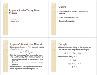
1. Lyapunov Stability Theory: Linear
Systems
M. S. Fadali
Professor of EE
1
Outline
 Lyapunov’s (first, indirect) linearization
method.
 Linear time-invariant case.
 Domain of attraction.
2
Lyapunov’s Linearization Method
 Linearize nonlinear system in vicinity
of equilibrium :
.
 Find the eigenvalues of the linearized system.
The equilibrium of the nonlinear system is:
◦ Exponentially stable if all the eigenvalues are in the
open LHP.
◦ Unstable if one or more of its eigenvalues is in the
open RHP.
◦ Inconclusive for LHP eigenvalues and one or
more eigenvalues on the imaginary axis.
3
Example
 Determine the stability of the equilibrium
of the mechanical system at the origin
 Equilibrium with
4

2. Nonlinear State Equations
 Physical state variables
 State Equations
5
Linearization and Stability
 Equilibrium state
 Linearized model with
 Characteristic polynomial and stability
,
 Stable ,
6
Linear Time-invariant Case
The LTI system
is asymptotically stable if and only if for
any positive definite matrix there exists
a positive definite symmetric solution to
the Lyapunov equation
7
Proof: Sufficiency
 Use a quadratic Lyapunov function
globally exp. stable.
8

3. Proof: Necessity
 Let Hurwitz
→
9
Symmetric Positive Definite
for some nonzero
iff is not an observable pair.
for observable.
Note: can be positive semidefinite.
10
Uniqueness
Subtract
constant if and only if
11
Remarks
 Recall that the original Lyapunov theorem
only gives a sufficient condition.
 If we start with (i.e. with ) and
solve for , the condition the test may or
may not work.
 If we start with (i.e. with the derivative
and we find a the condition is necessary
and sufficient.
12

4. Example
Determine the stability of the system with
state matrix
using the Lyapunov equation with .
Note: The system is clearly stable by
inspection since is in companion form.
13
Solution
14
• Multiply
• Equate to obtain three equations in three unknowns.
Equivalent Linear System
15
Choose
 not positive definite.
 No conclusion: sufficient condition only.
 Choose and solve for .
16

5. MAPLE
Compute:
with(LinearAlgebra):
Transpose(A).P+P.A
Solve the equivalent linear system: M.p=-q
p is a vector whose entries are the entries
of the P matrix, similarly define q
LinearSolve(M,B)
17
Equivalent Linear System
18
MATLAB
 Solve a different equation.
 Identical to our equation with
replaced by .
 Eigenvalues are the same!
19
MATLAB Example
>> A=[0,1;-6,-5];
>> Q=eye(2)
>> P=lyap(A,eye(2))
P =
0.5333 -0.5000
-0.5000 0.7000
>> eig(P)
ans =
0.1098
1.1236
20

6. To Get Earlier Answer
>> P=lyap(A',eye(2))
P =
1.1167 0.0833
0.0833 0.1167
21







1167
.
0
08333
.
0
08333
.
0
1167
.
1
P
Domain (Ball, Region) of Attraction
 Region in which the trajectories of the
system converge to an asymptotically
stable equilibrium point.
 Difficult to estimate, in general.
 Can be estimated using the linearized
system in the vicinity of the asymptotically
stable equilibrium.
22
Example
Equilibrium
Lyapunov function candidate for
23
Calculate
For
24

7. Simulation Results
 The ball of attraction can be estimated
to be
 Although for
we have this
region includes divergent trajectories
because is not an invariant set. For
example, the trajectory starting at
crosses then
diverges.
25
Theorem 3.9
 Equilibrium of
I. compact set containing ,
invariant w.r.t. the solutions of
II.
Then the region of attraction of
26
Proof
 Under the assumptions
 is the largest invariant set in
 By La Salle’s Theorem, every solution
starting in approaches as , i.e.
approaches as
 is an estimate of the domain of
attraction.
27
Example
For
28

8. Invariant Set
Minimum value at edge
29
Estimate Using Linearized system
Solve
30
Example
Equilibrium
Solve
for
31
Contours
32
-3 -2 -1 0 1 2 3
-1.5
-1
-0.5
0
0.5
1
1.5
2