1. January 2016 • Volume 2 • Number 3 9
Experimental Investigation of Wet Gas
Dew Point Pressure Change With Carbon
Dioxide Concentration
U. ODI
ENI Petroleum
H. EL HAJJ
Halliburton Technology Center
Saudi Arabia
A. GUPTA
Aramco Research Center
Houston
Abstract
Dew point pressure is a critical measurement for any wet gas
reservoir. Condensate blockage is likely when the reservoir pres-
sure drops below the dew point pressure, which can result in a re-
duction of gas productivity. One possible treatment fluid—carbon
dioxide—has the ability to lower dew point pressure, and thus
delay the onset of condensate blockage. Errors in measuring dew
point pressure can lead to errors in the estimation of the onset
of condensate blockage and be detrimental to the management
of wet gas fields. This work presents experimental verification
of a new method of determining dew point pressure for wet gas
fluids. This method was applied to determine the experimental
dew point pressure of several wet gas mixtures as a function of
carbon dioxide concentration. Results obtained from this method
are compared to calculated values based on the Peng Robinson
equation of state. Experimental results also support the general
observation that carbon dioxide has the ability to lower the dew
point pressure of wet gas fields.
The results of this work are applicable to Enhanced Oil/Gas
Recovery processes that utilize carbon dioxide and for the CO2
Huff and Puff process that uses carbon dioxide to remove and
prevent further build-up of condensate banks around wells in wet
gas reservoirs. This work investigates experimental conditions
showing the change in dew point pressure as a function of carbon
dioxide concentration. This dynamic relationship can be used to
tune equation of state models which, in turn, allows more accu-
rate reservoir modelling of the hydrocarbon recovery process.
Introduction
Condensation is a critical factor in determining the perfor-
mance of wet gas fields. Condensation in the near wellbore region
can lead to a dramatic reduction in gas flow due to the reduction
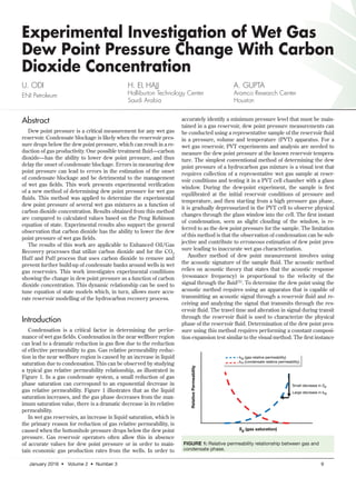
of effective permeability to gas. Gas relative permeability reduc-
tion in the near wellbore region is caused by an increase in liquid
saturation due to condensation. This can be observed by studying
a typical gas relative permeability relationship, as illustrated in
Figure 1. In a gas condensate system, a small reduction of gas
phase saturation can correspond to an exponential decrease in
gas relative permeability. Figure 1 illustrates that as the liquid
saturation increases, and the gas phase decreases from the max-
imum saturation value, there is a dramatic decrease in its relative
permeability.
In wet gas reservoirs, an increase in liquid saturation, which is
the primary reason for reduction of gas relative permeability, is
caused when the bottomhole pressure drops below the dew point
pressure. Gas reservoir operators often allow this in absence
of accurate values for dew point pressure or in order to main-
tain economic gas production rates from the wells. In order to
accurately identify a minimum pressure level that must be main-
tained in a gas reservoir, dew point pressure measurements can
be conducted using a representative sample of the reservoir fluid
in a pressure, volume and temperature (PVT) apparatus. For a
wet gas reservoir, PVT experiments and analysis are needed to
measure the dew point pressure at the known reservoir tempera-
ture. The simplest conventional method of determining the dew
point pressure of a hydrocarbon gas mixture is a visual test that
requires collection of a representative wet gas sample at reser-
voir conditions and testing it in a PVT cell chamber with a glass
window. During the dew-point experiment, the sample is first
equilibrated at the initial reservoir conditions of pressure and
temperature, and then starting from a high pressure gas phase,
it is gradually depressurized in the PVT cell to observe physical
changes through the glass window into the cell. The first instant
of condensation, seen as slight clouding of the window, is re-
ferred to as the dew point pressure for the sample. The limitation
of this method is that the observation of condensation can be sub-
jective and contribute to erroneous estimation of dew point pres-
sure leading to inaccurate wet gas characterization.
Another method of dew point measurement involves using
the acoustic signature of the sample fluid. The acoustic method
relies on acoustic theory that states that the acoustic response
(resonance frequency) is proportional to the velocity of the
signal through the fluid(1). To determine the dew point using the
acoustic method requires using an apparatus that is capable of
transmitting an acoustic signal through a reservoir fluid and re-
ceiving and analyzing the signal that transmits through the res-
ervoir fluid. The travel time and alteration in signal during transit
through the reservoir fluid is used to characterize the physical
phase of the reservoir fluid. Determination of the dew point pres-
sure using this method requires performing a constant composi-
tion expansion test similar to the visual method. The first instance
FIGURE 1: Relative permeability relationship between gas and
condensate phase.
RelativePermeability
Sg (gas saturation)
Small decrease in Sg
Large decrease in krg
krg (gas relative permeability)
kro (condensate relative permeability)

2. 10 www.ceti-mag.ca
CANADIAN ENERGY TECHNOLOGY & INNOVATION
When analyzing the results of the constant composition expan-
sion (CCE) experiment—a general test used to estimate bubble
and dew points using the visual method—it is important to un-
derstand the thermodynamic changes that occur to the reservoir
fluid during phase change. Determination of bubble points using
the graphical method based on CCE tests is made possible by the
large differences between the isothermal compressibility of the
liquid phase less the dense gas phase.
Determination of phase changes involved in the transition from
the gas phase to the liquid phase is much more difficult due to in-
distinguishable slope changes. Such is the case when looking at
dew points of gas condensates. This can be illustrated by con-
sidering an isotherm in the pressure and temperature phase dia-
gram of an example wet gas/condensate as illustrated by Figure
2. Starting from the super critical gas region, as the pressure
drops isothermally, there is an expansion of the system volume as
the wet gas/condensate transitions from the supercritical gas re-
gion to the gas region and finally past the dew line. When the res-
ervoir fluid undergoes decompression, there is a gradual change
in the total isothermal compressibility of the reservoir fluid. This
can be understood by considering the total isothermal compress-
ibility of the reservoir fluid inside the PVT cell, which can be de-
scribed by the following equation.
= −
∂
∂





c
V
V
p
1
T
t
t
........................................................................................(1)
Where cT is the total isothermal compressibility, Vt is the total
volume of the fluid mixture in the PVT cell, and p is the pres-
sure of the fluid. The partial derivative, Vt/p, is at isothermal
conditions. Above the dew point line, the total isothermal com-
pressibility represents the isothermal compressibility of the su-
percritical gas phase. Below the dew point, the total isothermal
compressibility can be derived using material balance between
the gas and liquid phases (see Appendix). The final derived form
of the total isothermal compressibility for all stages of isothermal
compression is represented in the following expression for the
PVT cell.
= + +
ρ
−
ρ






∂
∂





c c f c f
V
m
p
1 1 1
T G G L L
t L G
G
................................................(2)
Where cG is the gas compressibility, fG is the gas saturation in the
PVT cell, cL is the liquid compressibility, fL is the liquid saturation
in the PVT cell, ρL is liquid density in the PVT cell, ρG is the gas
density in the PVT cell, and mG is the mass of the gas phase of
the PVT cell. The partial derivative, mG/p, is at isothermal con-
ditions. In addition, fG + fL = 1 is valid because of material balance
within the PVT cell. The total isothermal compressibility expres-
sion has important implications at saturation pressures and in the
two-phase region.
For example, consider black oil bubble points. Above the
bubble point pressure, black oils have small, approximately con-
stant compressibility(3). At and below the bubble point, the black
oil exhibits large increases in total isothermal compressibility.
This is because the gas released from the black oil at or below the
bubble point is extremely compressible. Additionally, gas density
is generally smaller than liquid density. Combining these obser-
vations with the fact that black oil CCEs have a negative mG/p
for changes in pressure, it is evident that at the bubble point
black oils experience sharp increases in total isothermal com-
pressibility as illustrated in Figure 3. This increase is caused by
the product of the (1/ρL-1/ρG) which is negative and the mG/p
of a liquid signature in the vibrational response during this test is
defined as the dew point pressure. The limitation of this method
is that it still requires the visual method to validate the estimated
dew point. Thus, any PVT apparatus that is designed to imple-
ment the acoustic method must have a window cell to ensure
accuracy, in addition to the equipment that can transmit and re-
ceive the acoustic signal. The capital investment needed for the
acoustic method can be significantly higher than for the standard
PVT cell used for the visual method.
Potsch et al.(2) presented a method to determine the dew point
pressure graphically. Their method involved using the real gas
equation of state to calculate the total moles in the reservoir fluid
sample for several measurements of pressure above the dew
point pressure. They proposed that below the dew point pres-
sure, condensation will cause calculated moles in the gas phase
to be different from the actual number of moles. They proposed
that the first instance from the deviation from the true amount of
moles indicates dew point pressure. Their work may be in error
because the real gas equation of state is not valid for fluids near
saturation pressure, as indicated by their plots of the calculated
molar quantity changing with pressure above dew point pressure.
For a valid method, the calculated amount of moles would have
remained constant because of the conservation of mass in the
PVT cell (no mass exits or leaves the PVT cell). Potsch et al.’s at-
tempt to characterize the dew point pressure appears to be theo-
retically inaccurate.
The method proposed in this paper is based on tracking
changes in isothermal compressibility to pinpoint dew point pres-
sure measurements in wet gas fluid samples. Using this method,
this work demonstrates the potential of using CO2 to lower the
dew point pressure as a solution to condensate blockage. Com-
parisons with Peng Robinson equation of state are used to vali-
date the approach illustrated in this work.
Saturation Pressure Theory
Dew point pressure can be described as the pressure at which
a gas starts condensing into a liquid phase. Pressure and tem-
perature phase diagrams are generally used to describe bubble
points and dew points as functions of pressure and temperature.
For example, Figure 2 illustrates a pressure and temperature
phase diagram for a wet gas. The dew-point line (the line that is to
the right of the critical point in Figure 2) can be used to describe
variation of dew point pressure with temperatures.
0
5,000
10,000
15,000
20,000
25,000
30,000
35,000
40,000
100 200 300 400 500 600
Pressure(kPa)
Temperature (K)
366 K (200˚F) CCE
Critical Point
Liquid
Phase
Bubble Line Dew Line
Gas & Liquid
Phases
Gas Phase
Supercritical Gas Phase
CCE
Isotherm
FIGURE 2: Pressure and temperature diagram for wet gas/
condensate with cce isotherm going from the supercritical gas
phase region to the two-phase gas and liquid region.

3. January 2016 • Volume 2 • Number 3 11
CANADIAN ENERGY TECHNOLOGY & INNOVATION
term, which is also negative (caused by the increased gas mass
for decreasing pressures associated with typical black oils).
The behaviour of a condensate contrasts from a black oil. At
above the dew point the condensate exists as a supercritical fluid.
At and below the dew point pressure the supercritical portion par-
titions into a wet gas with some liquid dropout. This gas below
the dew point pressure has an isothermal compressibility slightly
larger than the supercritical fluid. In addition, the liquid conden-
sate that drops out of the wet gas exhibits initial large increases of
liquid saturation at the dew point, followed by decrease in liquid
saturation as the pressure decreases below the upper dew point.
This observation can be seen in Figure 4 for the sample wet gas.
The liquid saturation decreases because lighter components
vapourize out of the liquid phase leaving heavier components be-
hind to make up the majority of the liquid phase. The evidence is
seen in Figure 5, which indicates an increase in liquid density as
the pressure drops.
For gas condensates, the liquid density increases corre-
sponding to the liquid phase becoming richer in heaver com-
ponents. Figure 5 illustrates a negative ρ/p relationship. A
consequence of this is that the liquid isothermal compressibility,
represented by cL = (1/p)*ρ/p, results in a negative value. For
gas condensates, these liquid compressibilities are necessary in
maintaining the material balance detailed in the total isothermal
compressibility equation. This material balance is essential be-
cause it is one of the reasons why total isothermal compress-
ibility does not change sharply. Combining this observation with
the fact that gas condensate CCEs have a positive ∂mG/∂p as
the pressure reduces towards the dew point, it is evident that at
the dew point pressure gas condensates experience gradual in-
creases in total compressibility (when compared to black oils).
This speed of increase in total compressibility is less than for the
black oil because of the product of (1/ρL – 1/ρG) which is nega-
tive and the mG/p term which is positive (caused by the de-
creased gas mass for decreasing pressures at the dew point).
Therefore, the product, (1/ρL – 1/ρG)* mG/p is negative at the
dew point and thus is one of the factors that reduces the inflection
seen in the total isothermal compressibility plot. To illustrate this,
the simulated gas isothermal compressibility and total isothermal
compressibility for the sample wet gas are illustrated in Figure 6.
It can be seen that the total and gas isothermal compressibil-
ities track one another below the dew point (34,600 kPa) and
eventually deviate from one another at pressures less than the
dew point. At the dew point, the gas isothermal compressibility
is slightly larger than the total isothermal compressibility. This
difference occurs because of the negative product (1/ρL – 1/ρG)*
mG/p and the negative oil isothermal compressibility which are
a result of the retrograde behaviour of the gas condensate. In ad-
dition to this, the impact of the oil isothermal compressibility is
tempered by the low oil volume fraction at the dew point pres-
sure. Similarly, the impact of the 1/ρL – 1/ρG)* mG/p term is
tempered by the total volume (i.e., the 1/Vt factor). A summary of
the impact of each term is listed in Table 1.
Determining the increase in the total isothermal compress-
ibility with pressure is the main premise of the method used in
this work. For both black oils and gas condensates the total iso-
thermal compressibility increases at the saturation point. It can
be seen that before the saturation pressure, the total isothermal
0.000001
0.00001
30,000 35,000 40,000 45,000 50,000
IsothermalCompressibility(1/kPa)
Pressure (kPa)
FIGURE 3: CCE of example 34.9 API black oil at 400 K (bubble
point at 33,500 psia) that illustrates sharp compressibility contrast
at the bubble point.
0
0.05
0.1
0.15
0.2
0.25
0.3
0 10,000 20,000 30,000 40,000 50,000
LiquidSaturation
Pressure (kPa)
FIGURE 4: Liquid saturation for wet gas/condensate system during
CCE at 366 K (retrograde behavior).
0
100
200
300
400
500
600
700
800
900
0 10,000 20,000 30,000 40,000 50,000
Density(kg/m3)
Pressure (kPa)
Liquid Gas
FIGURE 5: Density for wet gas/condensate system during CCE at
366 K.
0.000001
0.00001
0.0001
0.001
0.01
0 10,000 20,000 30,000 40,000 50,000
IsothermalCompressibility(1/kPa)
Pressure (kPa)
Total Gas
FIGURE 6: Comparison between total compressibility and gas
compressibility of wet gas sample at 366 K.

4. 12 www.ceti-mag.ca
CANADIAN ENERGY TECHNOLOGY & INNOVATION
same analysis is applied to experimental wet gas/condensate
fluids.
Experimental Design
To test the new dew point determination method several con-
densate mixtures were created. These condensate mixtures in-
clude a base condensate mixture with a 1% molar composition
of CO2. The other condensate mixtures contained 10% and 15%
molar concentrations of CO2. The base condensate mixture com-
ponents can be seen in Table 2. Critical properties were based on
values reported in literature. Acentric factor values were obtained
from Winnick(4) and Poling et al.(5). Density values were obtained
from the API data book. The purpose of using these condensate
mixtures was to understand the effect of adding CO2 to the base
concentration and to also illustrate the methodology of the new
dew point determination method.
To load, mix, and observe the hydrocarbon phase transitions
of the proposed condensate mixtures, a pressure, volume and
temperature (PVT) system (illustrated in Figure 8) was used. As
an example of the process used to create and transfer a mixed
condensate, consider the base condensate in Table 2. To calcu-
late the necessary molar amounts of each component requires
determination of the volumetric amount of each component at
ambient conditions. At atmospheric pressure and room tempera-
ture the only components that are in the liquid phase are octane
compressibility is linear with respect to pressure on a semi log
plot. An example of this is illustrated in Figure 7 for a wet gas.
When the total isothermal compressibility deviates from the
linear isothermal compressibility behaviour during the CCE pro-
cess, it is theorized that this is the dew point pressure. The gen-
eral procedure to use isothermal compressibility for determining
saturation points involves completing the following tasks.
1. Use the CCE experimental data (pressure and volume data)
to calculate the central difference approximation of the iso-
thermal compressibility as indicted in Equation (1).
2. Create a plot of the calculated isothermal compressibility
versus the experimental pressure of the CCE experiment.
3. Starting from the highest pressure of the isothermal com-
pressibility versus pressure plot, locate the first linear line
and draw a line through it.
4. Find the nearest linear line next to the first linear line and
draw a line through it.
5. The intersection between the first and second linear line is
the observed saturation point (dew point for gas conden-
sates; bubble point for black oils).
As an example of this novel analysis, consider the typical wet
gas/condensate system. Its total isothermal compressibility plot
can be seen in Figure 7. Using the previously described com-
pressibility analysis, it can be seen that the dew point of this fluid
at 366 K is 34,500 kPa which matches with the Peng Robinson ap-
proximation of 34,600 kPa.
This example was based on a Peng Robinson equation of state
of the example wet gas/condensate fluid described earlier. This
TABLE 1: Total isothermal compressibility components at saturation pressures (sign change and total isothermal compressibility
response).
m
p
1 1
L G
G
ρ
−
ρ






∂
∂





 Total
cGfG cLfL Compressibility Response
Bubble Point “positive” “positive” “positive” Sharp Increase
Dew Point “positive” “negative” “negative” Gradual Increase
0.000001
0.00001
0.0001
0.001
0.01
0 10,000 20,000 30,000 40,000 50,000
IsothermalCompressibility(1/kPa)
Pressure (kPa)
1st linear line
2nd linear line
Dew Point
Pressure =
34,500 kPa
0.000001
0.00001
0.0001
0.001
0.01
0 10,000 20,000 30,000 40,000 50,000
IsothermalCompressibility(1/kPa)
Pressure (kPa)
FIGURE 7: Wet gas/condensate sample dew point determination at 366 K: a) isothermal compressibility before analysis; b) isothermal
compressibility after analysis.
a) b)
TABLE 2: Base composition for experimental studies.
Composition Molecular Critical Temperature Critical Pressure Acentric Liquid Density at
Component (mol %) Weight (˚K) (kPa) Factor [289 K (60˚F), kg/m3]
Methane 83 16.04 191 4,600 0.007 300
Carbon Dioxide 1 44.01 304 7,370 0.225 817
Ethane 4 30.07 305 4,870 0.099 356
Propane 3 44.1 370 4,250 0.153 507
Octane 3 114.23 580 2,920 0.398 706
Dodecane 6 170.34 675 2,170 0.576 752

5. January 2016 • Volume 2 • Number 3 13
CANADIAN ENERGY TECHNOLOGY & INNOVATION
and dodecane. The volumetric amount of these liquid compo-
nents can be found by using the following equation.
=
ρ
V
MW y n
i
i i t
i
.........................................................................................(3)
Where Vi is the ith liquid component’s feed liquid volume, ρi is the
ith liquid component’s density at standard conditions, MWi is the
ith liquid component’s molecular weight, and yi is the ith compo-
nent’s mole fraction in the gas condensate mixture.
The remaining components in the condensate mixture are
gases at standard conditions. To feed the required number of
moles of each gas component into the PVT system requires
loading the gas components at a target pressure and corre-
sponding volume. Setting the volume of each gas is much easier
to control than pressure, therefore the loading pressure of each
gas component was determined using the Virial equation of state.
The following steps can be used to determine the feed pressure
of a component using the Virial equation of state.
1. Guess a working pressure of the component, Pi, and loading
volume of the component, Vi.
2. For the component, determine the reduced pressure, Pr,
and reduced temperature, Tr.
=T
T
Tr
c
....................................................................................................(4)
=P
P
Pr
c
...................................................................................................(5)
Where Tc and Pc are the critical temperature and critical
pressure of the component.
3. Calculate the Virial coefficients(4) using the following
equations.
= − −
B T0.083 0.422 r
(0) 1.6
.......................................................................(6)
= − −
B T0.139 0.172 r
(1) 4.2
........................................................................(7)
= +ωB B Br
(0) (1)
.....................................................................................(8)
Where ω is the acentric factor of the component.
4. Calculate the compressibility factor of the component, zi.
= +z
B P
T
1i
r r
r
............................................................................................(9)
5. Recalculate the working pressure, Pi, using the gas law.
=P
z y n RT
Vi
i i t
i
.......................................................................................(10)
6. Repeat steps 2 – 5 using the calculated Pi from step 5. Iterate
until the value of Pi converges.
The procedure to calculate the feed pressure of each compo-
nent is based on the Virial equation state and assumes that the
reduced pressure and reduced temperature are within the low
density region. This region corresponds to a reduced tempera-
ture and reduced pressure relationship that results in reduced
temperatures greater than approximately Tr = 0.436Pr + 0.6(4).
Once the feed liquid quantities and feed gas components are
calculated it is important to ensure that the total mixture can reach
system pressures larger than the expected dew point pressure of
the condensate system. This is important because the CCE ex-
periments are begun at pressures much larger than the dew point
pressure. Using this assumption, values of the compressibility
factor were calculated using an empirical version of the standing
correlation described by Cronquist(6) which is dependent on the
pseudo critical properties of the mixed condensate. The pseudo
critical temperature and pressure were calculated using a correla-
tion by Piper et al(7) which accounts for reservoir impurities such
as nitrogen, hydrogen sulfide and carbon dioxide. As an example
FIGURE 8: PVT System for dew point measurement: a) oven; b) computer gathering equipment; c) top pump B; d) PVT visual cell; e) bottom
pump A.

6. 14 www.ceti-mag.ca
CANADIAN ENERGY TECHNOLOGY & INNOVATION
of this process, consider the base condensate listed in Table 2.
The phase diagram of this condensate is illustrated in Figure 9.
From the phase diagram, it can be seen that for a CCE experi-
ment at 366 K, the dew point pressure is approximately 34,500
kPa. Therefore, at 366 K the initial pressure of the system is set to
41,400 kPa, which is greater than the dew point pressure. Using
this and the volume of the PVT cell it is possible to calculate the
total amount of moles that will ensure that the PVT cell reaches
the initial starting pressure. These steps are listed here.
1. Calculate the gas specific gravity, γg, of the gas condensate
sample.
∑
γ =
y MW
29g
i i
i
6
.....................................................................................(11)
2. Calculate the pseudo critical temperature, Tpc, and pseudo
critical pressure, Ppc, using Piper et al.(7) correlation. As-
sume a pressure larger than the dew point pressure, Pt, and
a temperature, Tt, used for the CCE experiments.
∑= η + η





 +η γ + η γ
=
J y
T
Pf
f
f
c
c f
g g0
1
3
4 5
2
................................................(12)
∑= β + β








+β γ +β γ
=
K y
T
P
f
f
f
c
c f
g g0
1
3
4 5
2
.............................................(13)
=T
K
Jpc
2
..............................................................................................(14)
=P
T
Jpc
pc
..............................................................................................(15)
The parameter, f, corresponds to the reservoir fluid impuri-
ties in the following order H2S, CO2 and N2. Values for ηf and
βf are shown in Table 3.
3. Calculate the compressibility factor, zt, of the condensate
sample at the expected experimental conditions above the
dew point pressure using the Standing correlation(6).
=T
T
Tpr
t
pc
..............................................................................................(16)
=P
P
Ppr
t
pc
..............................................................................................(17)
( )= − − −A T T1.39 0.92 0.36 0.101pr pr
0.5
..............................................(18)
( )
( )
= − +
−
−








+
−
B T P
T
P
P
T
0.62 0.23
0.066
0.86
0.037
0.32
10 1
pr pr
pr
pr
pr
pr
2
6
9
........(19)
= −C T0.132 0.32log pr
.........................................................................(20)
=
( )− − +
D 10
T T0.3106 0.49 0.1824pr pr
2
..............................................................(21)
( )= + − +z A A e CP1t
B
pr
D
....................................................................(22)
4. Recalculate the pressure of the cell at the CCE conditions
using the expanded volume of the cell, Vt, and the gas law.
=P
z n RT
Vt
t t t
t
..........................................................................................(23)
5. Repeat steps 3 – 4 using the calculated Pt from step 4. Keep
doing this until the difference between each iterative Pt is
minimized.
The preceding procedure is dependent on the total amount of
moles, nt, in the PVT cell which is also a necessary component
in the calculation of the volumetric amount of liquid needed and
the calculation of the loading pressure for the gas components.
0
5,000
10,000
15,000
20,000
25,000
30,000
35,000
40,000
45,000
100 200 300 400 500 600
Pressure(kPa)
Temperature (K)
FIGURE 9: Pressure-temperature phase diagram for base
condensate.
TABLE 3: Piper et al.(7) parameters for pseudo critical temperature
pressure calculation.
f ηf βf
0 0.11582 3.8216
1 -0.45820 -0.065340
2 -0.90348 -0.42113
3 -0.66026 -0.91249
4 0.70729 17.438
5 -0.099397 -3.2191
TABLE 4: Calculated Liquid Volumes for Base Case
Component Feed State Vi, cm3
Methane gas n/a
Carbon Dioxide gas n/a
Ethane gas n/a
Propane gas n/a
Octane liquid 6.64
Dodecane liquid 18.6

7. January 2016 • Volume 2 • Number 3 15
CANADIAN ENERGY TECHNOLOGY & INNOVATION
Therefore, any changes made to the total amount of moles in the
preceding procedure have to be followed by recalculations of
liquid volumes and gas component loading pressures (at specified
loading volumes). As example of these considerations, consider
the base condensate mixture in Table 2. For a CCE experiment at
366 K for a PVT cell with 18 cm3 volume (with a value of 100 cm3
out of a possible 200 cm3 of additional adjustable volume used for
compression and expansion) the calculation of the necessary pa-
rameters are listed in Tables 4 and 5.
The Peng Robinson equation of state was used to check the ac-
curacy of the loading pressure calculation. This was done by es-
timating the loading volume using the Peng Robinson equation
of state. Then, by using the molar amounts of the gaseous com-
ponent, the calculated loading pressure from Table 5, and a feed
temperature of 294 K. The Peng Robinson check is illustrated in
Table 6 and shows approximate agreement with the Virial equa-
tion of state.
The total amount of moles needed to bring the system to 41,400
kPa was found to be 1.4 moles. This quantity is verified because
it can be used to calculate the 41,400 kPa desired pressure at 366
K and 118 cm3 of available volume (Table 7). This quantity is also
verified by the Peng Robinson equation of state that determined
that the molar volume of the experimental wet gas fluid was 77.4
cm3/mol. This corresponds to a Peng Robinson estimate of 1.5
moles, which is comparable to the amount determined using the
Standing correlation. This quantity was also found to satisfy the
procedure of determining the gas loading pressures (Table 5)
and the required liquid volumes (Table 4).
Experimental Results
Dew points were determined for the synthetically designed
condensate mixtures by observing changes in compressibility
from constant composition expansion experiments and verified
by equation of state models such as the Peng Robinson equation
of state. As an example of the process of using the isothermal
compressibility to determine the dew point pressure, consider
the 15% CO2 case at 366 K. Its CCE isotherm (Figure 10) illus-
trates the pressure volume relationship for this fluid. The total
isothermal compressibility of this fluid was calculated for each
pressure point (Figure 11) using a central finite difference ver-
sion of Equation (1).
Figure 11 illustrates a substantial increase in the isothermal
compressibility at approximately 29,000 kPa. This large increase
is attributed to the first instance of liquid saturation in the PVT
cell. According to Equation (2), the mass transfer from the gas
phase to the liquid phase can cause substantial increases in
the total isothermal compressibility. Using this large rise in
TABLE 5: Gas calculations for loading pressures, Pi, using specified loading volumes, Vi, for base case.
Feed Pi guess Vi Pi calculated
Component State (kPa) Tr Pr B(0) B(1) Br zi (cm3) (kPa)
Methane gas 18,600 1.55 0.718 -0.13 0.111 -0.13 0.669 100 18,600
Carbon Dioxide gas 331 0.968 0.144 -0.36 -0.0580 -0.37 0.983 100 331
Ethane gas 1210 0.964 0.202 -0.36 -0.0613 -0.37 0.904 100 1,210
Propane gas 862 0.796 0.124 -0.52 -0.309 -0.57 0.855 100 862
Octane liquid n/a n/a n/a n/a n/a n/a n/a n/a n/a
Dodecane liquid n/a n/a n/a n/a n/a n/a n/a n/a n/a
TABLE 6: Loading pressure by comparing virial equation of state
and calculated volume vs. volume calculated from Peng Robinson
equation of state.
Vi Peng
Molar Pi Robinson
Feed Vi Amount Calculated Estimate
Component State (cm3) (moles) (kPa) (cm3)
Methane gas 100 1.14 18,600 118
Carbon Dioxide gas 100 0.0137 331 99
Ethane gas 100 0.0548 1,210 98
Propane gas 100 0.0411 862 97
Octane liquid n/a n/a n/a n/a
Dodecane liquid n/a n/a n/a n/a
TABLE 7: Parameters used to calculate 1.4 total moles needed to
reach 41,400 kPa at 366 K (Volume used for calculation is
118 cm3).
γg 1.03
J 0.736
K 18.3
Tpc (K) 254
Ppc (kPa) 4,280
Tpr 1.16
Ppr 9.67
A 0.163
B 20.5
C 0.111
D 0.972
zt 1.17
Pt (kPa) 41,400
FIGURE 10: CCE isotherm for 15% CO2 in base case at 366 K.
0
5,000
10,000
15,000
20,000
25,000
30,000
35,000
40,000
45,000
50 60 70 80 90 100 110
Pressure(kPa)
Volume (cm3)
15% CO2 in Base: Pressure vs. Volume at 366˚K
FIGURE 11: Dew points determination using isothermal
compressibility vs. pressure plot for 15% CO2 in base case at 366 K.
0.000001
0.00001
0.0001
0.001
0 10,000 20,000 30,000 40,000 50,000
IsothermalCompressibility(1/kPa)
Pressure (kPa)
15% CO2 in Base: Isothermal
Compressibility vs. Pressure at 366 K
Dew Point Pressure = 29,000 kPa

8. 16 www.ceti-mag.ca
CANADIAN ENERGY TECHNOLOGY & INNOVATION
isothermal compressibility, the dew point for the 15% CO2 case is
approximately 29,000 kPa.
The isothermal compressibility methodology was applied to
the base case, 10% CO2 case and the 15% CO2 case. Results of
the dew point measurement of each case can be seen in Table 8
and Figure 12. Plots of the matched experimental data for each
case superimposed on the Peng Robinson theoretical data and
the ideal gas approximation are shown in Figure 13.
When comparing the theoretical dew point pressure among
each case at 366 K it can be seen that CO2 has the unique ability
in reducing the dew point pressures. The experimental results
show some deviation from the theoretical observation. This error
is attributed to preparing the wet gas samples and running the
experiments in a high pressure environment. Minute leaks can
occur in high pressure environments. The possibility of these
minute leaks are an inescapable obstacle in running these experi-
ments. Nonetheless, it is observed that CO2 theoretically reduces
the dew point pressure of wet gas/condensate fluids as is veri-
fied by the Peng Robinson equation of state. This is observed in
Figure 12 and Figure 14, which is a plot of the relative volume
(PVT volume divided by the volume at the dew point).
The relative volume plot in Figure 14 indicates that CO2 de-
creases the corresponding pressures observed during CCE. In
addition to this, the overall phase diagram of the gas condensate
illustrates that the phase envelope decreases as a function of CO2
concentration. This is conveyed in Figure 15. These results can
be explained by analyzing previous studies of CO2 with hydro-
carbon systems. Monger et al.(8) were able to illustrate in their
Appalachian crude oil system that the crude oil aromaticity cor-
related with improved hydrocarbon extraction into a CO2 rich
TABLE 8: Comparison of dew point pressure measurements at
366 K.
Theoretical % absolute
Experimental (Peng Robinson) Error
Base Case 38,800 kPa 34,600 kPa 12
10% CO2 in Base 25,500 kPa 32,000 kPa 20
15% CO2 in Base 29,000 kPa 30,600 kPa 5
a)
0.000001
0.00001
0.0001
0.001
10,000 20,000 30,000 40,000 50,000
IsothermalCompressibility(1/kPa)
Pressure (kPa)
Base Composition
Dew Point Pressure = 38,800 kPa
PengRobinson Experimental Ideal Gas
0.000001
0.00001
0.0001
0.001
0.01
0 10,000 20,000 30,000 40,000 50,000
IsothermalCompressibility(1/kPa) Pressure (kPa)
10% CO2 Composition
Dew Point Pressure = 25,500 kPa
PengRobinson Experimental Ideal Gas
0.000001
0.00001
0.0001
0.001
0 10,000 20,000 30,000 40,000 50,000
IsothermalCompressibility(1/kPa)
Pressure (kPa)
15% CO2 Composition
Dew Point Pressure = 29,000 kPa
PengRobinson
Experimental
Ideal Gas
FIGURE 13: Match experimental data and theoretical data
comparison: a) base case; b) 10% CO2 in base; c) 15% CO2 in
base.
b)
c)
0.000001
0.00001
0.0001
0.001
0.01
0 10,000 20,000 30,000 40,000 50,000
IsothermalCompressibility(1/kPa)
Pressure (kPa)
Base Dew Point = 34,600 kPa
10% CO2 in Base Dew Point = 32,000 kPa
15% CO2 in Base Dew Point = 30,600 kPa
Base 10% CO2 in Base 15% CO2 in Base
2,000
7,000
12,000
17,000
22,000
27,000
32,000
37,000
42,000
0 2 4 6 8 10 12 14 16
Pressure(kPa)
CO2 mol%
Theoretical (Peng Robinson)
Experimental
FIGURE 12: Dew point comparison as function of CO2
concentration in base composition at 366˚K: a) experimental vs.
theoretical comparison; b) theoretical compressibility indicating dew
point pressures.
a)
b)
12,000
17,000
22,000
27,000
32,000
37,000
42,000
47,000
52,000
0.6 0.8 1 1.2 1.4 1.6 1.8 2 2.2
Pressure(kPa)
Relative Volume
Base
10% CO2 in Base
15% CO2 in Base
FIGURE 14: Theoretical relative volume of base condensate as
function of CO2 at 366 K.

9. January 2016 • Volume 2 • Number 3 17
CANADIAN ENERGY TECHNOLOGY & INNOVATION
phase. In addition to this, Monger et al. observed that CO2 has
the ability to lower miscible pressures for paraffin fluids that do
not contain large amounts of aromatic content. In terms of gas
condensate systems, this means that CO2 forces the lighter end
hydrocarbons into the CO2 rich phase. This is beneficial because
the CO2 rich phase is a supercritical gas in typical reservoir con-
ditions, implying that CO2 is lowering the hydrocarbon’s dew
point pressure.
In terms of liquid compressibility, the Peng Robinson approxi-
mation of the liquid saturation during CCE (Figure 16) gives an in-
dication that there is less liquid dropout occurring as the amount
of CO2 increases. With regard to production from gas condensate
reservoirs, this is beneficial because it shows that increasing the
CO2 concentration can decrease the maximum amount of liquid
saturation that can occur in the reservoir.
Thermodynamic Justification of Using CO2
CO2 injection into condensate banks has a theoretical justifica-
tion. Consider a wet gas above the dew point and a wet gas below
the dew point. Gibbs free energy is a thermodynamic property
that describes thermodynamic equilibrium. For a mixture, the
change in Gibbs free energy is as follows(4):
∑= − + + µdG SdT Vdp dni i
i ..................................................................(24)
Where G is the Gibbs free energy, S is the entropy, V is the
volume, T is the temperature, n is moles, µi is the chemical po-
tential of component i. The chemical potential of component i is
the rate of change of Gibbs free energy when moles are added at
constant T and P at its current phase. At equilibrium between the
liquid (subscript l) and vapour (subscript v) phases the change in
Gibbs free energies are equal.
∑ ∑− + + µ








= − + + µ








SdT Vdp dn SdT Vdp dni i
i l
i i
i v ............................(25)
In addition to this the chemical potentials of each component
in the mixture are equal at equilibrium and the transport of each
species is equal therefore the expression can be reduced further.
− +  = − + SdT Vdp SdT Vdp
l v
............................................................(26)
( ) ( )− = −V V dp S S dTl v l v
.....................................................................(27)
=
dp
dT
dS
dV ..............................................................................................(28)
From the previous expression the right side’s numerator and
denominator can be divided by the total number of moles, n, of
the system. This leaves the expression to be a function of molar
entropy, s, and molar volume, v.
=
∆
∆
=
∆
∆
dp
dT
S
n
V
n
s
v
....................................................................................(29)
The previous expression can be reduced to a useful form by
using the definition of Gibbs free energy which is the expression,
∆g = ∆h – T∆s, where ∆h is the change in enthalpy. At equilibrium
the difference in free energy between the two phases is 0 there-
fore the change in molar entropy of the system is ∆s = ∆h/T. This
reduces the previous expression into the following form.
=
∆
∆
dp
dT
h
T v ............................................................................................(30)
0
0.05
0.1
0.15
0.2
0.25
0.3
0 10,000 20,000 30,000 40,000 50,000
LiquidSaturation
Pressure (kPa)
Base
10% CO2 in Base
15% CO2 in Base
FIGURE 16: Peng Robinson liquid saturation of base condensate as
function of CO2 at 366 K.
0
5,000
10,000
15,000
20,000
25,000
30,000
35,000
40,000
0 100 200 300 400 500 600
Pressure(kPa)
Temperature (K)
0
10
20
30
40
50
CO2 mol%
Critical
Point
366 K isotherm
0
5,000
10,000
15,000
20,000
25,000
30,000
35,000
40,000
0 20 40 60 80 100
Pressure(kPa)
mol % CO2
FIGURE 15: Peng Robinson phase envelope of gas condensate as function of CO2 concentration: a) pressure temperature phase envelope;
b) pressure composition phase envelope at 366 K.
a) b)

10. 18 www.ceti-mag.ca
CANADIAN ENERGY TECHNOLOGY & INNOVATION
The previous expression is the Clausius-Clapeyron rela-
tionship(4). Solving for the enthalpy term leaves the following
expression.
∆ = −h RT Plncondensation dew ....................................................................(31)
Where Pdew is the dew point of the wet gas and ∆hcondensation is the
heat of enthalpy due to condensation.
The impact of the heat of condensation expression can be un-
derstood by considering a reservoir fluid that has been studied in
literature. This fluid description can be seen in Table 9.
Adding CO2 to this wet gas shrinks the phase envelope and
thus the dew point pressure for a corresponding reservoir tem-
perature as indicated by Figure 17.
The dew point pressure (Table 10) of each phase envelope
(shown by Figure 17) can be obtained using the Peng Robinson
equation of state. From there, the enthalpy of condensation can
be calculated. The enthalpy of condensation is illustrated in
Figure 18.
The heat of condensation is a measure of the heat released
in bringing a fluid from the gas phase to the liquid phase. An
increase in the enthalpy of condensation corresponds to a gas
having difficulty in condensing to a liquid. In the context of CO2’s
interaction with wet gases, the increase in CO2 concentration re-
sults in wet gas fluid having a greater difficulty of having liquid
dropout. This concept is illustrated in Figure 18 and is the ther-
modynamic justification of injecting CO2 to remove condensate
blocking and for CO2 Enhanced Gas Recovery.
TABLE 9: Wet gas composition for compositional simulation(9).
zi Molecular Tc Pc Accentric Tb Zc
Component (%mol) Weight (˚K) (kPa) Factor Vshift (˚K) SG (Visc) Pchor
N2 3.349 28.01 126 3,398 0.037 0.0009 77 0.2724 0.2918 59.1
CO2 1.755 44.01 304 7,374 0.225 0.2175 185 0.751 0.2743 80
H2S 0.529 34.08 373 8,963 0.09 0.1015 212 0.8085 0.2829 80.1
C1 83.265 16.04 191 4,599 0.011 0.0025 112 0.1398 0.2862 71
C2 5.158 30.07 305 4,872 0.099 0.0589 185 0.3101 0.2792 111
C3 1.907 44.1 370 4,248 0.152 0.0908 231 0.499 0.2763 151
iC4 0.409 58.12 408 3,640 0.186 0.1095 262 0.5726 0.282 188.8
nC4 0.699 58.12 425 3,796 0.2 0.1103 273 0.5925 0.2739 191
iC5 0.28 72.15 460 3,381 0.229 0.0977 301 0.6312 0.2723 227.4
nC5 0.28 72.15 470 3,370 0.252 0.1195 309 0.6375 0.2684 231
C6 0.39 82.32 513 3,387 0.2373 0.1341 337 0.7036 0.2703 232.6
C7 0.486 95.36 549 3,152 0.2714 0.1429 366 0.7367 0.265 263.9
C8 0.361 108.77 580 2,915 0.3094 0.1522 393 0.7594 0.2652 296.1
C9 0.266 121.9 608 2,689 0.35 0.1697 419 0.7761 0.2654 327.6
C10 0.201 134.78 633 2,494 0.39 0.1862 443 0.7896 0.2655 358.5
C11 0.153 147.59 655 2,324 0.4295 0.2018 465 0.8009 0.2657 389.2
C12 0.116 160.3 675 2,174 0.4684 0.2165 486 0.8107 0.2658 419.7
C13 0.089 172.91 694 2,043 0.5067 0.2302 505 0.8193 0.266 450
C14 0.068 185.42 711 1,926 0.5444 0.243 524 0.827 0.2661 480
C15 0.052 197.82 728 1,824 0.5814 0.2548 541 0.834 0.2662 509.8
C16 0.04 210.11 742 1,731 0.6178 0.2657 557 0.8404 0.2664 539.3
C17-19 0.073 233.39 768 1,581 0.6857 0.2843 587 0.8513 0.2666 595.1
C20-29 0.063 299.51 830 1,273 0.8712 0.3239 658 0.8764 0.2672 753.8
C30+ 0.012 477.34 898 1,156 1.0411 0.1154 728 0.9215 0.2677 1,180.6
0
5,000
10,000
15,000
20,000
25,000
30,000
35,000
40,000
0 100 200 300 400 500 600 700
Pressure(kPa)
Temperature (K)
Reservoir
Temperature is
220˚F = 378 K
1.75
16.9
28.9
37.9
44.9
50.4
83.6
98.1
CO2 mole %
Critical
Point
FIGURE 17: Phase envelope of sample wet gas composition used
for compositional simulation as function of CO2 concentration.
TABLE 10: Dew Point of sample wet gas used for compositional
simulation as function of CO2 concentration at 378 K
Dew Point Pressure
mol% CO2 (kPa)
02 33,300
17 29,000
29 26,000
38 24,000
45 22,500
50 21,400
84 15,100
-20
-19.5
-19
-18.5
-18
-17.5
-17
-16.5
-16
-15.5
-15
0.00 0.20 0.40 0.60 0.80 1.00
EnthalpyofCondensation(kJ/mol)
CO2 mol Fraction in Wet Gas Sample
FIGURE 18: Enthalpy of condensation of sample wet gas used for
compositional simulation as function of CO2 concentration at 378 K.

11. January 2016 • Volume 2 • Number 3 19
CANADIAN ENERGY TECHNOLOGY & INNOVATION
Conclusions
The general conclusions are the following:
1. The isothermal compressibility method can be used to dis-
cern the onset of liquid saturation. This method relies on
distinguishing between changes in slope in isothermal com-
pressibility versus pressure plots. The isothermal com-
pressibility method is dependent on the assumption that
small amounts of liquid at the onset of condensation can
cause increases in liquid isothermal compressibility, which
conversely increases the total isothermal compressibility.
2. CO2 has the unique ability of reducing the dew point of gas
condensates. This is evident when observing the experi-
mental and Peng Robinson approximation of the relative
volume. This is also evident when analyzing the Peng Rob-
inson approximation of the pressure temperature diagram
that illustrates that CO2 reduces the phase envelope.
3. CO2 can reduce liquid dropout. This is beneficial because it
can reduce liquid blockage in the near well bore region for
wet gas wells that have significant liquid drop out.
Acknowledgements
This paper was made possible by NPRP grant # 4-007-2-002
from the Qatar National Research Fund (a member of Qatar
Foundation). The statements made herein are solely the respon-
sibility of the author.
NOMENCLATURE
A = parameter in Standing correlation
B = parameter in Standing correlation
B(0) = virial equation coefficient
B(1) = virial equation coefficient
Br = virial equation parameter
C = parameter in Standing correlation
cG = gas compressibility, 1/kPa
cL = liquid compressibility, 1/kPa
cT = total isothermal compressibility, 1/kPa
D = parameter in Standing correlation
J = parameter in Piper et al.(7) correlation
K = parameter in Piper et al.(7) correlation
mG = mass of the gas phase of the PVT cell, kg
mL = mass of the liquid phase of the PVT cell, kg
MWi = ith liquid component’s molecular weight
p = pressure of the PVT cell, kPa
Pi = loading or working pressure of the ith component, kPa
Ppc = pseudo critical temperature, kPa
Pr = reduced pressure
Pt = pressure larger than the dew point pressure, kPa
fG = gas saturation
fL = liquid saturation
Tpc = pseudo critical temperature, K
Tr = reduced temperature
Tt = temperature used for the CCE experiments, K
VG = gas volume, cm3
Vi = ith liquid component’s feed liquid volume, cm3
Vi = loading volume of the ith component, cm3
VL = liquid volume, cm3
Vt = total volume of the PVT cell, cm3
yi = ith component’s mole fraction in the gas condensate
mixture
zG = compressibility factor of the gas phase
zi = compressibility factor of the ith component
zt = total compressibility factor for condensate mixture
βf = parameter in Piper et al.(7) correlation
γg, = specific gravity of the gas condensate sample
ηf = parameter in Piper et al.(7) correlation
ρG = gas density in the PVT cell, kg/m3
ρi = ith liquid component’s density at standard conditions,
kg/m3
ρL = liquid density in the PVT cell, kg/m3
ω = acentric factor of the component
G = Gibbs free energy, kJ
S = entropy, kJ/K
V = volume, cm3
T = temperature, K
n = moles
µi = the chemical potential of component i, kJ/mol
s = molar entropy, kJ/mol%K
v = molar volume, cm3/mol
h = molar enthalpy, kJ/mol
g = molar gibbs free energy, kJ/mol
l = subscript for liquid phase
v = subscript for vapour phase
Δ = change
R = ideal gas constant, J/mol%K
z = compressibility factor
Pdew = dew point pressure of the wet gas, kPa
∆hcondensation = heat of enthalpy due to condensation, kJ/mol
REFERENCES
1. SIVARAMAN, A., HU, Y., THOMAS, F.B., BENNION, D.B. and JAM-
ALUDDIN, A.K.M., Acoustic Dew Point and Bubble Point Detector
for Gas Condensates and Reservoir Fluids; Paper CIM 97-80, Petro-
leum Society of Canada, 1997.
2. POTSCH, K.T. and BRAEUER, L., A Novel Graphical Method for
Determining Dewpoint Pressures of Gas Condensates; Paper SPE
36919 presented at the European Petroleum Conference, Milan, Italy,
22-24 October 1996.
3. MCCAIN, W.D., The Properties of Petroleum Fluids; Second Edi-
tion, PennWell Books, 1990.
4. WINNICK, J., Chemical Engineering Thermodynamics; John Wiley
Sons, Inc., 1997.
5. POLING, B., PRAUSNITZ, J. and O’CONNELL, J., The Properties of
Gases and Liquids; Fifth Edition, McGraw-Hill, 2001.
6. CRONQUIST, C., Estimation and Classification of Reserves of
Crude Oil, Natural Gas, and Condensate; Society of Petroleum Engi-
neers, 2001.
7. PIPER, L.D., MCCAIN, W.D. and HOLDITCH, S.A., Compressibility
Factors for Naturally Occurring Petroleum Gases; Paper SPE 26668
presented at the 68th Annual Technical Conference and Exhibition of
the Society of Petroleum Engineers, Houston, TX, 3-6 October 1993.
8. MONGER, T.G. and KHAKOO, A., The Phase Behaviour of CO2-
Appalachian Oil Systems; Paper SPE 10269 presented at the 56th
Annual Fall Technical Conference and Exhibition, San Antonio, TX,
5-7 October 1981.
9. WHITSON, C.H. and KUNTADI, A., Khuff Gas Condensate Devel-
opment; Paper IPTC 10692 presented at the International Petroleum
Technology Conference, Doha, Qatar, 21-23 November 2005.
Appendix
Derivation of Total Compressibility
The following is derivation of the mass balance version of the
total isothermal compressibility expressed in Equation (2). This
derivation starts with the total isothermal compressibility defini-
tion expressed in Equation (A.1) (Figure 19) and uses the ma-
terial balance between the liquid and gas phases [Equations
(A.2) through Equations (A.19)] at an isothermal temperature,

12. 20 www.ceti-mag.ca
CANADIAN ENERGY TECHNOLOGY INNOVATION
T, to come up with the final expression seen in Equation (A.20)
(Figure 20).
= −
∂
∂





c
V
V
p
1
T
t
t
.................................................................................... (A.1)
The total volume is the sum of the volume of each phase as ex-
pressed in the following equation.
= +V V Vt G L ......................................................................................... (A.2)
The total mass is the sum of the mass of each phase as ex-
pressed in the following expression.
= +m m mt G L ...................................................................................... (A.3)
For a constant composition expansion (CCE), the total mass is
constant. Therefore, when differentiating the total mass with re-
spect to pressure results in the following expression.
`
=
∂
∂
+
∂
∂
m
p
m
p
0 G L
.................................................................................. (A.4)
The volumes of each phase can be put in terms of density and
mass using the following expressions.
=
ρ
V
m
G
G
G
............................................................................................. (A.5)
=
ρ
V
m
L
L
L
.............................................................................................. (A.6)
Equations (A.5) and (A.6) substituted into Equation (A.2) re-
sults in the following expression for the total volume.
=
ρ
+
ρ
V
m m
t
G
G
L
L
..................................................................................... (A.7)
The total volume expressed by Equation (A.7) differentiated
with respect to pressure results in the expression described in
Equation (A.8).
0
5,000
10,000
15,000
20,000
25,000
30,000
35,000
40,000
45,000
20 22 24 26 28 30 32
Pressure(kPa)
Volume (cm3)
Base Composition
FIGURE 19: CCE isotherm for base case at 366 K.
∂
∂
= −
ρ
∂ρ
∂
+
ρ
∂
∂
−
ρ
∂ρ
∂
+
ρ
∂
∂
V
p
m
p
m
p
m
p
m
p
1 1t G
G
G
G
G L
L
L
L
L
2 2
................................ (A.8)
Equation (A.8) can be further simplified by solving for the
change in mass with respect to pressure in Equation (A.4).
∂
∂
= −
∂
∂
m
p
m
p
L G
...................................................................................... (A.9)
Substituting Equation (A.9) into Equation (A.8) results in
Equation (A.10).
∂
∂
= −
ρ
∂ρ
∂
+
ρ
∂
∂
−
ρ
∂ρ
∂
−
ρ
∂
∂
V
p
m
p
m
p
m
p
m
p
1 1t G
G
G
G
G L
L
L
L
G
2 2
............................. (A.10)
Equations (A.5) and (A.6) can be used to further simply Equa-
tion (A.10) into the following expression.
∂
∂
= −
ρ
∂ρ
∂
+
ρ
∂
∂
−
ρ
∂ρ
∂
−
ρ
∂
∂
V
p
V
p
m
p
V
p
m
p
1 1t G
G
G
G
G L
L
L
L
G
................................ (A.11)
The definition of gas and oil compressibility as illustrated in
Equations (A.12) and (A.13) respectively can be used to further
simplify Equation (A.11) into Equation (A.14).
=
ρ
∂ρ
∂





c
p
1
G
G
G
................................................................................. (A.12)
=
ρ
∂ρ
∂





c
p
1
L
L
L
................................................................................... (A.13)
∂
∂
= − +
ρ
∂
∂
− −
ρ
∂
∂
V
p
V c
m
p
V c
m
p
1 1t
G G
G
G
L L
L
G
......................................... (A.14)
Equation (A.14) can be further simplified by grouping density
terms with the change in gas mass with respect to pressure as il-
lustrated in Equation (A.15).
∂
∂
= − − +
ρ
−
ρ






∂
∂
V
p
V c V c
m
p
1 1t
G G L L
G L
G
.............................................. (A.15)
0
5,000
10,000
15,000
20,000
25,000
30,000
35,000
40,000
45,000
50 60 70 80 90 100
Pressure(kPa)
Volume (cm3)
10% CO2 in Base: Pressure vs. Volume at 366 K
FIGURE 20: CCE isotherm for 10% CO2 in base case at 366 K.

13. January 2016 • Volume 2 • Number 3 21
CANADIAN ENERGY TECHNOLOGY INNOVATION
Equation (A.15) can be substituted into Equation (A.1) to
create Equation (A.16).
= − − − +
ρ
−
ρ






∂
∂














c
V
V c V c
m
p
1 1 1
T
t
G G L L
G L
G
................................... (A.16)
Equation (A.16) can be further simplified into Equation (A.17).
= + +
ρ
−
ρ






∂
∂





c
V
V
c
V
V
c
V
m
p
1 1 1
T
G
t
G
L
t
L
t L G
G
........................................ (A.17)
Using the definition of oil and gas saturation, represented by
Equations (A.18) and (A.19), Equation (A.17) can be further sim-
plified to Equation (A.20).
=f
V
VG
G
t
............................................................................................ (A.18)
=f
V
VL
L
t
............................................................................................ (A.19)
= + +
ρ
−
ρ






∂
∂





c c f c f
V
m
p
1 1 1
T G G L L
t L G
G
.......................................... (A.20)
CETI 14-045. Experimental Investigation of Wet Gas Dew Point
Pressure Change with Carbon Dioxide Concentration. CETI
January 2016 2(3): pp. 9-21. Submitted 26 April 2014; Revised 27 June
2015; Accepted 21 January 2016.
Dr. Uchenna Odi is a Research Scientist
at ENI Petroleum and a Visiting Scientist at
the Massachusetts Institute of Technology
on behalf of ENI. He holds a B.S. degree in
chemical engineering from the University of
Oklahoma, in addition to M.S. and Ph.D. de-
grees in petroleum engineering from Texas
AM University. His interests are in opti-
mization algorithms, risk analysis, emulsion
systems, enhanced oil recovery, CO2 seques-
tration and reservoir fluids.
Dr. Anuj Gupta is currently a Petroleum
Engineering Consultant at Aramco Research
Center-Houston. Prior to that, for 21 years
he was a member of various petroleum en-
gineering faculties at various universities in-
cluding Texas AM at Qatar, University of
Oklahoma and Louisiana State University.
He earned M.S. and Ph.D. degrees in pe-
troleum engineering from the University of
Texas at Austin and is a registered Profes-
sional Engineer.
Dr. Hicham El Hajj is principal scientist
at Halliburton Technology Center-Saudi
Arabia. He joined Halliburton in 2013 and he
is team lead of the acidizing and corrosion
and scaling team. Dr. El Hajj received his
B.S. and M.S. degrees in biochemistry and
his Ph.D. degree in material sciences from
the School of Mines, France. He worked as a
researcher in the G2R laboratory in France,
as well as for Texas AM University at Qatar.
Authors’ Biographies