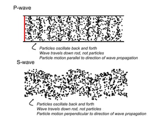
1. P-wave
S-wave
Particles oscillate back and forth
Wave travels down rod, not particles
Particle motion parallel to direction of wave propagation
Particles oscillate back and forth
Wave travels down rod, not particles
Particle motion perpendicular to direction of wave propagation
10. Boundary Effects (Fixed End)
0
0
0
u
Response at boundary is exactly the same as for case
of two waves of same polarity traveling toward each other
At fixed end, displacement is zero and stress is momentarily
doubled. Polarity of reflected wave is same as that of
incident wave
11. Boundary Effects (Fixed End)
0
0
0
u
Response at boundary is exactly the same as for case
of two waves of same polarity traveling toward each other
At fixed end, displacement is zero and stress is momentarily
doubled. Polarity of reflected stress wave is same as that of
incident wave. Polarity of reflected displacement is reversed.
Displacement
21. Boundary Effects (Free End)
0
u
= 0
0
Response at boundary is exactly the same as for case
of two waves of opposite polarity traveling toward each other
At free end, stress is zero and displacement is momentarily
doubled. Polarity of reflected stress wave is opposite that of
incident wave. Polarity of reflected displacement wave is unchanged.
Displacement
22. Boundary Effects (Material Boundaries)
incident
reflected
transmitted
1
1
1
1
1 M
A
E
2
2
2
2
2 M
A
E
29. Boundary Effects (Material Boundaries)
Stiff Soft
Consider limiting condition: v2 0
z = 0
Ar = Ai
At = 2Ai
Displacement amplitude is unchanged
Displacement amplitude at end of rod
is doubled - free surface effect
30. Boundary Effects (Material Boundaries)
Stiff Soft
Consider limiting condition: v2 0
z = 0
r = - i
t = 0
Polarity of stress is reversed,
amplitude unchanged
Stress is zero - free surface effect
32. Three Dimensional Elastic Solids
x
y
z
xx
yy
zz
xy
yx
zy
xz
zy
zx
z
y
x
t
u xz
xy
xx
2
2
z
y
x
t
v yxz
yxy
yx
2
2
z
y
x
t
w zz
zy
zx
2
2
Displacements on left
Stresses on right
33. x
x
t
2
2
2
2
2
2
)
2
(
t
Three Dimensional Elastic Solids
u
x
t
u 2
2
2
)
(
v
y
t
v 2
2
2
)
(
w
z
t
w 2
2
2
)
(
x
s
x
v
t
2
2
2
2
2
2
2
2
p
v
t
)
2
(
p
v
s
v
or
Using 3-dimensional
stress-strain and
strain-displacement
relationships
34. u
x
t
u 2
2
2
)
(
v
y
t
v 2
2
2
)
(
w
z
t
w 2
2
2
)
(
x
x
t
2
2
2
2
2
2
)
2
(
t
Three Dimensional Elastic Solids
x
s
x
v
t
2
2
2
2
2
2
2
2
p
v
t
)
2
(
p
v
s
v
or
Two types of waves can exist in
an infinite body
• p-waves
• s-waves
35. Waves in a Layered Body
Incident P
transmitted P
reflected P
Waves perpendicular to boundaries
p-waves
39. Incident SH
Refracted SH
Reflected SH
Inclined Waves
Incident SH-wave
When wave passes from
stiff to softer material, it is
refracted to a path closer
to being perpendicular to
the layer boundary
Waves in a Layered Body
40. Vs=2,500 fps
Vs=2,000 fps
Vs=1,500 fps
Vs=1,000 fps
Vs=500 fps
Waves in a Layered Body
Waves are nearly
vertical by the time
they reach the
ground surface
41. Waves in a Semi-infinite Body
• The earth is obviously not an infinite body.
• For near-surface earthquake engineering problems
the earth is idealized as a semi-infinite body with
a planar free surface
H1
H2
H3
incident
reflected
Surface wave
Free surface
44. Horizontal and vertical motion of Rayleigh waves
Rayleigh-waves
Rayleigh wave amplitude
decreases quickly with depth
45. Attenuation of Stress Waves
The amplitudes of stress waves in real
materials decrease, or attenuate, with
distance
Material damping
Radiation damping
Two primary sources:
46. Material damping
A portion of the elastic energy of stress
waves is lost due to heat generation
Specific energy decreases as
the waves travel through the material
Consequently, the amplitude of the stress
waves decreases with distance
Attenuation of Stress Waves
47. Radiation damping
The specific energy can also decrease
due to geometric spreading
Consequently, the amplitude of the stress
waves decreases with distance even though
the total energy remains constant
Attenuation of Stress Waves
48. Attenuation of Stress Waves
Both types of damping are important, though one
may dominate the other in specific situations
49. Transfer Function
• A Transfer function may be viewed as a filter that acts upon
some input signal to produce an output signal.
• The transfer function determines how each frequency
in the bedrock (input) motion is amplified, or deamplified
by the soil deposit.
Transfer Function
(filter)
input output
50. Transfer Function
Linear elastic layer on rigid base
u
z
H
u(0,t)
u(H,t)
Aei(wt+kz)
Bei(wt-kz)
At free surface (z = 0),
u(z, t) = 2Acos kz eiwt
t(0, t) = 0 g(0, t) = 0 A = B
Factor of 2 amplification
51. Linear elastic layer on rigid base
u
z
H
u(0,t)
u(H,t)
V
H
H
k
H
z
u
z
u
H
s
*
*
cos
1
cos
1
)
(
)
0
(
)
(
w
w
2
2
cos
1
)
(
s
s V
H
V
H
H
w
w
w
Amplification factor
Transfer function
relates input
to output
Transfer Function
52. Zero damping
Linear elastic layer on rigid base
u
z
H
u(0,t)
u(H,t)
For undamped systems,
infinite amplification can occur
Extremely high amplification occurs
over narrow frequency bands
Amplification is sensitive to
frequency
Fundamental
frequency
Characteristic site period
Ts = 4H
Vs
Transfer Function
53. Linear elastic layer on rigid base
u
z
H
u(0,t)
u(H,t)
Very high, but not infinite,
amplification can occur
Degree of amplification decreases
with increasing frequency
Amplification is still sensitive
to frequency
1% damping
Transfer Function
54. Linear elastic layer on rigid base
u
z
H
u(0,t)
u(H,t)
2% damping
Transfer Function
55. Linear elastic layer on rigid base
u
z
H
u(0,t)
u(H,t)
5% damping
Transfer Function
56. Linear elastic layer on rigid base
u
z
H
u(0,t)
u(H,t)
10% damping
Transfer Function
57. Linear elastic layer on rigid base
u
z
H
u(0,t)
u(H,t)
20% damping
Maximum level of amplification
is low
Amplification sensitive to
fundamental frequency
Transfer Function
58. Linear elastic layer on rigid base
u
z
H
u(0,t)
u(H,t)
All damping
Amplification
De-amplification
Transfer Function
59. Linear elastic layer on rigid base
u
z
H
u(0,t)
u(H,t)
10% damping
Stiffer, thinner
Transfer Function
61. How is it used?
Input motion convolved with transfer function – multiplication in freq domain
Steps:
1. Express input motion as sum of series of sine waves (Fourier series)
2. Multiply each term in series by corresponding term of transfer function
3. Sum resulting terms to obtain output motion.
Notes:
1. Some terms (frequencies) amplified, some de-amplified
2. Amplification/de-amp. behavior depends on position of transfer function
Transfer Function