1. The Thirty-Fourth AAAI Conference on Artificial Intelligence (AAAI-20)
Spatial-Temporal Synchronous Graph Convolutional Networks:
A New Framework for Spatial-Temporal Network Data Forecasting
Chao Song,1,2
Youfang Lin,1,2,3
Shengnan Guo,1,2
Huaiyu Wan1,2,3∗
1
School of Computer and Information Technology, Beijing Jiaotong University, Beijing, China
2
Beijing Key Laboratory of Traffic Data Analysis and Mining, Beijing, China
3
CAAC Key Laboratory of Intelligent Passenger Service of Civil Aviation, Beijing, China
{chaosong, yflin, guoshn, hywan}@bjtu.edu.cn
Abstract
Spatial-temporal network data forecasting is of great impor-
tance in a huge amount of applications for traffic manage-
ment and urban planning. However, the underlying complex
spatial-temporal correlations and heterogeneities make this
problem challenging. Existing methods usually use separate
components to capture spatial and temporal correlations and
ignore the heterogeneities in spatial-temporal data. In this
paper, we propose a novel model, named Spatial-Temporal
Synchronous Graph Convolutional Networks (STSGCN), for
spatial-temporal network data forecasting. The model is able
to effectively capture the complex localized spatial-temporal
correlations through an elaborately designed spatial-temporal
synchronous modeling mechanism. Meanwhile, multiple
modules for different time periods are designed in the model
to effectively capture the heterogeneities in localized spatial-
temporal graphs. Extensive experiments are conducted on
four real-world datasets, which demonstrates that our method
achieves the state-of-the-art performance and consistently
outperforms other baselines.
Introduction
Spatial-temporal network data forecasting is a fundamen-
tal research problem in spatial-temporal data mining. The
spatial-temporal network is a typical data structure that can
describe lots of data in many real-world applications, such as
traffic networks, mobile base-station networks, urban water
systems, etc. Accurate predictions of spatial-temporal net-
work data can significantly improve the service quality of
these applications. With the development of deep learning
on graphs, powerful methods like graph convolutional net-
works and its variants have been widely applied to these
spatial-temporal network data prediction tasks and achieved
promising performance. However, there is still a lack of ef-
fective methods to model the correlations and heterogeneity
in both the spatial and temporal aspects. In this paper, we fo-
cus on designing a model to synchronously capture the com-
plex spatial-temporal correlations and take the heterogeneity
into account to improve the accuracy of spatial-temporal net-
work data forecasting.
∗
Corresponding author: hywan@bjtu.edu.cn
Copyright c
2020, Association for the Advancement of Artificial
Intelligence (www.aaai.org). All rights reserved.
ݐଶ
7LPH
ݐଵ
7HPSRUDOFRUUHODWLRQ
6SDWLDOGHSHQGHQF
6SDWLDOWHPSRUDOFRUUHODWLRQ
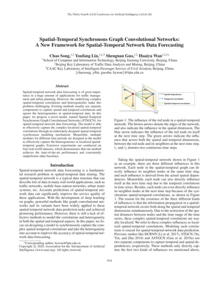
Figure 1: The influence of the red node in a spatial-temporal
network. The brown arrows denote the edges of the network,
and also indicate the influence in the spatial dimension. The
blue arrow indicates the influence of the red node on itself
at the next time step. The green arrows indicate the influ-
ence that across both the spatial and temporal dimensions,
between the red node and its neighbors at the next time step.
t1 and t2 denotes two continuous time steps.
Taking the spatial-temporal network shown in Figure 1
as an example, there are three different influences in this
network. Each node in the spatial-temporal graph can di-
rectly influence its neighbor nodes at the same time step,
and such influence is derived from the actual spatial depen-
dencies. Meanwhile, each node can also directly influence
itself at the next time step due to the temporal correlations
in time series. Besides, each node can even directly influence
its neighbor nodes at the next time step because of the syn-
chronous spatial-temporal correlations, as shown in Figure
1. The reason for the existence of the three different kinds
of influences is that the information propagation in a spatial-
temporal network occurs both along the spatial and temporal
dimensions simultaneously. Due to the restriction of the spa-
tial distances between nodes and the time range of the time
series, these complex spatial-temporal correlations are usu-
ally localized. We refer to these complex influences as local-
ized spatial-temporal correlations. Modeling such correla-
tions is crucial for spatial-temporal network data prediction.
Previous studies like DCRNN (Li et al. 2017), STGCN (Yu,
Yin, and Zhu 2018) and ASTGCN (Guo et al. 2019a) use
two separate components to capture temporal and spatial de-
pendencies, respectively. These methods only directly cap-
ture the first two kinds of influences we mentioned above,
914
2. namely the spatial dependencies and the temporal correla-
tions. They feed the spatial representations into the tempo-
ral modeling modules to capture the third kind of influence
indirectly. However, we believe that if these complex local-
ized spatial-temporal correlations can be captured simulta-
neously, it will be very effective for spatial-temporal data
prediction because this modeling method exposes the fun-
damental way how spatial-temporal network data are gener-
ated.
Besides, spatial-temporal network data usually exhibit
heterogeneity in both the spatial and temporal dimensions.
For example, in a citywide road network, the observations
recorded by traffic monitoring stations in residential and
commercial areas tend to exhibit different patterns at differ-
ent times. However, many previous studies use shared mod-
ules for different time periods, which cannot effectively cap-
ture the heterogeneity in spatial-temporal networks.
To capture the complex localized spatial-temporal cor-
relations and the heterogeneity in spatial-temporal data,
we propose a model called Spatial-Temporal Synchronous
Graph Convolutional Network (STSGCN). Different from
many previous works, the STSGCN model can simulta-
neously capture the localized spatial-temporal correlations
directly, instead of using different types of deep neural
networks to model the spatial dependencies and tempo-
ral correlations separately. Specifically, we construct local-
ized spatial-temporal graphs which connect individual spa-
tial graphs of adjacent time steps into one graph. Then we
construct a Spatial-Temporal Synchronous Graph Convo-
lutional Module (STSGCM) to capture the complex local-
ized spatial-temporal correlations in these localized spatial-
temporal graphs. Meanwhile, to capture the heterogeneity
in long-range spatial-temporal network data, we design a
Spatial-Temporal Synchronous Graph Convolutional Layer
(STSGCL), which deploys multiple individual STSGCMs
on different time periods. Finally, we stack multiple STS-
GCLs to aggregate long-range spatial-temporal correlations
and heterogeneity for prediction.
Overall, the contributions of our work are as follows:
• We propose a novel spatial-temporal graph convolutional
module to synchronously capture the localized spatial-
temporal correlations directly, instead of using different
types of neural network modules separately.
• We construct a multi-module layer to capture the hetero-
geneity in long-range spatial-temporal graphs. This multi-
module layer deploys multiple modules on each time pe-
riod, allowing each module to focus on extracting spatial-
temporal correlations on each localized spatial-temporal
graph.
• Extensive experiments are conducted on four real-world
datasets and the experimental results show that our model
consistently outperforms all the baseline methods.
Related Work
Spatial-Temporal Prediction
The spatial-temporal data prediction problem is a very im-
portant research topic in spatial-temporal data mining. Many
of classic methods like ARIMA (Williams and Hoel 2003)
and SVM (Drucker et al. 1997) only take temporal informa-
tion into account. It is challenging to integrate complex spa-
tial dependencies into prediction methods. The ConvLSTM
(Shi et al. 2015) model is an extension of fully-connected
LSTM (Graves 2013), which combines CNN and RNN to
model spatial and temporal correlations respectively. It uti-
lizes CNN’s powerful capability in spatial information ex-
traction. ST-ResNet (Zhang, Zheng, and Qi 2017) is a CNN
based deep residual network for citywide crowd flows pre-
diction, which shows the power of deep residual CNN on
modeling spatial-temporal grid data. ST-3DNet (Guo et al.
2019b) introduces 3D convolutions into this area, which can
effectively extract features from both the spatial and tem-
poral dimensions. It uses two components to model the lo-
cal temporal patterns and the long-term temporal patterns
respectively. All of these methods above are designed for
spatial-temporal grid data.
Recently, researchers try to utilize graph convolution
methods to model the spatial correlations in spatial-temporal
network data. DCRNN (Li et al. 2017) introduces graph con-
volutional networks into spatial-temporal network data pre-
diction, which employs a diffusion graph convolution net-
work to describe the information diffusion process in spa-
tial networks. It uses RNN to model temporal correlations
like ConvLSTM. STGCN (Yu, Yin, and Zhu 2018) uses
CNN to model temporal correlations. ASTGCN (Guo et al.
2019a) uses two attention layers to capture the dynamics
of spatial dependencies and temporal correlations. Graph
WaveNet (Wu et al. 2019) designs a self-adaptive matrix to
take the variations of the influence between nodes and their
neighbors into account. It uses dilated casual convolutions
to model the temporal correlations to increase the receptive
field exponentially.
However, all of the above methods used two different
components to capture spatial dependencies and temporal
correlations separately. Differ from them, STG2Seq (Bai et
al. 2019) tries to model spatial-temporal correlations simul-
taneously by using a gated residual GCN module with two
attention mechanisms. However, to some extent, concatenat-
ing features of each node in different time steps obscures
spatial-temporal correlations. And it cannot capture the het-
erogeneity in spatial-temporal data.
Graph Convolution Network
Graph convolutional network (GCN) has achieved extraor-
dinary performance on several different types of tasks based
on the graph structure, such as node classification and net-
work representation. Spectral GCNs are defined in the spec-
tral domain. Lots of methods are derived from the work of
(Bruna et al. 2013). ChebNet (Defferrard, Bresson, and Van-
dergheynst 2016) is a powerful GCN that utilizes the Cheby-
shev extension to reduce the complexity of laplacians com-
putation. GCN (Kipf and Welling 2017) simplifies ChebNet
to a more simple form and achieves state-of-the-art perfor-
mance on various tasks. Spatial GCN generalizes the tra-
ditional convolutional network from the Euclidean space
to the vertice domain. GraphSAGE (Hamilton, Ying, and
Leskovec 2017) samples a fixed number of neighbors for
915
3. each node in the graph and aggregates the features of their
neighbors and themselves. GAT (Veličković et al. 2018) is a
powerful GCN variant defined in the vertice domain, which
uses attention layers to adjust the importance of neighbor
nodes dynamically.
Preliminaries
• Definition 1: Spatial network G. We use G = (V, E, A)
to denotes a spatial network, where |V | = N is the set of
vertices, N denotes the number of vertices, and E denotes
the set of edges. A is the adjacency matrix of network G.
The spatial network G represents the relationship between
the nodes in the spatial dimension, and the network struc-
ture does not change with time. In our work, this spatial
network can be either directed or undirected.
• Definition 2: Graph signal matrix X
(t)
G ∈ RN×C
, where
C is the number of attribute features, t denotes the time
step. This graph signal matrix represents the observations
of the spatial network G at the time step t.
The problem of spatial-temporal network data fore-
casting can be described as: learning a mapping func-
tion f which maps the historical spatial-temporal net-
work series (X
(t−T +1)
G , X
(t−T +2)
G , . . . , X
(t)
G ) into the
future observations of this spatial-temporal network
(X
(t+1)
G , X
(t+2)
G , . . . , X
(t+T
)
G ), where T denotes the length
of historical spatial-temporal network series, T
denotes the
length of the target spatial-temporal network series to fore-
cast.
Spatial-Temporal Synchronous Graph
Convolutional Network
Figure 2 illustrates the architecture of our STSGCN model.
We summarize the core idea of STSGCN as three points: 1)
Connect each node with itself at the previous and the next
time steps to construct a localized spatial-temporal graph. 2)
Use a Spatial-Temporal Synchronous Graph Convolutional
Module to capture the localized spatial-temporal correla-
tions. 3) Deploy multiple modules to model heterogeneities
in spatial-temporal network series.
Localized Spatial-Temporal Graph Construction
We intend to build a model that can directly capture the im-
pact of each node on its neighbors that belongs to both the
current and the adjacent time steps. The most intuitive idea
to achieve this goal is to connect all nodes with themselves
at the adjacent time steps (Figure 3 (a)). By connecting all
nodes with themselves at the previous and the next moments,
we can get a localized spatial-temporal graph. According
to the topological structure of the localized spatial-temporal
graph, the correlations between each node and its spatial-
temporal neighbors can be captured directly.
We use A ∈ RN×N
to denote the adjacency matrix of the
spatial graph. A
∈ R3N×3N
denotes the adjacency matrix
of the localized spatial-temporal graph constructed on three
continuous spatial graphs. For node i in the spatial graph, we
can calculate its new index in the localized spatial-temporal
676*0
676*/VZLWK
VSDWLDODQGWHPSRUDO
HPEHGGLQJ
,QSXWVSDWLDO
WHPSRUDOQHWZRUN
VHULHV
7DUJHW VSDWLDO
WHPSRUDOQHWZRUN
VHULHV
2XWSXWWUDQVIRUPODHUV
)XOOFRQQHFWHG/DHU ,QSXWWUDQVIRUPODHU
)XOOFRQQHFWHG/DHUV
)XOOFRQQHFWHG/DHUV
676*0
676*0
676*0
676*0
676*0
Figure 2: STSGCN architecture. Our STSGCN consists
of multiple Spatial-Temporal Synchronous Graph Convolu-
tional Layers (STSGCLs) with an input and an output layer.
It uses an input layer to transform the input features into
a higher dimensional space. Then stacked mulitple STSG-
CLs capture the localized spatial-temporal correlations and
heterogeneities in spatial-temporal network series. Finally, it
uses a multi-module output layer to map the final represen-
tations into the output space.
graph by (t − 1)N + i, where t (0 t ≤ 3) denotes the
time step number in the localized spatial-temporal graph. If
two nodes connect with each other in this localized spatial-
temporal graph, the corresponding value in the adjacency
matrix is set to be 1. The adjacency matrix of the localized
spatial-temporal graph can be formulated as:
A
i,j =
1, if vi connects to vj
0, otherwise
, (1)
where vi denotes the node i in localized spatial-temporal
graph. The adjacency matrix A
contains 3N nodes. Figure
3 (b) illustrates the adjacency matrix of the localized spatial-
temporal graph. The diagonal of the adjacency matrix are the
adjacency matrices of the spatial networks of three contin-
uous time steps. The two sides of the diagonal indicate the
connectivity of each node to itself that belongs to the adja-
cent time steps.
Spatial-Temporal Embedding
However, connecting the nodes at different time step into
one graph obscures the time attribute of each node. In other
words, this localized spatial-temporal graph puts the nodes
at different time steps into a same environment without dis-
tinguishing them. Inspired by the ConvS2S(Gehring et al.
2017), we equip position embedding to the spatial-temporal
network series so that the model can take the spatial and
temporal information into account, which can enhance the
ability to model the spatial-temporal correlations. For the
spatial-temporal network series XG ∈ RN×C×T
, we cre-
ate a learnable temporal embedding matrix Temb ∈ RC×T
916
6. $GMDFHQFPDWUL[RI/RFDOL]HG
6SDWLDO7HPSRUDO*UDSK
Figure 3: Localized Spatial-Temporal Graph construction.
(a) is an example of a localized spatial-temporal graph. (b) is
the adjacency matrix of the localized spatial-temporal graph
in (a). A(ti)
denotes the adjacency matrix of the spatial graph
at time step i. Ati→tj
denotes the connections between the
nodes with themselves at the time step i and j.
and a learnable spatial embedding matrix Semb ∈ RN×C
.
After the training process is completed, the two embedding
matrices will contains the necessary temporal and spatial
information to help the model capture the spatial-temporal
correlations.
We add these two embedding matrix to the spatial-
temporal network series with broadcast operation to obtain
the new representations of the network series:
XG+temb+semb
= XG + Temb + Semb ∈ RN×C×T
. (2)
Spatial-Temporal Synchronous Graph
Convolutional Module
We build a Spatial-Temporal Synchronous Graph Convo-
lutional Module (STSGCM) to capture localized spatial-
temporal correlations. The STSGCM consists of a group of
graph convolutional operations. Graph convolutional opera-
tions can aggregate the features of each node with its neigh-
bors. We define a graph convolutional operation in the ver-
tice domain to aggregate localized spatial-temporal features
in spatial-temporal networks. The input of the graph con-
volutional operation is the graph signal matrix of the local-
ized spatial-temporal graph. In our graph convolutional op-
eration, each node aggregates the features of its own and its
neighbors at adjacent time steps. The aggregate function is a
linear combination whose weights are equal to the weights
of the edges between the node and its neighbors. Then we
deploy a fully-connected layer with an activation function to
transform the features of nodes into a new space. This graph
convolutional operation can be formulated as follow:
GCN(h(l−1)
) = h(l)
= σ(A
h(l−1)
W + b) ∈ R3N×C
,
(3)
where A
∈ R3N×3N
denotes the adjacency matrix of the
localized spatial-temporal graph, h(l−1)
∈ R3N×C
is the in-
put of the l-th graph convolutional layer, W ∈ RC×C
and
b ∈ RC
are learnable parameters, σ denotes the activation
function, such as ReLU and GLU (Dauphin et al. 2017). If
we select GLU as the activation function of the graph convo-
lutional layer, the graph convolutional layer can be described
as follow:
h(l)
= (A
h(l−1)
W1 + b1) ⊗ sigmoid(A
h(l−1)
W2 + b2),
(4)
where W1 ∈ RC×C
, W2 ∈ RC×C
, b1 ∈ RC
, b2 ∈ RC
are learnable parameters, sigmoid denotes the sigmoid ac-
tivation function, i.e., sigmoid(x) = 1
1+e−x , ⊗ denotes
element-wise product. The gated linear unit controls which
node’s information can be passed to the next layer.
This graph convolutional operation is defined in the ver-
tice domain, which means that it does not need to compute
the graph laplacian. Also, this graph convolutional operation
can be applied not only to undirected graphs but also to di-
rected graphs. In addition, we add self-loop to each node in
the localized spatial-temporal graph, in order to allow the
graph convolutional operation to take its own characteristics
into account when aggregating features.
We stack multiple graph convolutional operations to ex-
pand the aggregation area, which can increase the receptive
field of the graph convolution operations to capture localized
spatial-temporal correlations (Figure 4 (a)). We select JK-net
(Xu et al. 2018) as the base structure of our STSGCM and
design a new aggregation layer to filter useless information
(Figure 4 (b), 4 (c)).
D
9. URSSLQJRSHUDWLRQ
ݐଷ
ݐଶ
ݐଵ
Figure 4: (a) is an example of the architecture of the Spatial-
Temporal Synchronous Graph Convolutional Module with
two graph convolutional operations. Cin and Cout denotes
the number of features of the input matrix and the output
matrix respectively, AGG denotes the aggregation layer. (b)
denotes the output of the aggregating operation. (c) is an ex-
ample of cropping operation in the aggregation layer, which
only retain the nodes at the middle time step.
We use h(l)
to denote the output of the l-th graph convo-
lutional operation, where h(0)
denotes the input of the first
graph convolutional operation. For STSGCM with L graph
convolutional operations, the output of each graph convolu-
tion operation will be fed into an aggregation layer (Figure
4 (a)). The aggregation layer will compact the outputs of all
917
10. layers in the STSGCM. The aggregation operation has two
steps: aggregating and cropping.
Aggregating operation We select max-pooling as the ag-
gregation operation. It applies an element-wise max opera-
tion to the outputs of all the graph convolutions in STSGCM.
The max operation needs all outputs have the same size, so
the number of the kernels for the graph convolutional opera-
tions within a module should be equal. The max aggregating
operation can be formulated as:
hAGG = max(h(1)
, h(2)
, . . . , h(L)
) ∈ R3N×Cout
, (5)
where Cout denotes the number of kernels in the graph con-
volutional operations.
Cropping operation The cropping operation (Figure 4
(c)) removes all the features of the nodes at the previous
and the next time steps, and only the nodes in the middle
moment are retained. The reason for that is the graph convo-
lutional operations has already aggregated the information
from the previous and the next time steps. Each node con-
tains the localized spatial-temporal correlations even though
we crop the two time steps. If we stack multiple STSGCMs
and retain the features of all the adjacent time steps, much
redundant information will reside in the model, which can
seriously impair the performance of the model.
To sum up, the input to STSGCM is a localized spatial-
temporal graph signal matrix h(0)
∈ R3N×Cin
. After several
graph convolutional operations, the outputs of each graph
convolutional operation can be denoted as h(i)
∈ R3N×Cout
,
where i denotes the operation index. The aggregating oper-
ation will compact them into hAGG ∈ R3N×Cout
. Then the
cropping operation retain the nodes at the middle time step,
generate the output of STSGCM h(final)
∈ RN×Cout
. The
green arrows in Figure 1 indicate the spaital-temporal corre-
lations between the node and its two-hop neighbors in local-
ized spatial-temporal graphs. The STSGCMs with at least
two stacked graph convolutional operations can model the
three different types of correlations indicated in Figure 1 di-
rectly.
Spatial-Temporal Synchronous Graph
Convolutional Layer
To capture long-range spatial-temporal correlations of the
entire network series, we use a sliding window to cut out
different periods. Due to the heterogeneity in the spatial-
temporal data, it is better to use multiple STSGCMs to
model different periods rather than to share one for all pe-
riods. Multiple STSGCMs allow each one to focus on mod-
eling the localized spatial-temporal correlations in the local-
ized graph. We deploy a group of STSGCMs as a Spatial-
Temporal Synchronous Graph Convolutional Layer (STS-
GCL) to extract long-range spatial-temporal features, as
shown in Figure 2.
We denote the input matrix of a STSGCL as X ∈
RT ×N×C
. We add spatial-temporal embeddings for each
STSGCL at first. Then the sliding window in the STSGCL
will cuts out the input into T − 2 spatial-temporal network
series. Each spatial-temporal network series can be denoted
as X
∈ R3×N×C
. We reshape them as X
reshape ∈ R3N×C
,
which can be fed into STSGCM with the localized spatial-
temporal graph directly. STSGCL deploys T −2 STSGCMs
on T −2 localized spatial-temporal graphs to capture the lo-
calized spatial-temporal correlations in these T − 2 spatial-
temporal network series. After that, all these T − 2 STS-
GCMs’ outputs are concatenated into one matrix as the out-
put of STSGCL. That can be formulated as:
M = [M1, M2, . . . , MT −2] ∈ R(T −2)×N×Cout
, (6)
where Mi ∈ RN×Cout
denotes the outputs of the i-th STS-
GCM.
By stacking multiple STSGCLs, we can build a hierar-
chical model that can capture complex spatial-temporal cor-
relations and spatial-temporal heterogeneity. After several
spatial-temporal synchronous graph convolution operations,
each node will contain the localized spatial-temporal corre-
lations centered by itself.
Extra Components
In this section, we introduce some extra components that the
STSGCN equiped to enhance its representation power.
Mask matrix For the graph convolutional operations in
STSGCN, the adjacency matrix A
decides the weights of
aggregation. However, each node has a different influence
magnitude on its neighbors. If the adjacency matrix only
contains 0 and 1, the aggregation may be restricted. If the
two nodes in the localized spatial-temporal graph are con-
nected, even if they have no correlation at a certain period,
their features will be aggregated. So we add a learnable mask
matrix Wmask in STSGCN to adjust the aggregation weights
to make the aggregation more reasonable.
Wmask ∈ R3N×3N
denotes the mask matrix. We do the
element-wise product between Wmask and localized adja-
cency matrix A
to generate a weight adjusted localized ad-
jacency matrix:
A
adjusted = Wmask ⊗ A
∈ R3N×3N
. (7)
After that, we use A
adjusted to compute all graph convo-
lutions in our model.
Input layer We add a fully connected layer at the top of
the network to transform the input into a high-dimension
space, which can improve the representation power of the
network.
Output layer We design an output layer to transform the
output of the last STSGCL into the expected prediction. The
input of this output layer can be denoted as X ∈ RT ×N×C
.
We first transpose and reshape it to X
∈ RN×T C
. Then we
use T
two-fully-connected-layers to generate the prediction
as follow:
ŷ(i)
= ReLU(X
W
(i)
1 + b
(i)
1 ) · W
(i)
2 + b
(i)
2 , (8)
where ŷ(i)
denotes the prediction in time step i. W
(i)
1 ∈
RT C×C
, b
(i)
1 ∈ RC
, W
(i)
2 ∈ RC
×1
, b
(i)
2 ∈ R are learnable
918
11. Table 1: Dataset description.
Datasets Number of sensors Time range
PEMS03 358 9/1/2018 - 11/30/2018
PEMS04 307 1/1/2018 - 2/28/2018
PEMS07 883 5/1/2017 - 8/31/2017
PEMS08 170 7/1/2016 - 8/31/2016
parameters, C
denotes the number of features of the output
of the first fully-connected layer. Then we concatenate all
predictions of each time step into one matrix:
Ŷ = [ŷ(1)
, ŷ(2)
, . . . , ŷ(T )
] ∈ RN×T
, (9)
where Ŷ is the output of the overall STSGCN.
Loss function We select Huber loss (Huber 1992) as the
loss function. The Huber loss is less sensitive to outliers than
the squared error loss.
L(Y, Ŷ ) =
1
2 (Y − Ŷ )2
|Y − Ŷ | ≤ δ
δ|Y − Ŷ | − 1
2 δ2
otherwise
, (10)
where Y denotes the ground truth and Ŷ denotes the predic-
tion of the model, δ is a threshold parameter which controls
the range of squared error loss.
Experiments
We evaluate the performance of STSGCN on four high-
way traffic datasets. These data are collected from the Cal-
trans Performance Measurement System (PeMS) (Chen et
al. 2001).
Datasets
We construct four different datasets from 4 districts respec-
tively, namely PEMS03, PEMS04, PEMS07 and PEMS08.
The flow data is aggregated to 5 minutes, which means there
are 12 points in the flow data for each hour. We use traffic
flow data from the past hour to predict the flow for the next
hour. The detailed information is shown in Table 1.
The spatial networks for each dataset is constructed ac-
cording to the actual road network. If the two monitors are
on the same road, the two points are considered to be con-
nected in the spatial network.
We standardize the features by removing the mean and
scaling to unit variance with:
X
=
X − mean(X)
std(X)
(11)
where mean(X) and std(X) are the mean and the standard
deviation of the historical time series, respectively.
Baseline Methods
• VAR (Hamilton 1994): Vector Auto-Regression is an ad-
vanced time series model, which can capture the pairwise
relationships among time series.
• SVR (Drucker et al. 1997): Support Vector Regression
uses a linear support vector machine for regression tasks.
• LSTM (Hochreiter and Schmidhuber 1997): Long Short-
Term Memory Network for time series prediction.
• DCRNN (Li et al. 2017): Diffusion Convolutional Re-
current Neural Network utilizes diffusion graph convolu-
tional networks and seq2seq to encode spatial information
and temporal information, respectively.
• STGCN (Yu, Yin, and Zhu 2018): Spatial-Temporal
Graph Convolutional Network. STGCN uses ChebNet
and 2D convolutional networks to capture spatial depen-
dencies and temporal correlations, respectively.
• ASTGCN(r) (Guo et al. 2019a): Attention Based Spatial-
Temporal Graph Convolutional Networks designs spatial
attention and temporal attention mechanisms to model
spatial and temporal dynamics, respectively. ASTGCN in-
tegrates three different components to model periodicity
of highway traffic data. In order to ensure the fairness of
comparison experiments, we only take its recent compo-
nents.
• STG2Seq (Bai et al. 2019): Spatial-Temporal Graph to
Sequence Model uses multiple gated graph convolutional
module and seq2seq architecture with attention mecha-
nisms to make multi-step prediction.
• Graph WaveNet (Wu et al. 2019): Graph WaveNet com-
bines graph convolution with dilated casual convolution
to capture spatial-temporal dependencies.
Experiment Settings
We split all datasets with ratio 6 : 2 : 2 into training sets,
validation sets and test sets. We use one hour historical data
to predict the next hour’s data, which means using the past
12 continuous time steps to predict the future 12 continuous
time steps. All experiments are repeated ten times.
We implement the STSGCN model using MXNet (Chen
et al. 2015). The hyperparameters are determined by the
model’s performance on the validation datasets. The best
model on these four datasets consists of 4 STSGCLs, each
STSGCM contains 3 graph convolutional operations with
64, 64, 64 filters respectively.
Experiment Results
Table 2 shows the comparsion of different approaches for
the forecasting tasks. Our STSGCN consistently outper-
forms other baseline methods on three datasets except for
PEMS07. In PEMS07, our STSGCN has the best MAE and
MAPE, except for the RMSE which is slightly larger than
the that of DCRNN.
VAR, SVM and LSTM only take temporal correlations
into consideration and cannot utilize the spatial dependen-
cies of the spatial-temporal network. DCRNN, STGCN,
ASTGCN(r), STG2Seq and our STSGCN all take advan-
tages of spatial information, so they have better performance
than the methods only for time series prediction.
DCRNN, STGCN, ASTGCN, and Graph WaveNet use
two module to model spatial dependencies and temporal cor-
relations respectively. And they share one module with all
919
12. Table 2: Performance comparison of different approaches for traffic flow forecasting.
Baseline methods
VAR SVR LSTM DCRNN STGCN ASTGCN(r) STG2Seq Graph WaveNet STSGCN
Datasets Metrics
PEMS03
MAE 23.65 21.97 ± 0.00 21.33 ± 0.24 18.18 ± 0.15 17.49 ± 0.46 17.69 ± 1.43 19.03 ± 0.51 19.85 ± 0.03 17.48 ± 0.15
MAPE (%) 24.51 21.51 ± 0.46 23.33 ± 4.23 18.91 ± 0.82 17.15 ± 0.45 19.40 ± 2.24 21.55 ± 1.68 19.31 ± 0.49 16.78 ± 0.20
RMSE 38.26 35.29 ± 0.02 35.11 ± 0.50 30.31 ± 0.25 30.12 ± 0.70 29.66 ± 1.68 29.73 ± 0.52 32.94 ± 0.18 29.21 ± 0.56
PEMS04
MAE 23.75 28.70 ± 0.01 27.14 ± 0.20 24.70 ± 0.22 22.70 ± 0.64 22.93 ± 1.29 25.20 ± 0.45 25.45 ± 0.03 21.19 ± 0.10
MAPE (%) 18.09 19.20 ± 0.01 18.20 ± 0.40 17.12 ± 0.37 14.59 ± 0.21 16.56 ± 1.36 18.77 ± 0.85 17.29 ± 0.24 13.90 ± 0.05
RMSE 36.66 44.56 ± 0.01 41.59 ± 0.21 38.12 ± 0.26 35.55 ± 0.75 35.22 ± 1.90 38.48 ± 0.50 39.70 ± 0.04 33.65 ± 0.20
PEMS07
MAE 75.63 32.49 ± 0.00 29.98 ± 0.42 25.30 ± 0.52 25.38 ± 0.49 28.05 ± 2.34 32.77 ± 3.21 26.85 ± 0.05 24.26 ± 0.14
MAPE (%) 32.22 14.26 ± 0.03 13.20 ± 0.53 11.66 ± 0.33 11.08 ± 0.18 13.92 ± 1.65 20.16 ± 4.36 12.12 ± 0.41 10.21 ± 0.05
RMSE 115.24 50.22 ± 0.01 45.84 ± 0.57 38.58 ± 0.70 38.78 ± 0.58 42.57 ± 3.31 47.16 ± 3.66 42.78 ± 0.07 39.03 ± 0.27
PEMS08
MAE 23.46 23.25 ± 0.01 22.20 ± 0.18 17.86 ± 0.03 18.02 ± 0.14 18.61 ± 0.40 20.17 ± 0.49 19.13 ± 0.08 17.13 ± 0.09
MAPE (%) 15.42 14.64 ± 0.11 14.20 ± 0.59 11.45 ± 0.03 11.40 ± 0.10 13.08 ± 1.00 17.32 ± 1.14 12.68 ± 0.57 10.96 ± 0.07
RMSE 36.33 36.16 ± 0.02 34.06 ± 0.32 27.83 ± 0.05 27.83 ± 0.20 28.16 ± 0.48 30.71 ± 0.61 31.05 ± 0.07 26.80 ± 0.18
different periods to extract the long-range spatial-temporal
correlations, which ignores the heterogeneities in spatial-
temporal network data. Our method take localized spatial-
temporal correlations into account and capture the hetero-
geneities in spatial-temporal data, so our STSGCN has bet-
ter performance than these methods.
STG2Seq also intends to model the spatial-temporal cor-
relations simultaneously. As we can see from the Table 2,
our STSGCN has better performance on the four datasets.
The limitation of STG2Seq is that it simply concatenates the
features of the neighboring periods, rather than treating the
nodes at different time steps as different individual nodes
like our STSGCN. To some extent this approach ignores
temporal information and spatial-temporal correlations.
Component Analysis
To further investigate the effect of different modules of STS-
GCN, we design six variants of the STSGCN model. We
compare these six variants with the STSGCN model on the
PEMS03 dataset. All of these models contains four STSG-
CLs with [64, 64, 64] filters in each STSGCM. The differ-
ence of these seven models are described as below:
1. basic: This model does not equip with spatial-temporal
embeddings and mask matrix. It uses ReLU as the acti-
vation function. Each STSGCL only contains one STS-
GCM, and it shares this module in all time periods. The
output layer is the same as ASTGCN’s output layer which
simply uses a convolutional layer with 12 filters to gener-
ate predictions.
2. mulit-module: This model changes the STSGCLs in the
basic model to multi-module version.
Figure 5: Component analysis of STSGCN.
3. GLU: This model changes all of activation function in
multi-module model to GLU.
4. +emb: This model adds spatial-temporal embeddings in
each STSGCL based on GLU version.
5. +mask: This model adds mask matrix based on +emb.
6. reshape-output: This model uses two fully connected lay-
ers to generate the expected predictions.
7. STSGCN: The STSGCN model deploys multiple two-
fully-connected layers to generate predictions of each
time step.
As Figure 5 illustrates, the GLU have better performance
than ReLU activation function. The reason for that is GLU
has twice the parameter size of ReLU, so its larger capacity
enables it to captures complex spatial-temporal correlations.
Besides, it can control the output more flexibly than ReLU.
The model that equips with individual STSGCMs for each
time period outperforms the shared STSGCM by a large
margin, which shows the necessity of modeling the hetero-
geneities in spatial-temporal network data.
Besides, the results show that the spatial-temporal embed-
ding can obviously improve the performance of the STS-
GCN model.
We add the mask matrix to tune the weights between each
node and its neighbors in graph convolution operations. It
can improve the forecasting performance a little.
The convolutional layer for generating the prediction does
not make sense, because it shares all the parameters with all
nodes in spatial graphs. Due to the heterogeneity in spatial-
temporal data, each node may exhibit different properties, so
using different modules to generate the prediction results is
better than one convolutional output layer. So the reshaped
output layer and multi-output version can further improve
the prediction performance.
Conclusion
We propose a model which can not only capture the lo-
calized spatial-temporal correlations effectively but also
take the heterogeneities in spatial-temporal data into con-
siderations. And extensive experiments on four real-world
datasets show that our model is superior to the exist-
ing models. Besides, our proposed model is a general-
framework for spatial-temporal network data forecast-
920
13. ing, so it can be applied in many related applica-
tions. The code and datasets have been released at:
https://github.com/Davidham3/STSGCN.
Acknowledgments
This work was supported by the Fundamental Re-
search Funds for the Central Universities (Grant No.
2019JBM024).
References
Bai, L.; Yao, L.; Kanhere, S.; Wang, X.; and Sheng, Q.
2019. Stg2seq: Spatial-temporal graph to sequence model
for multi-step passenger demand forecasting. In IJCAI.
Bruna, J.; Zaremba, W.; Szlam, A.; and LeCun, Y. 2013.
Spectral networks and locally connected networks on
graphs. CoRR abs/1312.6203.
Chen, C.; Petty, K.; Skabardonis, A.; Varaiya, P.; and Jia,
Z. 2001. Freeway performance measurement system: min-
ing loop detector data. Transportation Research Record
1748(1):96–102.
Chen, T.; Li, M.; Li, Y.; Lin, M.; Wang, N.; Wang, M.; Xiao,
T.; Xu, B.; Zhang, C.; and Zhang, Z. 2015. Mxnet: A flexi-
ble and efficient machine learning library for heterogeneous
distributed systems. ArXiv abs/1512.01274.
Dauphin, Y. N.; Fan, A.; Auli, M.; and Grangier, D. 2017.
Language modeling with gated convolutional networks. In
Proceedings of the 34th International Conference on Ma-
chine Learning-Volume 70, 933–941. JMLR. org.
Defferrard, M.; Bresson, X.; and Vandergheynst, P. 2016.
Convolutional neural networks on graphs with fast localized
spectral filtering. In Advances in neural information pro-
cessing systems, 3844–3852.
Drucker, H.; Burges, C. J.; Kaufman, L.; Smola, A. J.; and
Vapnik, V. 1997. Support vector regression machines. In Ad-
vances in neural information processing systems, 155–161.
Gehring, J.; Auli, M.; Grangier, D.; Yarats, D.; and Dauphin,
Y. N. 2017. Convolutional sequence to sequence learning.
In Proceedings of the 34th International Conference on Ma-
chine Learning-Volume 70, 1243–1252. JMLR. org.
Graves, A. 2013. Generating sequences with recurrent neu-
ral networks. arXiv preprint arXiv:1308.0850.
Guo, S.; Lin, Y.; Feng, N.; Song, C.; and Wan, H. 2019a. At-
tention based spatial-temporal graph convolutional networks
for traffic flow forecasting. In Proceedings of the AAAI Con-
ference on Artificial Intelligence, volume 33, 922–929.
Guo, S.; Lin, Y.; Li, S.; Chen, Z.; and Wan, H. 2019b. Deep
spatial-temporal 3d convolutional neural networks for traffic
data forecasting. IEEE Transactions on Intelligent Trans-
portation Systems.
Hamilton, W.; Ying, Z.; and Leskovec, J. 2017. Inductive
representation learning on large graphs. In Advances in Neu-
ral Information Processing Systems, 1024–1034.
Hamilton, J. D. 1994. Time series analysis, volume 2.
Princeton university press Princeton, NJ.
Hochreiter, S., and Schmidhuber, J. 1997. Long short-term
memory. Neural computation 9(8):1735–1780.
Huber, P. J. 1992. Robust estimation of a location parameter.
In Breakthroughs in statistics. Springer. 492–518.
Kipf, T. N., and Welling, M. 2017. Semi-supervised classi-
fication with graph convolutional networks. In International
Conference on Learning Representations (ICLR).
Li, Y.; Yu, R.; Shahabi, C.; and Liu, Y. 2017. Diffusion
convolutional recurrent neural network: Data-driven traffic
forecasting. In ICLR.
Shi, X.; Chen, Z.; Wang, H.; Yeung, D.-Y.; Wong, W.-K.;
and Woo, W.-c. 2015. Convolutional lstm network: A ma-
chine learning approach for precipitation nowcasting. In Ad-
vances in neural information processing systems, 802–810.
Veličković, P.; Cucurull, G.; Casanova, A.; Romero, A.; Liò,
P.; and Bengio, Y. 2018. Graph Attention Networks. Inter-
national Conference on Learning Representations. accepted
as poster.
Williams, B. M., and Hoel, L. A. 2003. Modeling and fore-
casting vehicular traffic flow as a seasonal arima process:
Theoretical basis and empirical results. Journal of trans-
portation engineering 129(6):664–672.
Wu, Z.; Pan, S.; Long, G.; Jiang, J.; and Zhang, C. 2019.
Graph wavenet for deep spatial-temporal graph modeling.
In IJCAI.
Xu, K.; Li, C.; Tian, Y.; Sonobe, T.; ichi Kawarabayashi, K.;
and Jegelka, S. 2018. Representation learning on graphs
with jumping knowledge networks. In ICML.
Yu, B.; Yin, H.; and Zhu, Z. 2018. Spatio-temporal graph
convolutional networks: A deep learning framework for traf-
fic forecasting. In IJCAI.
Zhang, J.; Zheng, Y.; and Qi, D. 2017. Deep spatio-temporal
residual networks for citywide crowd flows prediction. In
Thirty-First AAAI Conference on Artificial Intelligence.
921