Electromagnetic relays used for power system .pptx
energies-11-00540-v2 (1).pdf
1. energies
Article
Modified Differential Evolution Algorithm: A Novel
Approach to Optimize the Operation of
Hydrothermal Power Systems while Considering the
Different Constraints and Valve Point Loading Effects
Thang Trung Nguyen 1 ID
, Nguyen Vu Quynh 2 ID
, Minh Quan Duong 3 ID
and Le Van Dai 4,5,* ID
1 Power System Optimization Research Group, Faculty of Electrical and Electronics Engineering,
Ton Duc Thang University, Ho Chi Minh City 700000, Vietnam; nguyentrungthang@tdt.edu.vn
2 Department of Electrical Engineering, Lac Hong University, Bien Hoa 810000, Vietnam;
vuquynh@lhu.edu.vn
3 Department of Electrical Engineering, The University of Da Nang—University of Science and Technology,
Danang 550000, Vietnam; dmquan@dut.udn.vn
4 Institute of Research and Development, Duy Tan University, Danang 550000, Vietnam
5 Office of Science Research and Development, Lac Hong University, Bien Hoa 810000, Vietnam
* Correspondence: levandai@duytan.edu.vn; Tel.: +84-901-672-689
Received: 1 January 2018; Accepted: 24 February 2018; Published: 2 March 2018
Abstract: This paper proposes an efficient and new modified differential evolution algorithm
(ENMDE) for solving two short-term hydrothermal scheduling (STHTS) problems. The first is
to take the available water constraint into account, and the second is to consider the reservoir
volume constraints. The proposed method in this paper is a new, improved version of the
conventional differential evolution (CDE) method to enhance solution quality and shorten the
maximum number of iterations based on two new modifications. The first focuses on a self-tuned
mutation operation to open the local search zone based on the evaluation of the quality of the solution,
while the second focuses on a leading group selection technique to keep a set of dominant solutions.
The contribution of each modification to the superiority of the proposed method over CDE is also
investigated by implementing CDE with the self-tuned mutation (STMDE), CDE with the leading
group selection technique (LGSDE), and CDE with the two modifications. In addition, particle swarm
optimization (PSO), the bat algorithm (BA), and the flower pollination algorithm (FPA) methods are
also implemented through four study cases for the first problem, and two study cases for the second
problem. Through extensive numerical study cases, the effectiveness of the proposed approach
is confirmed.
Keywords: self-tuned mutation; leading group selection; available water constraints; non-convex
objective; reservoir volume constraints
1. Introduction
An electrical power system is mainly composed of thermal and hydro power plants connected
via transmission lines in order to supply electricity to loads such as industrial zones or manufacturers,
etc. For electrical generation, thermal plants use fossil fuel including gas, coal, and oil, which are very
expensive, and will become exhausted in the near future, whereas taking water from natural rivers
and discharging it via hydro turbines is considered negligible in terms of generation costs. In addition,
comparing the response speed to electrical load changes, hydropower plants have advantages over
thermal plants, because they can move from producing a very small amount of power to full power in
several minutes, due to the quick water control. On the contrary, the startup and the response speed of
Energies 2018, 11, 540; doi:10.3390/en11030540 www.mdpi.com/journal/energies
2. Energies 2018, 11, 540 2 of 30
thermal plants to load changes is very slow. Therefore, thermal plants need to run continuously for
some hours once they start. Based on the advantages and disadvantages analyzed for thermal and
hydropower plants, it is clear that the coordination of thermal and hydropower plants in electrical
generation operations becomes more effective and economical. In summary, hydrothermal scheduling
(HTS) aims to minimize the electricity generation fuel cost of thermal plants using fossil fuels, while
all constraints from thermal plants, hydropower plants and the system are exactly met [1]. With regard
to this problem, the thermal power plant constraints are easily met, because only limitations on
generation are taken into consideration and other constraints such as fossil fuel constraints and fuel
costs for the start-up and shutdown processes are neglected. Among the optimization problems
related to the optimal scheduling of hydrothermal systems, the fixed-head, short-term HTS problem
has been widely and successfully studied so far [1–29]. The fixed-head, short-term HTS problem
has been classified into two sub-problems with different hydraulic constraints, namely the amount
of discharged water available via the turbine [1–17] and reservoir volume limits [2,3,18–34]. In the
two sub-problems, the water head of reservoirs is not supposed to be changed over the scheduled
time, thus the water discharge function of the two problems has the same quadratic function model
with respect to hydro generation and coefficients; however, the set of hydraulic constraints taken into
account in the problems are almost completely different. The water volume, which is allowed to run
the hydro turbines over the scheduled horizon, is constrained in the first problem, while the main
constraints considered in the second problem are the reservoir volume at the beginning and the end of
the scheduled horizon, the limitations of the reservoir volume and the water balance in each reservoir.
Several methods have been used to solve the first problem, such as Powell’s hybrid method [1]; the
Newton–Raphson method [1,2]; the lambda–gamma method (λ-γ method) [2]; the Lagrange-multiplier,
factorization-based, Newton–Raphson method [3]; the Lagrange method based on the linearization
of the coordination equation (LCEL) [4]; the Lagrangian relaxation approach [5]; Hopfield neural
networks (HNN) [6]; evolutionary programming (EP) [7,8]; the artificial immune system method
(AIS) [8]; particle swarm optimization (PSO) and the differential evolutionary method (DE) [8];
the modified bacterial foraging algorithm (MBFA) [9]; the optimal gamma-based genetic algorithm
(OGB-GA) [10]; fast genetic algorithm (FGA) [11]; the predator–prey optimization technique (PPO) [12];
improved genetic with multiplier updating (IGA-MU) [13]; real-coded genetic algorithm (RCGA) [14];
a Hopfield Lagrange network (HLN) [15]; an augmented Hopfield Lagrange network (ALHN) [15];
the Cuckoo search algorithm (CSA) [16,17]; and a modified cuckoo search algorithm (MCSA) [17].
On the other hand, there has also been a number of methods proposed to solve the second problem,
such as gradient search (GS) [2]; Newton’s method [3]; the simulated annealing approach (SA) [18];
evolutionary programming (EP) [19–21]; genetic algorithms (GA) [22]; fast EP (FEP) [23]; improved fast
EP (IFEP) [23]; hybrid EP (HEP) [24]; PSO [25]; the improved bacterial foraging algorithm (IBFA) [26];
self-organizing, hierarchical PSO [27]; running improved fast EP (RIFEP) [28]; improved PSO [29,30];
a clonal selection algorithm (CS) [31]; fully-informed particle swarm optimization (FIPSO) [32]; a
cuckoo search algorithm with Lévy distribution (CSA-Lévy) [33]; a cuckoo search algorithm with
Lévy Gaussian distribution (CSA-Gauss) [33]; a cuckoo search algorithm with Cauchy distribution
(CSA-Cauchy) [33]; a one rank cuckoo search algorithm with Lévy distribution (ORCSA-Lévy) [34];
and a one rank cuckoo search algorithm with Cauchy distribution (ORCSA-Cauchy) [34].
Among the introduced methods, the methods in [1–6,15] are in the family of deterministic
algorithms and the others in [7–14,16–34] are in the family of meta-heuristic algorithms. The first
method group is mainly based on the gradient to find the optimal solution. Meanwhile the second
method group searches for the optimal solution mainly based on the population. Moreover, the
methods in the first group are defined as derivative-based optimization methods, finding the
optimal solution by a single path search line and suffering from the drawback that they cannot
deal with non-convex problems where the objective functions or constraints of the problems are
non-differentiable or nonlinear. In addition, the conventional methods also suffer from difficulties when
dealing with large-scale problems with complicated constraints. On the contrary, the meta-heuristic
3. Energies 2018, 11, 540 3 of 30
methods initialize a set of solutions at the beginning of the optimal solution search process.
The solutions are newly generated in each iteration and the quality of these solutions is evaluated via
a fitness function consisting of a penalty amount for constraint violation and an objective function
that needs to be minimized. Unlike the deterministic algorithms, the entire computation procedure
of many meta-heuristic methods will terminate based on a predetermined maximum number of
iterations. The obtained solutions are capable of satisfying all constraints as the current iteration is
much lower than the maximum number and the solution might be out of feasible operating zones
even if the termination criteria has already been reached. The meta-heuristic algorithms are considered
stronger and more effective than deterministic algorithms, because they can deal with problems where
non-differentiable objective functions and many nonlinear constraints as well as large-scale systems
are taken into consideration.
Among the deterministic methods, HLN and ALHN are considered the most effective methods,
since they can obtain the global optimum solution with a very fast execution time and a low number
of fitness evaluations. HLN is a developed version of HNN that combines the Hopfield network from
the HNN method and the Lagrange optimization function of the λ-γ method. The search process of
the HLN method is based on calculating the change of dynamic neurons, and the updating input
and output of multiplier neurons and continuous neurons after establishing an energy function from
the Lagrange optimization function. ALHN is also an improved version of HLN since the Lagrange
optimization function is converted into an augmented Lagrange function. HLN can overcome several of
the drawbacks of HNN, such as local optimum solutions, low convergence, and limited applications for
large-scale systems. Compared to HLN, ALHN can obtain better optimum solutions. However, ALHN
contains more control parameters due to its converting the Lagrange function into an augmented
Lagrange function. In spite of the good performance, the application of the two methods must be
stopped when facing problems with many considered constraints, since it has a high number of control
parameters that are directly proportional to the number of considered constraints. Furthermore, there
is a sensitive impact of the parameters on the results. Thus, if the value of a parameter is tuned, other
parameters should also be changed. As a result, the selection of the parameters is the big challenge for
the two methods.
Among the meta-heuristic algorithms, SA is the worst method for searching for the optimal
solution for hydrothermal system scheduling problems. In fact, although SA can tackle the applicability
limitations for non-differential objective functions that deterministic methods have coped with thus
far, SA has not been widely applied because it requires a long simulation time and obtains a low
quality solution. The applicability of SA is significantly dependent on the selection of the initial
temperature and the cooling rate value. The optimal temperature is very hard to determine, since it
has a very large range, from zero to infinite, while the cooling rate is used to decrease the temperature
and is calculated based on the temperature. For the implementation of GA, the diversification of
the offspring in the crossover operation and mutation operation must be performed to guarantee an
optimal solution. This manner is regarded as an advantage of the EP method, as the main search
operator generating new solutions is fulfilled by the mutation operation. Contrary to GA, EP is slow
to obtain a near-optimal solution. However, the convergence speed of EP and GA can be improved
by adding other techniques. In fact, there have been several improvements applied to these methods
to enhance their search ability and speed up their convergence process. Several improved versions
of GA and EP have been developed in [10,11,13,14,23,24,28]. The reported results indicate that the
improvements in the conventional EP and GA are successful and efficient. However, there are some
weak points, such as the high number of iterations, long execution time, and low quality of optimal
solutions. Aware of the drawbacks of GA, the authors in [10] proposed the OGB-GA method by
combining the Lagrange optimization function and GA in order to decrease the number of control
variables for GA. Instead of having a large number of control variables, such as hydro generations
and thermal generations, OGB-GA uses only one gamma variable from the Lagrange optimization
function. Thus, GA is used in OGB-GA to determine gamma and then the coordination equation in the
4. Energies 2018, 11, 540 4 of 30
λ-γ method is applied to calculate the generation of hydro and thermal units. The result comparisons
in [10] illustrate the better performance of OGB-GA compared to GA. However, OGB-GA cannot deal
with systems where the non-convex fuel cost function is taken into account. In [11], FGA has been
indicated as more efficient than GA in terms of higher solution quality and shorter computation times
for solving large-scale systems via the result comparisons on four systems. Compared to GA, FGA has
focused on decreasing the search space by collecting the minimum error and the maximum error of
the best individual and the worst individual among the current population. As a result, FGA could
carry on the search around the narrow zone and then an optimum could be obtained quickly, with a
low maximum iteration number. However, if a global optimal solution was outside the limited narrow
zone, FGA could converge to a local optimum due to the premature convergence. This disadvantage is
evidence of the restricted application of FGA. Compared to FGA and OGB-GA, IGA-MU and RCGA
show better performance and wider applications for optimization problems in electrical engineering.
In the EP methods introduced in [19–21], only the Gauss random variable was used to generate
offspring and the scaling factor was regarded as a constant. However, in the improved versions of
EP [23,28], the number of offspring was generated by randomly generated initial parents using Gauss
or Cauchy mutations in addition to using the scaling factor as a variable during the search process.
The improved EP methods improved the solution and sped up convergence and were superior to
conventional EP via only one test system. The improvement of HEP has not been validated, although
the authors stated that their improved method was better than original one. In fact, only one system
with one thermal unit and one hydro unit scheduled in six twelve-hour subintervals and quadratic fuel
cost functions of thermal units were employed to run the proposed methods. Moreover, the optimal
solutions for the simple system reported have indicated that the water discharge was lower than the
minimum value predetermined in problem data.
Compared to GA and EP, PSO is more easily implemented for the HTS problem, since its feature
is very simple, consisting of two updated factors, namely the velocity and position. Furthermore,
the solution and the computation for PSO are more effective than those for GA and EP. Recently,
several applications of CSA for HTS problems in [16,17] for the first problem and in [33,34] for the
second problem have shown very good results with fast execution times compared to GA variants,
EP variants, and other methods such as AIS, DE and deterministic methods. CSA methods construct
their search strategy based on Lévy flights and the probability of alien egg identification. Lévy flights
act as a global search tool, while the probability of alien egg identification acts as a local search tool.
Thus, in each iteration, CSA methods have produced two new solution generations in which global
search is the first generation and the probability of alien egg identification is the second generation.
Compared to other mentioned methods, CSA methods can enlarge the global zone by using Lévy
flights and then a local search around the solutions that have just been found by the global search could
effectively exploit a narrow zone. As shown in [33,34], CSA could use three different distributions
such as Lévy distribution, Gaussian distribution and Cauchy distribution, but the most appropriate
distribution was Lévy distribution. Although the evidence indicates that a good evaluation of CSA has
been clearly shown, the CSA methods used a high total number of fitness evaluations because they
had two separate search strategies.
The CDE was developed by Storn and Price in 1997 [35]. CDE, one of the most popular
meta-heuristic algorithms, has been applied to solving different optimization problems in electrical
engineering fields, such as hydrothermal scheduling [8], large-scale distribution systems [36], economic
dispatch problems [37], and optimal reactive power dispatching [38]. CDE has been considered a
simple meta-heuristic algorithm with two main advantages when compared to GA, and has been
applied to optimization problems such as fast convergence and few control parameters [39]. In spite of
the advantages and the wide applicability of CDE, it has still coped with many other drawbacks, such
as feeble local search ability, low convergence to the global optimum, and being easily trapped in local
optima and less diversity [40]. As is known, DE has three main operations, including mutation
operation, crossover operation and selection operation. The mutation operation generates new
5. Energies 2018, 11, 540 5 of 30
solutions, the selection operation keeps the promising current solutions, and crossover mixes old
solutions and new solutions to carry out the next mutation. Thus, many studies have pointed out the
disadvantages of DE, mainly derived from the mutation and selection operations. In their study [41],
Qin et al. analyzed the mutation operation and pointed out the limits of the operation. It was shown
that the mutation operation of CDE with the task of selection of mutation factor had a significant impact
on the performance of DE. Thus, the implementation of CDE was time consuming due to the number
of trials needed to select the mutation factor [41]. In order to overcome disadvantages of CDE, Qin et al.
suggested several improved versions of the mutation. Unlike the study in [41], Padhye et al. [42]
focused on the selection operation and suggested the elitist selection operation because its performance
influences the next mutation in the next generation. The selection of CDE may lead to missing some
promising solutions, which are abandoned, and whose qualities would be better than other retained
solutions. In fact, CDE selection is a comparison between the previous solution Xd and the solution
Zd, which was chosen via crossover. Derived from the indication of the limitations of CDE, many DE
variants have been constructed by modifying mutation and selection operation such as DE with the
adaptive mutation [40,41], DE with elitist selection [42], DE with ancestor tree [43], DE with adaptive
mutation and elitist selection [44], DE with a penalty method [45], and surrogate differential evolution
(SDE) [46]. DE variants with adaptive mutation and/or elitist selection can find better solutions than
CDE; however, these methods have to cope with fundamental limitations such as spending a great
deal of time tuning the crossover factor and several factors in the adaptive mutation operation, missing
promising solutions of good quality, and keeping identical solutions in the current population.
The analysis of the good and bad properties of all mentioned methods identifies drawbacks that
these methods have addressed, such as the:
(i) Restriction of applicability to complicated systems with non-differential objective functions and a
high number of power plants,
(ii) Convergence to local optimal solutions or near-global optimal solutions with low quality and
high objective functions, and
(iii) Limited time for searching for the optimal solution due to a high number of iterations and for
tuning control parameters due to high number of control parameters and a large range of such
control parameters.
In this study, we propose an efficient and new modified differential evolution (ENMDE) with
two main modifications to the two operations, in which the first modification, self-tuned mutation,
is constructed on the mutation operation, and the second modification, leading group selection, is
carried out in the selection operation. The main contributions to the improvement of the proposed
ENMDE method are as follows:
(i) Propose the cancelling of crossover operations in order to skip the task of tuning the crossover
factor. This suggestion can enable the proposed method reduce the impact of parameter factors
on the results and reduce the simulation time for the tuning crossover factor.
(ii) Propose a new formula for calculating the average fitness distance ratio in the mutation operation,
which can balance the global search and local search for the proposed method effectively.
In addition, the formula can reduce the selection of the average fitness distance ratio that most
previous studies have coped with and the formula helps to reduce the simulation time for tuning
good value.
(iii) Propose the leading group selection technique to keep the best solutions among old solutions
and new solutions, where only one out of the identical good solutions is retained and solutions
of worse quality are abandoned. The technique provides good opportunities to produce more
new solutions of high quality.
In order to test the performance of the proposed ENMDE, we implement the ENMDE and two
other versions of DE, including DE with self-tuned mutation (STMDE) and DE with the leading group
6. Energies 2018, 11, 540 6 of 30
selection (LGSDE) to solve two different fixed-head, short-term hydrothermal scheduling problems
with six study cases. Between the two problems, the second problem is more complicated than the first,
because reservoir constraints such as minimum limit, maximum limit, initial volume, end volume and
water balance are considered. Four study cases, including two cases with convex objective functions
and two cases with non-convex objective functions in the first problem, and one case with a convex
objective function and one case with a non-convex objective function in the second problem, are the
challenges that will result in evidence with which to evaluate the performance of the proposed ENMDE.
The remainder of this paper is organized as follow: Section 2 analyzes methodologies relating to
the HTS problem. The original differential evolution and proposed methods for the HTS problem are
introduced in Section 3. The application of the two considered hydrothermal scheduling problems,
case studies, and the discussion of the results are found in Section 4, Section 5 and Appendix A. Finally,
the conclusions are stated in Section 6.
2. Methodology Analysis
The aim of the short-term, fixed-head HTS problem is to reduce the total generation fuel cost of
thermal units in addition to meeting load power balance, hydraulic, and generator operating limit
constraints. The considered hydrothermal system with N1 thermal units and N2 hydro units working
in M scheduled sub-intervals is mathematically formulated as follows.
2.1. Objective Function
The economy of the HTS mainly depends on the optimization of fuel cost in thermal units, whilst
the fuel cost in hydro units is neglected due to the assumption that water from a natural river is
free. In fact, the fuel cost function of thermal units has been built and developed, so that it will be
approximately close to the practical costs; meanwhile the fuel cost for hydro units has never been
considered and mathematically formulated. Consequently, the objective function of the problem aims
to reduce the thermal unit costs for the whole scheduled time of M sub-intervals as follows.
Min CT =
M
∑
m=1
N1
∑
i=1
tmFim (1)
where Fim is the fuel cost of the ith thermal unit for one hour in the mth subinterval. In the past,
a quadratic function has been employed to represent a second order fuel cost function [2]:
Fim =
h
asi + bsiPsi,m + csiP2
si,m
i
(2)
However, during the operation of increasing or decreasing the power output of thermal units,
valve effects take place, resulting in a change of efficiency and a different fuel cost function compared
to the quadratic one in Equation (2). The new form of the fuel cost function is the sum of a quadratic
function and a sinusoidal function [13]:
Fim =
h
asi + bsiPsi,m + csiP2
si,m + dsi × sin
esi ×
Pmin
si − Psi,m
i
(3)
2.2. Transmission Grid Constraints and Generator Constraints
Power balance equality constraint: The total energy generated from the hydrothermal system
and transmitted to the power grid must be equal to the total load demand and power losses of the
system in each subinterval:
N1
∑
i=1
Psi,m +
N2
∑
j=1
Phj,m − PL,m − PD,m = 0; m = 1, . . . , M (4)
7. Energies 2018, 11, 540 7 of 30
where the power losses in transmission lines are calculated using Kron’s formula [2]:
PL,m =
N1+N2
∑
i=1
N1+N2
∑
j=1
Pi,mBijPj,m +
N1+N2
∑
i=1
B0iPi,m + B00 (5)
Limits on power output: Thermal and hydro generations must be between their maximum and
minimum values:
Psi,min ≤ Psi,m ≤ Psi,max; i = 1, . . . , N1; m = 1, . . . , M (6)
Phj,min ≤ Phj,m ≤ Phj,max; i = 1, . . . , N2; m = 1, . . . , M (7)
In power system operation, the primary fuels for thermal plants, such as the coal, gas or oil
burned to drive thermal turbines, need to be adjusted to the capacity of the thermal generators due to
their generation limits. On the contrary, the power generation of hydro units is controlled by handling
the water discharge through the turbines.
2.3. Hydraulic Constraints
Available water volume constraint: The total water discharged via hydro turbines over the
whole scheduled time horizon is limited by:
M
∑
m=1
tmqj,m = Wj; j = 1, . . . , N2 (8)
where qj,m is the rate of water flow via the turbine of hydropower plant j in interval m. Supposing
that the hydraulic reservoir is large enough for the water head to be approximately fixed at the same
value over the scheduled time period, Glimn–Kirchmayer expressed the water discharge function with
respect to the power output of a hydropower plant only as below [2].
qj,m = ahj + bhjPhj,m + cjP2
hj,m (9)
Limits on water discharge: The amount of water discharged via hydro turbines should be
between the boundaries.
qj,min ≤ qj,m ≤ qj,max; j = 1, 2, . . . , N2; m = 1, 2, . . . , M (10)
where qj,max and qj,min are the highest and lowest water discharges via the hydropower plant j.
Dynamic hydraulic constraint:
Vj,m−1 − Vj,m + Ij,m − Qj,m − Sj,m = 0 (11)
where Qj,m is the total discharge constraint for each duration of tm obtained as below:
Qj,m = tmqj,m (12)
where qj,m is water discharge rate obtained using Equation (9).
Initial and final reservoir storage:
Vj,0 = Vj,initial ; Vj,M = Vj,End (13)
Reservoir storage limits:
Vj,min ≤ Vj,m ≤ Vj,max; j = 1, 2, . . . , N2; m = 1, 2, . . . , M (14)
8. Energies 2018, 11, 540 8 of 30
where Vj,max and Vj,min are the maximum and minimum reservoir storages of the hydropower plant
j, respectively.
Normally, the volume of each reservoir is reported at the beginning of operation planning and
during the process the value is supervised so that satisfying limitations between the lowest and the
highest values are subject to Equation (14). Based on the demanded power energy and inflow water,
the amount of water is obtained at the end of the process. These are completely different from the
constraints in Equation (8) above. In this paper, two models of hydraulic constraints are thus taken into
account, in which the first model considers only the water available over the scheduled subintervals,
whereas the second model considers only a set of constraints related to the volume of reservoirs such
as the start volume, the end volume and the limitations on the reservoir volume. Corresponding to the
two models, the constraints in Equations (8) and (10) are included in the first model, while a set of
constraints consisting of Equations (10), (11), (13) and (14) are included in the second model.
3. Approaches
3.1. Original Differential Evolution
The conventional differential evolution was developed by Storn and Price in 1997 [35]. Similar to
other meta-heuristics, CDE also starts with a population of Np initial solutions and then the solutions
are improved and evaluated to choose the best one at each iteration. The main operations of the CDE
are as follows.
3.1.1. Initialization
Each individual in the population is represented by Xd = [x1d, x2d, . . . , xld, . . . , xDd] where d is
the dth solution, d = 1, . . . , Np, and D is the number of variables included in each optimal solution.
3.1.2. Mutation Operation
Mutation operation is a phase where new solutions are produced only one time in each iteration.
Each old solution is newly updated using three different random solutions and the mutation factor.
Among the three random solutions, the main role of one is to search around it, while the two remaining
solutions play a sub-role in creating a difference or a distance from the first random one. The expression
can be indicated via the following equation.
Yd = Xr1 + F(Xr2 − Xr3) (15)
where Xr1 is the first random solution playing a main role; Xr2 and Xr3 are the second the third random
solutions playing a sub-role; and F is the mutation factor ranging from 0 to 2.
3.1.3. Crossover Operation
In order to generate new solutions for the next iteration, there must be a mixture between the
current solutions and the previous solutions. This is the crossover operation and is performed by
Zd =
(
Yd if randd ≤ CR
Xd otherwise
(16)
3.1.4. Selection Operation
The selection operation is carried out to keep the better solutions in the current iteration. The best
solution with the lowest fitness function value is then determined based on the evaluation of the fitness
function. The selection operation may be mathematically expressed as follows:
9. Energies 2018, 11, 540 9 of 30
Xd =
(
Xd if FT(Xd) ≤ FT(Zd)
Zd otherwise
(17)
3.2. The Proposed Approach
In the proposed ENMDE method, we propose two new techniques to improve the performance
of the mutation operation and the selection operation. The first technique is called the self-tuned
mutation technique and the second technique is called the leading group selection technique.
3.2.1. Self-Tuned Mutation Technique
In the mutation operation, CDE uses only two random solutions to generate an increased value for
producing new solutions, as shown in Equation (15). The increase based on the two different solutions
used during the search process leads easily to a local optimum and the capability for converging to a
global optimum is low. Consequently, the conventional mutation has been modified, many formulas
have been proposed and the following ones have been popular so far [41].
rand./1 : Yd = Xr1 + F(Xr2 − Xr3) (18)
rand./2 : Yd = Xr1 + F(Xr2 − Xr3 + Xr4 − Xr5) (19)
best/1 : Yd = Gbest + F(Xr1 − Xr2) (20)
best/2 : Yd = Gbest + F(Xr1 − Xr2 + Xr3 − Xr4) (21)
current-to-best : Yd = Xd + F(Gbest − Xd + Xr1 − Xr2) (22)
Among the suggestions, rand./1 and rand./2 are mainly focusing on the global search, while
best/1 and best/2 mainly focus on the local search. Clearly, the first two are searching solutions
operating around all the current solutions with a large search space, while the two continuous solutions
exploit the space near the current best solution. Thus, the search space is narrow. This scenario can
lead to a limitation of the four formulas, since the first two are effective in the global search ability,
but weak in the local search ability, while the two others are weak in the global search but effective in
the local search. Consequently, there are possibilities that rand./1 and rand./2 are hard to converge
to or slowly converge to a global optimum [47], and best/1 and best/2 can fall into a local optimum
easily [48]. Besides this, the current-to-best also opens the search zone similarly to rand./2. Therefore,
the impact of current-to-best and rand./2 on the result can be similar.
On the other hand, rand./1 is the conventional mutation of CDE, which has been considered
weak and hard to converge to the global solution due to the small increased value obtained by two
different random solutions. On the contrary, rand./2 in Equation (19) can enable CDE to come to a
larger search zone when the increased value is from four random solutions. However, the larger step
will open the search space when the search procedure begins. Obviously, if the use of rand./1 and
rand./2 is separated, the modified mutation will not be effective. The best/1 and best/2, as shown
in Equations (20) and (21), are respectively special cases of rand./1 and rand./2 if the first random
solution Xr1 and the best solution Gbest are the same. Consequently, if Equations (20) and (21) are used
separately, the performance of the modification may be insignificantly improved.
Derived from the analysis above, it can be implied that if either Equations (18) and (19) or
Equations (20) and (21) are used as a pair, either the global search or the local search will be focused
independently and the modifications will suffer from several drawbacks, such as slow convergence
to the global optimum solution and easily obtaining the local optimum solution. In fact, exploration
and exploitation are the two main phases for an algorithm to quickly converge to the global optimum
solution and if one of them is omitted, limitations will be present [49]. Thus, balancing exploration and
exploitation is very necessary and the combination of the two random versions and two best versions
needs to be carried out. In [50], the authors developed a composite DE (CoDE) using three mutation
10. Energies 2018, 11, 540 10 of 30
versions consisting of rand./1, rand./2 and current-to-rand./1, in which current-to-rand./1 had the
approximate mode with current-to-best, but Gbest was replaced with another random solution.
The use of one of them is based on different mutation factor values and crossover factors.
The method seems to be simple to implement but its effectiveness is promising since it can obtain better
results than other DE variants. In spite of the favorable results, the suggested CoDE has not completely
persuaded authors because its application has been performed only on benchmark functions with
simple objective functions and without complicated sets of constraints. In their study [41], Qin et al.
employed all the modified mutation versions without fixed conditions, together with the use of another
modified crossover operation and a conventional selection operation to construct self-adaptive DE
(ASDE). The ASDE has also been demonstrated better than other DE variants via comparisons with
benchmark functions. Unlike [41,50], the authors in [44] developed an adaptive elitist DE (AEDE) with
an adaptive mutation operation and an elitist selection operation, and implemented the AEDE in six
cases of optimization problems with truss structures with discrete design variables. The problem is a
bigger challenge than benchmark functions, since objective functions as well as the related expressions
are much more complicated than those from benchmark functions. This adaptive mutation operation
used only rand./1 and current-to-best for two predetermined conditions based on the comparison
between the fitness ratio (FR) and a predetermined tolerance (ε). The FR is a ratio of the difference
of the fitness function of each solution and the average fitness function of all populations to the best
fitness function of the best solution. If the FR is higher than ε, rand./1 is employed, otherwise the
current-to-best is more appropriate. The AEDE has been divided into ADE (DE with the adaptive
mutation) and EDE (DE with elitist selection) and this has resulted in three versions of DE. Among the
DE variants, AEDE has been considered more effective for the global optimum solution and faster for
convergence with a lower maximum number of iterations.
In our paper, we propose a self-tuned mutation based on the four modified mutation versions
consisting of rand./1, rand./2, best/1 and best/2, in which rand./1 and rand./2 are included in
the first group, called rand group, and best/1 and best/2 are included in the second group, called
best group. The condition determining whether to apply either rand group or best group for each
solution under consideration d is dependent on the fitness distance ratio (∆FTd) of the considered
solution to the best solution and the average fitness distance ratio (∆FTmean). ∆FTd has been proposed
in [41], while ∆FTmean is first proposed for our proposed DE in the study. They are expressed in the
following models.
∆FTd =
FTd − FTbest
FTbest
(23)
∆FTmean =
Np
∑
d=1
FTd
!
Np
− FTbest
FTbest
(24)
where FTd and FTbest are the fitness function of the solution under consideration d and the fitness
function of the best solution among the current population.
When the ∆FTd is higher than ∆FTmean, the rand group is used. Otherwise, the best group is
chosen instead. On the other hand, the condition for the use of each solution in the rand, group and
each solution in the best group should be also established. Thus, we propose a mutation mode factor
(MMF) and the comparison of a random number with MMF is the decision for use. The proposed
complete self-tuned mutation is described in detail in pseudo code in Algorithm 1.
11. Energies 2018, 11, 540 11 of 30
Algorithm 1: Self-tuned mutation technique
If ∆FTd ∆FTmean % the first condition
If randd. MMF % the second condition
Yd = Xr1 + F(Xr2 − Xr3) % rand./1
else
Yd = Xr1 + F(Xr2 − Xr3 + Xr4 − Xr5) % rand./2
End
else % the first condition
if randd. MMF % the second condition
Yd = Gbest + F(Xr1 − Xr2) % best/1
else
Yd = Gbest + F(Xr1 − Xr2 + Xr3 − Xr4) % best/2
end
end
3.2.2. Leading Group Selection Technique
As mentioned, most methods have tended to improve the performance of the mutation technique
rather than crossover and selection, except the study in [47] that modifies the crossover, the study
in [42] that develops an elitist selection operation, and the study [44] that applies the elitist selection
operation, although the selection operation plays a very important role in improving the solution
quality. In fact, the elitist selection operation has been tested on benchmark functions [42] and in
an optimization design problem [44], and the surprising results indicate that the elitist selection is
much better than the convention selection in conventional DE in terms of the minimum value and
the standard deviation value. In elitist selection, X = [X1, X2, . . . , Xd, . . . , XNp] and Z = [Z1, Z2, . . . ,
Zd, . . . , ZNp] are integrated into one group and then Np best solutions are retained and assigned to X,
which will be used for the next mutation to produce a new solution in the next iteration. Note that Zd
has been obtained by a crossover operation, by choosing either Xd or Yd. The crossover in Equation (16)
indicates that if CR is much less than 1, most of new solutions Yd in mutation operation are abandoned
and most of Xd will be retained instead. Therefore, the probability that X and Z are the same in the
elitist selection is very high, and the overlapping solutions are kept by the elitist selection. Therefore, to
avoid the overlapping solutions, CR should be set to 1 with the aim of receiving all new solutions in the
mutation and to have Np new solutions different from Np old solutions. This means that Zd is always
Yd, and Xd and Zd in the elitist selection are completely different. Thus, in our selection operation we
also use the main idea from elitist selection with some modifications; the proposed technique is given
in Algorithm 2.
When applying the proposed selection technique, our proposed ENMDE can be superior to other
DE variants, as it has the following advantages:
(i) It does not perform a crossover operation, reducing the computational time and reducing the
number of trial runs for different CR values;
(ii) It exploits all new solutions generated from the mutation operation; and
(iii) It keeps Np leading solutions, which are completely different from other solutions.
Algorithm 2: Leading group selection technique
(1) Integrate both old solutions X and new solutions Y into one group, called W
W = XY = [X1, X2, . . . , Xd, . . . , XNp, Y1, Y2, . . . , Yd, . . . , YNp]
(2) Sort the new set of solutions with 2xNp solutions. The solution with the lower fitness function is put on
the left and the solution with the higher fitness function is put on the right.
(3) Identify identical solutions, keeping one of them and abandoning the remaining ones.
(4) Keep the Np leading different solutions with lower fitness than the abandoned ones.
12. Energies 2018, 11, 540 12 of 30
3.3. The Iterative Procedure of the Proposed ENMDE
The whole search of the proposed ENMDE is shown in Algorithm 3. Note that the crossover
operation is omitted in the algorithm.
Algorithm 3: The proposed efficient and new modified differential evolution
Select Np, Gmax, F, and MMF
Initialization X = [X1, X2, . . . , Xd, . . . , XNp];
Evaluate the initial solution FT(X) = [FT(X1), FT(X2), . . . , FT(Xd), . . . , FT(XNp)]
Determine the best solution with the lowest fitness function: Gbest, FTbest
While G Gmax
Calculate ∆FTd for each solution Xd
Perform Algorithm 1 to obtain solutions Y % mutation operation
Evaluate fitness function for solutions Y
Perform Algorithm 2 % selection operation
Determine the best solution with the lowest fitness function: Gbest, FTbest
End
4. Application to Two Considered Hydrothermal Scheduling Problems
4.1. Initialization and Handling Equality Constraints
In the considered HTS problems, two sets of variables, including control variables and dependent
variables, are considered. The control variables will be generated randomly at the beginning and
automatically updated during the search process based on the proposed method, whereas the
independent variables are calculated from the equality constraints so that the objective function
can be minimized. Some control variables and all independent variables are usually included in the
fitness function to allow the evaluation of the quality of a solution. Normally, the control variables will
be present in the objective function term and the appearance of independent variables is in the penalty
terms. The sum of the two kinds of term is the fitness function, and an optimal solution must have the
minimum objective function value and the zero value of the penalty terms. Due to their dealing with
different problems, the control and the independent variables are also different corresponding to the
typical problems, but the fitness function can be identical if they have the same objective function and
independent variables.
For the first problem: In the first problem considered in this paper, each solution
Xd (d = 1, . . . , Np) contains the control variables, including the generation of thermal units Psi,m,d and
water discharge of hydro units qj,m,d in subintervals. However, in order to satisfy the available water
constraint and power balance constraint, the control variables included in solution d are comprised of
the power generation of (N − 1) thermal units (from unit two to unit N1) over all M subintervals and
the water discharge from all hydropower plants over the first (M − 1) subintervals. The population is
randomly initialized within the feasible operating zone of all units as follows.
Psi,m,d = Psi,min + rand.(Psi,max − Psi,min); i = 2, . . . , N1; m = 1, . . . , M (25)
qj,m,d = qj,min + rand.(qj,max − qj,min); j = 1, . . . , N2; m = 1, . . . , M − 1 (26)
The water discharge of each hydro unit qj,M,d in the last subintervals is then calculated using (8),
as follows:
qj,M,d = (Wj −
M−1
∑
m=1
tmqj,m,d)/tM (27)
All hydro unit generations in M subintervals are calculated as below:
13. Energies 2018, 11, 540 13 of 30
Phj,m,d =
−bhj ±
q
b2
hj − 4chj(ahj − qj,m,d)
2chj
; m = 1, . . . , M; j = 1, . . . , N2 (28)
As a result, we obtained the power output of thermal units from unit two to unit N1 and the
power output of all hydro units so far. Finally, the power balance constraint Equation (4) will be
satisfied by the power output of the independent variable (power output of thermal unit one), which
is calculated as follows [16,17]:
Ps1,m,d = PD,m + PL,m −
N1
∑
i=2
Psi,m,d −
N2
∑
j=1
Phj,m,d (29)
For the second problem: Similarly, the control variables consisting of a power output of (N1 − 1)
thermal units in each subinterval and reservoir volumes of all hydro units in the first (M − 1)
subintervals and independent variables such as the total water discharge in each subinterval in
this problem are chosen to satisfy the equality constraints such as power balance and continuity of
water equality. Each solution in the population is represented as [Psi,m,d, Vj,m,d] and they are also
randomly generated by:
Psi,m,d = Psi,min + rand.(Psi,max − Psi,min); i = 2, . . . , N1; m = 1, . . . , M (30)
Vj,m,d = Vj,min + rand.(Vj,max − Vj,min); j = 1, . . . , N2; m = 1, . . . , M − 1 (31)
The total water discharge over the tm hours is then calculated using (11) above, as follows.
Qj,m = Vj,m−1 − Vj,m + Ij,m − Sj,m; m = 1, . . . , M (32)
The water discharge qj,m is calculated using Equation (12) and then the hydro generation Phj,m
can be obtained using Equation (28). Finally, the generation of thermal unit one is determined by
Equation (29).
4.2. Fitness Function Evaluation
Each solution needs to be evaluated after every iteration. Therefore, the evaluation is performed
based on the fitness function, which is the sum of the objective function and the amount of penalties for
dependent variables of slack thermal unit one and water discharge in the Mth subinterval. Generally,
the fitness function for the two considered problems is as below [16].
FTd =
M
∑
m=1
N1
∑
i=1
Fi(Psi,m,d) + Ks
M
∑
m=1
(Ps1,m,d − Plim
s1 )2
+ Kq
N2
∑
j=1
(qj,M,d − qlim
j )2
(33)
4.3. Generate New Solutions and Fix Boundary Violations
The mutation technique shown in algorithm one has been applied to producing new solutions
and the control variables in each new solution must be checked for limitations. If satisfied, they
remain unchanged. Otherwise, they are adjusted using Equations (34) and (35) for problem one and
Equations (34) and (36) for problem two.
Psi,m,d =
Psi,max if Psi,m,d Psi,max
Psi,min if Psi,m,d Psi,min
Psi,m,d otherwise
i = 2, . . . , N1; m = 1, . . . , M
(34)
14. Energies 2018, 11, 540 14 of 30
qj,m,d =
qj,max if qj,m,d qj,max
qj,min if qj,m,d qj,min
qj,m,d otherwise
j = 1, . . . , N2; m = 1, . . . , M − 1
(35)
Vj,m,d =
Vj,max if Vj,m,d Vj,max
Vj,min if Vj,m,d Vj,min
Vj,m,d otherwise
j = 1, . . . , N2; m = 1, . . . , M − 1
(36)
For the dependent variables, the power output of thermal unit one in each subinterval and the
water discharge of all hydropower plants in the Mth subinterval are obtained as described in Section 4.1.
The fitness function of all the solutions is evaluated using Equation (33).
4.4. Selection of Leading Solutions
The leading group selection operation shown in Algorithm 2 is carried out here to keep Np
leading solutions.
4.5. Termination Criteria
The ENMDE is terminated when the current iteration G is equal to the maximum number of
iterations Gmax.
4.6. The Entire Computing Process
The overall procedure of the proposed ENMDE for solving the two HTS problems is described in
the detail as below.
Step 1: Select parameters for the ENMDE, including the population size Np, the maximum number
of iterations Gmax, and mutation mode factor MMF, and mutation factor F.
Step 2: Initialize a population of Np solutions using Equations (25) and (26) for the first problem and
Equations (30) and (31) for the second problem.
Step 3: Determine generation for all hydro units and thermal unit one Equations (28) and (29).
Step 4: Calculate the fitness value for all new solutions using Equation (33) and choose the current
best solution Gbest that has the lowest fitness value. Set the initial iteration counter G = 1.
Step 5: Produce new solutions using the self-tuned mutation technique shown in Algorithm 1.
Handle violated new solutions using Equations (34) and (35) for problem one and
Equations (34) and (36) for problem two.
Step 6: Determine generation for all hydro units and thermal unit one using Equations (28) and (29).
Step 7: Calculate the fitness function for the new solutions using Equation (33).
Step 8: Apply the leading group selection technique shown in Algorithm 2 to retain the Np dominant
solutions so far.
Step 9: Compare the retained solutions to choose the best one Gbest.
Step 10: If G Gmax, G = G + 1, return to Step 5. Otherwise, stop.
5. Case Study and Discussion of the Results
In order to investigate the impact of the proposed self-tuned mutation technique and the proposed
leading group selection technique on the obtained results, two other DE variants including STMDE
and LGSDE, as well as ENMDE with both proposed techniques and CDE were tested on two HTS
problems with different hydraulic constraints, and different objective function forms. The first is
constrained by the available water constraints, while the second considers the different constraints in
connection with the reservoir volumes, such as the initial volume, the end volume and limitations on
15. Energies 2018, 11, 540 15 of 30
the reservoir volume over the scheduled horizon. Four study cases for problem one and two study
cases for problem two with information on the number of thermal units, the number of hydro units,
valve point loading effects (VPLES) (the “yes” option corresponds to the nonconvex fuel cost function;
the “no” option corresponds to the convex fuel cost function), and the number of subintervals are
reported in Table 1.
Table 1. Six study cases for the two considered problems.
Problem Study Case VPLES No. of Hydro Units No. of Thermal Units No. of Subintervals Np Gmax
1
1 No 2 2 3 8-h subintervals 20 100
2 No 2 2 4 12-h subintervals 50 150
3 Yes 2 2 3 8-h subintervals 50 70
4 Yes 2 4 4 12-h subintervals 40 500
2
5 No 1 1 6 12-h subintervals 20 50
6 Yes 4 4 6 12-h subintervals 50 1200
In addition, we also implemented other existing meta-heuristic algorithms, namely particle swarm
optimization (PSO) [51], the bat algorithm (BA) [52] and the flower pollination algorithm (FPA) [53] to
solve four study cases for problem one and two study cases for problem two. For the implementation
of BA, PSO and FPA, the population size Np and the maximum iteration number Gmax were also set to
the same values as the proposed ENMDE. The selection was because there was the same total number
of fitness evaluations (TNFES) between the proposed ENMDE and others. As mentioned in [54,55],
the comparison of TNFES has been regarded as one more criterion for a fair comparison among
the different methods implemented in the different studies. TNFES = Np × Gmax is calculated for
meta-heuristics with one generation per iteration, such as CDE, other DE variants, BA, PSO and FPA,
but the value is twice as large, i.e., TNFES = 2 × Np × Gmax for meta-heuristics with two generations
per iteration, such as CCSA and MCSA. In fact, BA has two new solution generations; however, only Np
new solutions were retained and other Np new solutions were discarded by the comparison between
the pulse rate and a random number. Consequently, there are only Np fitness evaluations for each
iteration and there are Np × Gmax fitness evaluations for the whole search process. Similarly, FPA
has the same scenario as BA, since there are two new solution generations, but only Np solutions are
kept and the other Np solutions are abandoned through comparison between a random number and
a probability. On the contrary, PSO only generates one new solution and all the new solutions are
evaluated via calculation of the fitness function. Consequently, there are Np × Gmax fitness evaluations
in the whole search process of FPA, PSO and BA. Besides, the further selection of the parameters for
these methods are as follows:
(i) PSO: The acceleration constants c1 and c2 are set to 2 while the weight factor ω is increased
gradually from 0.1 to 1 with a step of 0.1.
(ii) BA: The pulse rate r is increased from 0.1 to 1 with a step of 0.1, while the loudness is fixed at 1.
(iii) FPA: The probability Pa is increased from 0.1 to 1, with a step of 0.1.
All demonstrations were implemented under the same conditions, such as coding in the same
Matlab R2016a (The MathWorks, Natick, MA, USA) and running on the same PC with 2-GHz processor
and 2-GB RAM for 50 independent trials for each study case.
5.1. The First Problem with Available Water Constraints
5.1.1. Study Cases 1 and 2 without Valve Point Loading Effects
In study cases one and two, two hydrothermal systems with the same structure, consisting of
two thermal plants and two hydropower plants, were scheduled in three eight-hour subintervals for
the first study case and four twelve-hour subintervals for the second study case. The data from the
two systems were taken from [6,14]. To implement the proposed ENMDE method, two conventional
16. Energies 2018, 11, 540 16 of 30
DE factors, such as mutation factor F and crossover factor CR, are advised to be in range [0, 1.2] and
[0, 1] [56]. However, the selection of F is a simple task in the study, achieved by setting F to 0.6; CR is
not used in the proposed ENMDE because it neglects the crossover operation.
For the implementation of STMDE, the mutation factor MMF was also set to the same values
as for ENMDE, but the crossover factor was set to the range from 0 to 1, as used for CDE. This is
because the leading group selection is not performed for STMDE, so crossover is still effective for
STMDE. On the contrary, the crossover factor is omitted for LGSDE. The compared results in terms
of minimum cost, average cost, maximum cost, and standard deviation are reported in Table 2 for
Case 1. Among the four considered DE variants, the proposed ENMDE can yield better costs than
the three remaining ones. Two important costs, including minimum cost and standard deviation
from ENMDE are $66,030.7570 and $30.8788, respectively; while these results were $66,030.7781 and
$186.1825 for CDE, $66,030.7590 and $68.700 for STMDE, and $66,030.7759 and $131.4645 for LGSDE,
respectively. The comparison indicates that the proposed ENMDE has the lowest minimum cost and
lowest standard deviation, while CDE has the highest values. It is clear that the proposed self-tuned
mutation technique (STMDE) and the proposed leading group selection technique (LGSDE) have a
positive impact on the performance of DE, since the best cost and standard for STMDE and LGSDE are
less than those for CDE. In fact, compared to CDE, STMDE obtains less cost and less standard deviation
by $0.0185 and $40.1324, while LGSDE can reduce to $0.0022 and $54.718, respectively. Furthermore,
the combination of the two proposed techniques shows more improvement in the performance, since
the cost and standard deviation of ENMDE are lower than CDE by $0.0207 and $117.376.
On the other hand, when comparing the proposed ENMDE with RCGA [14], BA, PSO, and FPA,
the best cost from ENMDE was lower than that for RCGA [14], BA, PSO, and FPA by $0.2426, $0.2096,
$0.1622, and $0.4794, respectively. The lower cost indicates that ENMDE is more efficient than these
methods in finding the best optimal solution. Furthermore, ENMDE used 2000, corresponding to an
execution time of 0.66 s, while RCGA employed 5000m corresponding to 21.64 s. These values from
the proposed method and the others are equal and approximately equal. The best fitness convergence
characteristics obtained by these implemented methods, depicted in Figure 1, indicate that other
methods tend to converge to local optimal solutions faster than the proposed ENMDE from the first
iteration to the twentieth iteration, but these methods did not improve their fitness much from the
eightieth to the last iteration. These methods are trapped into a local optimum and the jump out of the
local zone was not carried out. It was clear that the search ability of the proposed ENMDE always
improved when the iteration was increased. Consequently, it can be concluded that ENMDE is very
effective for the study case of Problem 1.
Table 2. Result comparison for study case one.
Method Np Gmax TNFES Min. Cost ($) Mean Cost ($) Worst Cost ($) Std. Dev. ($) CPU Time (s)
RCGA [14] 50 100 5000 66,031 - - - 21.64
BA 20 100 2000 66,030.9670 66,450.7889 69,080.0443 565.0942 0.67
PSO 20 100 2000 66,030.9196 66,038.7659 66,546.0678 51.0000 0.61
FPA 20 100 2000 66,031.2368 66,041.5382 66,087.3781 8.6425 0.65
CDE 20 100 2000 66,030.7781 66,172.5584 66,584.7451 186.1825 0.71
STMDE 20 100 2000 66,030.7590 66,070.4260 66,340.8630 68.700 0.64
LGSDE 20 100 2000 66,030.7759 66,092.6500 66,971.3100 131.4645 0.68
ENMDE 20 100 2000 66,030.7570 66,049.4682 66,104.0050 30.8788 0.66
The result obtained by the four DE variants and other methods for study case two are reported
in Table 3. Similar to the results yielded for case one, the two proposed techniques have a significant
impact on the performance of DE since the lowest cost, mean cost, highest cost, and standard deviation
cost for STMDE and LGSDE are better than those for CDE. In particular, all the costs from the proposed
ENMDE are the lowest values when compared to those from CDE, STMDE, LGSDE, BA, PSO, and FPA.
The best cost for ENMDE is lower than that for CDE, STMDE, LGSDE, BA, PSO, and FPA by $136.54,
$18.76, $31.84, $170.64, $293.25, and $447.12, respectively. The convergence characteristics shown in
17. Energies 2018, 11, 540 17 of 30
Figure 2 indicate that the other methods search very well at the beginning of the search process from
the first iterations to the forty-fifth iteration, because their fitness functions were much lower than
those of the proposed ENMDE. However, at the end of the search, from the 130th iteration to the last
iteration, their fitness functions were much higher than those of the proposed ENMDE. Clearly, there
are similarities between this scenario and scenario in case 1.
Table 3. Result comparison for study case two.
Method Np Gmax TNFES Min. Cost ($) Mean Cost ($) Worst Cost ($) Std. Dev. ($) CPU Time (s)
Newton [6] - - - 377,374.67 - - - -
HNN [6] - - - 377,554.94 - - - -
HLN [15] 1 631 631 375,933.68 - - - 1.26
ALHN [15] 1 707 707 375,933.64 - - - 1.1
CSA [16] 100 1000 200,000 375,960.58 376,190.96 376,408.80 176.633 12.1
CSA [17] 50 5000 500,000 376,114.73 376,547.50 377,211.26 274.463 30.29
MCSA [17] 12 3000 72,000 375,990.46 376,060.43 376,167.66 40.997 7.9
BA 50 150 7500 376,104.35 382,443.8 415,403.5 8697.25 2
PSO 50 150 7500 376,226.96 377,166.4 380,492.3 726.12 2.05
FPA 50 150 7500 376,380.83 377,830.03 378,733.11 464.13 1.98
CDE 50 150 7500 376,070.25 376,542.94 377,609.57 434.65 2.38
STMDE 50 150 7500 375,951.86 376,119.84 377,152.44 265.34 2.16
LGSDE 50 150 7500 375,965.55 376,048.86 376,467.66 123.74 2.06
ENMDE 50 150 7500 375,933.71 375,958.45 376,158.14 48.16 2.08
Compared to the others, the proposed ENMDE reveals its strongly highlighted search ability once
its best cost is less than that of nearly all methods except HLN and ALHN in [15]. The best cost for
ENMDE is slightly higher than HLN and ALHN, by $0.03 and $0.06, respectively; while the cost for
ENMDE is much lower than others, such as $1621.23 compared to HNN, $1440.96 compared to the
Newton method, $26.87 compared to CSA [16], $181.03 compared to CSA [17], and $56.76 compared to
MCSA [17]. Furthermore, the TNFES for the proposed ENMDE is 7500; whilst that for CSA [16], and
CSA and MCSA [17] were 200,000, 500,000, and 72,000, respectively. With respect to the execution time,
HLN and ALHN still perform best, with the fastest times. However, as pointed out in the introduction,
the two methods suffer from a large limitation for the application to a large number of constraints and
problems with non-convex objective functions. Overall, it can be concluded that the proposed ENMDE
is very efficient for study case two. The optimal solutions obtained by ENMDE for the two cases are
given in Appendix A.
Energies 2018, 11, x FOR PEER REVIEW 17 of 30
130th iteration to the last iteration, their fitness functions were much higher than those of the
proposed ENMDE. Clearly, there are similarities between this scenario and scenario in case 1.
Table 3. Result comparison for study case two.
Method Np Gmax TNFES Min. Cost ($) Mean Cost ($) Worst Cost ($) Std. Dev. ($) CPU Time (s)
Newton [6] - - - 377,374.67 - - - -
HNN [6] - - - 377,554.94 - - - -
HLN [15] 1 631 631 375,933.68 - - - 1.26
ALHN [15] 1 707 707 375,933.64 - - - 1.1
CSA[16] 100 1000 200,000 375,960.58 376,190.96 376,408.80 176.633 12.1
CSA [17] 50 5000 500,000 376,114.73 376,547.50 377,211.26 274.463 30.29
MCSA [17] 12 3000 72,000 375,990.46 376,060.43 376,167.66 40.997 7.9
BA 50 150 7500 376,104.35 382,443.8 415,403.5 8697.25 2
PSO 50 150 7500 376,226.96 377,166.4 380,492.3 726.12 2.05
FPA 50 150 7500 376,380.83 377,830.03 378,733.11 464.13 1.98
CDE 50 150 7500 376,070.25 376,542.94 377,609.57 434.65 2.38
STMDE 50 150 7500 375,951.86 376,119.84 377,152.44 265.34 2.16
LGSDE 50 150 7500 375,965.55 376,048.86 376,467.66 123.74 2.06
ENMDE 50 150 7500 375,933.71 375,958.45 376,158.14 48.16 2.08
Compared to the others, the proposed ENMDE reveals its strongly highlighted search ability
once its best cost is less than that of nearly all methods except HLN and ALHN in [15]. The best cost
for ENMDE is slightly higher than HLN and ALHN, by $0.03 and $0.06, respectively; while the cost
for ENMDE is much lower than others, such as $1621.23 compared to HNN, $1440.96 compared to
the Newton method, $26.87 compared to CSA [16], $181.03 compared to CSA [17], and $56.76
compared to MCSA [17]. Furthermore, the TNFES for the proposed ENMDE is 7500; whilst that for
CSA [16], and CSA and MCSA [17] were 200,000, 500,000, and 72,000, respectively. With respect to
the execution time, HLN and ALHN still perform best, with the fastest times. However, as pointed
out in the introduction, the two methods suffer from a large limitation for the application to a large
number of constraints and problems with non-convex objective functions. Overall, it can be
concluded that the proposed ENMDE is very efficient for study case two. The optimal solutions
obtained by ENMDE for the two cases are given in Appendix A.
Figure 1. Fitness convergence characteristics obtained for case one.
Figure 1. Fitness convergence characteristics obtained for case one.
18. Energies 2018, 11, 540 18 of 30
Energies 2018, 11, x FOR PEER REVIEW 18 of 30
Figure 2. Fitness convergence characteristics obtained for case two.
5.1.2 Study Cases 3 and 4 with Valve Point Loading Effects
In this section, a demonstration is implemented for two hydrothermal systems with a
non-convex fuel cost function, for thermal units where the valve point loading effects of thermal
generators are considered [8]. Study case three, including two hydropower plants and two thermal
plants scheduled in three eight-hour subintervals, and study case four, including two hydropower
plants and four thermal plants scheduled in four twelve-hour subintervals, are used to verify the
performance of the proposed ENMDE method. The compared information reported in Table 4 for
case three and in Table 5 for case four includes fuel costs, standard deviation, and computation time
in addition to the population size, the maximum number of iterations and the total number of fitness
evaluations. As seen from TNFES in Table 4, the proposed ENMDE has the same value as the other
implemented methods, such as BA, FPA, and DE variants, but the proposed ENMDE has much
lower values than the other ones. In fact, the proposed ENMDE used 3500 fitness evaluations, while
AIS, EP, PSO, and DE in [8] used 10,000 fitness evaluations, especially CSA in [16]; CSA and MCSA
in [17] used 150,000, 500,000, and 72,000 fitness evaluations, respectively. A similar scenario can be
also seen in Table 5, since the proposed ENMDE is in the group with the lowest TNFES of 20,000
fitness evaluations, while other methods used a very high number, such as CSA [16] with 300,000
fitness evaluations, CSA [17] with 700,000 fitness evaluations, and MCSA [17] with 120,000 fitness
evaluations. Comparing the best cost for case three and case four, the proposed ENMDE has a much
lower cost than several methods with the same TNFES and have a slightly lower cost than several
methods with a much higher TNFES. For case three, the cost obtained by ENMDE was less than BA
and FPA by $48.43 and $42.552, respectively. Equally, ENMDE has a much lower cost than AIS, EP,
PSO, and DE, being $1.56, $82.56, $50.56, and $5.56 lower, respectively. ENMDE has a slightly lower
cost than CSA [16] and CSA and MCSA [17], being $0.01, $0.15 and $0.01 lower, respectively. For
case four, the cost obtained by ENMDE was $1242.17 and $848 lower than BA and FPA, respectively;
$1226.04, $1526.04, $1402.04, and $1370.04 lower than AIS, EP, PSO, and DE [8], respectively; and
$1.17, $43.13, and $17.94 lower than CSA [16] and CSA and MCSA [17], respectively. Similarly, the
costs of the proposed ENMDE are also lower than CDE, STMDE and LGSDE. Figures 3 and 4 also
show the better performance of the proposed ENMDE compared to other methods implemented in
this paper. For the two cases with valve point loading effects, the application of HLN and ALHN in
[15] could not be performed. Therefore, there was no evaluation of their performance. In summary,
the proposed ENMDE is very efficient compared to other methods for solving study cases three and
Figure 2. Fitness convergence characteristics obtained for case two.
5.1.2. Study Cases 3 and 4 with Valve Point Loading Effects
In this section, a demonstration is implemented for two hydrothermal systems with a non-convex
fuel cost function, for thermal units where the valve point loading effects of thermal generators are
considered [8]. Study case three, including two hydropower plants and two thermal plants scheduled
in three eight-hour subintervals, and study case four, including two hydropower plants and four
thermal plants scheduled in four twelve-hour subintervals, are used to verify the performance of
the proposed ENMDE method. The compared information reported in Table 4 for case three and in
Table 5 for case four includes fuel costs, standard deviation, and computation time in addition to
the population size, the maximum number of iterations and the total number of fitness evaluations.
As seen from TNFES in Table 4, the proposed ENMDE has the same value as the other implemented
methods, such as BA, FPA, and DE variants, but the proposed ENMDE has much lower values than
the other ones. In fact, the proposed ENMDE used 3500 fitness evaluations, while AIS, EP, PSO, and
DE in [8] used 10,000 fitness evaluations, especially CSA in [16]; CSA and MCSA in [17] used 150,000,
500,000, and 72,000 fitness evaluations, respectively. A similar scenario can be also seen in Table 5,
since the proposed ENMDE is in the group with the lowest TNFES of 20,000 fitness evaluations, while
other methods used a very high number, such as CSA [16] with 300,000 fitness evaluations, CSA [17]
with 700,000 fitness evaluations, and MCSA [17] with 120,000 fitness evaluations. Comparing the
best cost for case three and case four, the proposed ENMDE has a much lower cost than several
methods with the same TNFES and have a slightly lower cost than several methods with a much
higher TNFES. For case three, the cost obtained by ENMDE was less than BA and FPA by $48.43 and
$42.552, respectively. Equally, ENMDE has a much lower cost than AIS, EP, PSO, and DE, being $1.56,
$82.56, $50.56, and $5.56 lower, respectively. ENMDE has a slightly lower cost than CSA [16] and CSA
and MCSA [17], being $0.01, $0.15 and $0.01 lower, respectively. For case four, the cost obtained by
ENMDE was $1242.17 and $848 lower than BA and FPA, respectively; $1226.04, $1526.04, $1402.04,
and $1370.04 lower than AIS, EP, PSO, and DE [8], respectively; and $1.17, $43.13, and $17.94 lower
than CSA [16] and CSA and MCSA [17], respectively. Similarly, the costs of the proposed ENMDE
are also lower than CDE, STMDE and LGSDE. Figures 3 and 4 also show the better performance of
the proposed ENMDE compared to other methods implemented in this paper. For the two cases
with valve point loading effects, the application of HLN and ALHN in [15] could not be performed.
Therefore, there was no evaluation of their performance. In summary, the proposed ENMDE is very
19. Energies 2018, 11, 540 19 of 30
efficient compared to other methods for solving study cases three and four with a non-convex fuel cost
function. The optimal solutions obtained by ENMDE are given in the Appendix A.
Table 4. Result comparison for study case three.
Method Np Gmax TNFES Min. Cost ($) Mean Cost ($) Worst Cost ($) Std. Dev. ($) CPU Time (s)
AIS [8] 50 100 10,000 66,117 - - - 53.43
EP [8] 100 100 10,000 66,198 - - - 75.48
PSO [8] 100 100 10,000 66,166 - - - 71.62
DE [8] 100 100 10,000 66,121 - - - 60.76
CSA [16] 50 1500 150,000 66,115.45 66,133.86 66,158.10 18.54 6.7
CSA [17] 50 5000 500,000 66,115.59 66,126.92 66,147.82 13.25 23.1
MCSA [17] 12 3000 72,000 66,115.45 66,116.83 66,128.11 2.96 6.6
BA 50 70 3500 66,163.87 66,843.53 68,839.55 557.47 0.87
PSO 50 70 3500 66,163.34 66,286.54 66,308.19 62.09 0.76
FPA 50 70 3500 66,157.992 66,228.48 66,303.14 28.11 0.79
CDE 50 70 3500 66,122.11 66,247.88 66,310.91 33.64 1.02
STMDE 50 70 3500 66,116.66 66,164.84 66,245.37 31.81 0.95
LGSDE 50 70 3500 66,118.01 66,236.09 66,315.58 32.67 0.94
ENMDE 50 70 3500 66,115.44 66,183.25 66,204.15 20.82 0.96
Table 5. Result comparison for study case four.
Method Np Gmax TNFES Min. Cost ($) Mean Cost ($) Worst Cost ($) Std. Dev. ($) CPU Time (s)
AIS [8] 50 200 20,000 93,950.00 - - - 59.14
EP [8] 100 200 20,000 94,250.00 - - - 67.82
PSO [8] 100 200 20,000 94,126.00 - - - 80.37
DE [8] 100 200 20,000 94,094.00 - - - 83.54
CSA [16] 100 1500 300,000 92,725.13 92,779.32 92,934.77 56.324 18.6
CSA [17] 50 7000 700,000 92,767.09 92,870.80 93,132.55 99.0503 41.2
MCSA [17] 12 5000 120,000 92,741.90 92,836.66 92,938.54 47.7365 13.3
BA 40 500 20,000 93,966.13 127,220.60 166,755.10 20,067.30 4.5
PSO 40 500 20,000 93,956.40 96,071.21 101,067.38 1463.57 4.6
FPA 40 500 20,000 93,571.96 96,131.71 100,445.03 1540.93 4.1
CDE 40 500 20,000 93,214.38 96,008.15 120,163.40 1218.37 6.0
STMDE 40 500 20,000 92,782.03 94,091.11 100,041.66 960.81 5.6
LGSDE 40 500 20,000 92,780.07 95,972.80 106,527.11 2980.97 5.44
ENMDE 40 500 20,000 92,723.96 93,341.06 95,677.89 367.138 5.5
Energies 2018, 11, x FOR PEER REVIEW 19 of 30
four with a non-convex fuel cost function. The optimal solutions obtained by ENMDE are given in
the Appendix A.
Table 4. Result comparison for study case three.
Method Np Gmax TNFES Min. Cost ($) Mean Cost ($) Worst Cost ($) Std. Dev. ($) CPU Time (s)
AIS [8] 50 100 10,000 66,117 - - - 53.43
EP [8] 100 100 10,000 66,198 - - - 75.48
PSO [8] 100 100 10,000 66,166 - - - 71.62
DE [8] 100 100 10,000 66,121 - - - 60.76
CSA [16] 50 1500 150,000 66,115.45 66,133.86 66,158.10 18.54 6.7
CSA [17] 50 5000 500,000 66,115.59 66,126.92 66,147.82 13.25 23.1
MCSA [17] 12 3000 72,000 66,115.45 66,116.83 66,128.11 2.96 6.6
BA 50 70 3500 66,163.87 66,843.53 68,839.55 557.47 0.87
PSO 50 70 3500 66,163.34 66,286.54 66,308.19 62.09 0.76
FPA 50 70 3500 66,157.992 66,228.48 66,303.14 28.11 0.79
CDE 50 70 3500 66,122.11 66,247.88 66,310.91 33.64 1.02
STMDE 50 70 3500 66,116.66 66,164.84 66,245.37 31.81 0.95
LGSDE 50 70 3500 66,118.01 66,236.09 66,315.58 32.67 0.94
ENMDE 50 70 3500 66,115.44 66,183.25 66,204.15 20.82 0.96
Table 5. Result comparison for study case four.
Method Np Gmax TNFES Min. Cost ($) Mean Cost ($) Worst Cost ($) Std. Dev. ($) CPU Time (s)
AIS [8] 50 200 20,000 93,950.00 - - - 59.14
EP [8] 100 200 20,000 94,250.00 - - - 67.82
PSO [8] 100 200 20,000 94,126.00 - - - 80.37
DE [8] 100 200 20,000 94,094.00 - - - 83.54
CSA [16] 100 1500 300,000 92,725.13 92,779.32 92,934.77 56.324 18.6
CSA [17] 50 7000 700,000 92,767.09 92,870.80 93,132.55 99.0503 41.2
MCSA [17] 12 5000 120,000 92,741.90 92,836.66 92,938.54 47.7365 13.3
BA 40 500 20,000 93,966.13 127,220.60 166,755.10 20,067.30 4.5
PSO 40 500 20,000 93,956.40 96,071.21 101,067.38 1463.57 4.6
FPA 40 500 20,000 93,571.96 96,131.71 100,445.03 1540.93 4.1
CDE 40 500 20,000 93,214.38 96,008.15 120,163.40 1218.37 6.0
STMDE 40 500 20,000 92,782.03 94,091.11 100,041.66 960.81 5.6
LGSDE 40 500 20,000 92,780.07 95,972.80 106,527.11 2980.97 5.44
ENMDE 40 500 20,000 92,723.96 93,341.06 95,677.89 367.138 5.5
Figure 3. Fitness convergence characteristics obtained for case three.
Figure 3. Fitness convergence characteristics obtained for case three.
20. Energies 2018, 11, 540 20 of 30
Energies 2018, 11, x FOR PEER REVIEW 20 of 30
Figure 4. Fitness convergence characteristics obtained for case four.
5.2. The Second Problem with Reservoir Volume Constraints
In Section 5.1, a big effort was made to clarify the superiority of the proposed ENMDE over
other algorithms, including conventional deterministic algorithms, original meta-heuristic
algorithms and improved versions of original meta-heuristic algorithms, especially three other DE
variants. In this section, the proposed ENMDE is tested on two other hydrothermal systems
constrained by the reservoir volume, such as initial volume, end volume, and the limits on the
volumes. The first system, called study case five, consists of one hydropower plant and one thermal
plant, neglecting the valve point loading effects from [2]. The second system, consisting of four
hydro units and four thermal units considering valve point loading effects, is called study case six
and is modified from study case five [33].
5.2.1. Study Case 5 without Valve Point Loading Effects
The detailed results obtained by CDE, STMDE, LGSDE, ENMDE, and three additional methods,
consisting of PSO, BA, and FPA, are shown in Table 6. The fitness convergence characteristics from
the second iteration onwards yielded by these methods are depicted in Figure 5. As seen from the
Table 6 and Figure 5, the proposed ENMDE obtained the best minimum, average, maximum, and
standard deviation cost and the fastest convergence compared to other methods. The performance of
the proposed ENMDE method continued to compete with other methods and is presented in Table
7. The best cost comparison reveals that the proposed ENMDE could find a high quality solution,
which was as good as that of all methods excluding GS [2], SA [18], GA [19], and EP [20], the costs of
which were much higher. Although the best cost cannot lead to a superiority of the proposed
ENMDE over some methods, the TNFES value that the ENMDE used was much lower than all
methods. In fact, ENMDE used only 1000 fitness evaluations, while the others used from 2100 to
24,000 fitness evaluations. This large difference justified the fastest execution time of the proposed
ENMDE of 0.14 s, while other methods (excluding the CSA methods in the studies [33,34]) required
from 4.54 s (CS [31]) to 901 seconds (SA [18]). Thus, it can be concluded that ENMDE is very efficient
for study case five. The optimal solutions obtained by ENMDE are provided in the Appendix A.
Figure 4. Fitness convergence characteristics obtained for case four.
5.2. The Second Problem with Reservoir Volume Constraints
In Section 5.1, a big effort was made to clarify the superiority of the proposed ENMDE over
other algorithms, including conventional deterministic algorithms, original meta-heuristic algorithms
and improved versions of original meta-heuristic algorithms, especially three other DE variants.
In this section, the proposed ENMDE is tested on two other hydrothermal systems constrained by the
reservoir volume, such as initial volume, end volume, and the limits on the volumes. The first system,
called study case five, consists of one hydropower plant and one thermal plant, neglecting the valve
point loading effects from [2]. The second system, consisting of four hydro units and four thermal
units considering valve point loading effects, is called study case six and is modified from study case
five [33].
5.2.1. Study Case 5 without Valve Point Loading Effects
The detailed results obtained by CDE, STMDE, LGSDE, ENMDE, and three additional methods,
consisting of PSO, BA, and FPA, are shown in Table 6. The fitness convergence characteristics from
the second iteration onwards yielded by these methods are depicted in Figure 5. As seen from the
Table 6 and Figure 5, the proposed ENMDE obtained the best minimum, average, maximum, and
standard deviation cost and the fastest convergence compared to other methods. The performance of
the proposed ENMDE method continued to compete with other methods and is presented in Table 7.
The best cost comparison reveals that the proposed ENMDE could find a high quality solution, which
was as good as that of all methods excluding GS [2], SA [18], GA [19], and EP [20], the costs of which
were much higher. Although the best cost cannot lead to a superiority of the proposed ENMDE
over some methods, the TNFES value that the ENMDE used was much lower than all methods.
In fact, ENMDE used only 1000 fitness evaluations, while the others used from 2100 to 24,000 fitness
evaluations. This large difference justified the fastest execution time of the proposed ENMDE of 0.14 s,
while other methods (excluding the CSA methods in the studies [33,34]) required from 4.54 s (CS [31])
to 901 seconds (SA [18]). Thus, it can be concluded that ENMDE is very efficient for study case five.
The optimal solutions obtained by ENMDE are provided in the Appendix A.
21. Energies 2018, 11, 540 21 of 30
Table 6. Comparison of the best results obtained by the implemented methods for study case five.
Method Best Cost ($) Mean Cost ($) Worst Cost ($) Std. Dev. ($) CPU Time (s)
BA 709,862.2544 712,753.522 725,323.96 3559.16 0.14
PSO 709,862.5034 710,794.074 713,313.23 675.10 0.12
FPA 709,862.8147 710,498.097 717,063.51 1559.40 0.12
CDE 709,862.3718 710,142.287 713,592.06 639.58 0.15
STMDE 709,862.0788 710,480.001 712,168.02 450.16 0.13
LGSDE 709,862.1934 710,685.688 716,829.45 1171.40 0.14
ENMDE 709,862.0490 709,862.192 709,865.00 0.392 0.14
Table 7. Result comparisons for study case five.
Method Best Cost ($) Np Gmax TNFES CPU Time (s)
GS [2] 709,877.38 - - - -
SA [18] 709,874.36 - 200 - 901
GA [19] 709,863.56 30 300 9000 -
EP [19] 709,862.06 30 300 9000 8
EP [20] 709,863.29 50 400 20,000 2640
EP [23] 709,862.05 60 500 30,000 159.18
FEP [23] 709,862.05 60 300 18,000 101.4
IFEP [23] 709,862.05 60 150 9000 59.7
RIFEP [28] 709,862.05 - 300 - -
CS [31] 709,862.05 30 70 2100 4.54
CSA-Lévy [33] 709,862.0489 30 400 24,000 0.26
CSA-Cauchy [33] 709,862.0489 30 400 24,000 0.28
CSA-Gauss [33] 709,862.0489 30 400 24,000 0.3
ORCSA-Lévy [34] 709,862.048 10 300 6000 0.18
ORCSA-Cauchy [34] 709,862.048 10 300 6000 0.18
ENMDE 709,862.049 20 50 1000 0.14
Energies 2018, 11, x FOR PEER REVIEW 21 of 30
Table 6. Comparison of the best results obtained by the implemented methods for study case five.
Method Best Cost ($) Mean Cost ($) Worst Cost ($) Std. Dev. ($) CPU Time (s)
BA 709,862.2544 712,753.522 725,323.96 3559.16 0.14
PSO 709,862.5034 710,794.074 713,313.23 675.10 0.12
FPA 709,862.8147 710,498.097 717,063.51 1559.40 0.12
CDE 709,862.3718 710,142.287 713,592.06 639.58 0.15
STMDE 709,862.0788 710,480.001 712,168.02 450.16 0.13
LGSDE 709,862.1934 710,685.688 716,829.45 1171.40 0.14
ENMDE 709,862.0490 709,862.192 709,865.00 0.392 0.14
Table 7. Result comparisons for study case five.
Method Best Cost ($) Np Gmax TNFES CPU Time (s)
GS [2] 709,877.38 - - - -
SA [18] 709,874.36 - 200 - 901
GA [19] 709,863.56 30 300 9000 -
EP [19] 709,862.06 30 300 9000 8
EP [20] 709,863.29 50 400 20,000 2640
EP [23] 709,862.05 60 500 30,000 159.18
FEP [23] 709,862.05 60 300 18,000 101.4
IFEP [23] 709,862.05 60 150 9000 59.7
RIFEP [28] 709,862.05 - 300 - -
CS [31] 709,862.05 30 70 2100 4.54
CSA-Lévy [33] 709,862.0489 30 400 24,000 0.26
CSA-Cauchy [33] 709,862.0489 30 400 24,000 0.28
CSA-Gauss [33] 709,862.0489 30 400 24,000 0.3
ORCSA-Lévy [34] 709,862.048 10 300 6000 0.18
ORCSA-Cauchy [34] 709,862.048 10 300 6000 0.18
ENMDE 709,862.049 20 50 1000 0.14
Figure 5. Fitness convergence characteristics obtained for study case five.
5.2.2. Study Case 6 with Valve Point Loading Effects of Thermal Units
In order to clarify the performance of the proposed ENMDE, the largest system with four hydro
units and four thermal units scheduled in six twelve hour subintervals considering the valve point
loading effects was used. The results obtained by the CDE, STMDE, LGSDE, and ENMDE and the
22. Energies 2018, 11, 540 22 of 30
three additional methods, consisting of PSO, BA, and FPA accompanied by Np, Gmax and TNFES
are compared and presented in Table 8. The comparison of all the shown values implies that the
proposed ENMDE is the most efficient method with the best costs and the lowest TNFES value. In fact,
ENMDE, other DE variants, and PSO, BA and FPA used the same TNFES, with only 60,000, while
the values for the CSA variants was very high and equal to 350,000. In addition, the best cost from
the proposed ENMDE was respectively less than that of CSA-Lévy, CSA-Cauchy, CSA-Gauss, CDE,
STMDE, LGSDE, BA, PSO, and FPA by $3207.5, $4369.6, $4695.4, $4143.7, $2457.9, $3500.8, $8863.6,
$10,581.5, and $5138.1, respectively. Figure 6 indicates the faster convergence of the proposed ENMDE
than other DE variants, namely BA, PSO, and FPA. In summary, the proposed ENMDE can both
obtain a better optimal solution and has faster convergence than all methods for the study case 5 with
reservoir volume constraints and a non-convex fuel cost function. The optimal solutions obtained by
ENMDE are given in Appendix A.
Table 8. Result comparisons of the best results from differential evolution (DE) variants for study
case six.
Method Np Gmax TNFES Best Cost ($) Mean Cost ($) Worst Cost ($) Std. Dev. ($) CPU Time (s)
CSA-Lévy [33] 50 3500 350,000 387,725.60 396,692.50 468,641.10 11,167.30 47.6
CSA-Cauchy [33] 50 3500 350,000 388,887.70 394,450.20 409,167.80 4415.70 49.9
CSA-Gauss [33] 50 3500 350,000 389,213.50 400,034.09 495,151.00 22,239.40 48.3
BA 50 1200 60,000 393,381.70 454,354.80 499,789.6 31,350.40 35.6
PSO 50 1200 60,000 395,099.6 449,470.10 495,411.80 29,556.60 33.4
FPA 50 1200 60,000 389,656.20 429,731.60 466,392.8 23,993.30 34.8
CDE 50 1200 60,000 388,661.80 423,132.60 492,816.40 21,599.50 36.7
STMDE 50 1200 60,000 386,975.91 401,745.60 408,083.10 3026.60 34.6
LGSDE 50 1200 60,000 388,018.90 405,461.00 419,744.80 7573.20 34.5
ENMDE 50 1200 60,000 384,518.09 395,114.20 405,582.30 2766.90 34.4
Energies 2018, 11, x FOR PEER REVIEW 22 of 30
loading effects was used. The results obtained by the CDE, STMDE, LGSDE, and ENMDE and the
three additional methods, consisting of PSO, BA, and FPA accompanied by Np, Gmax and TNFES are
compared and presented in Table 8. The comparison of all the shown values implies that the
proposed ENMDE is the most efficient method with the best costs and the lowest TNFES value. In
fact, ENMDE, other DE variants, and PSO, BA and FPA used the same TNFES, with only 60,000,
while the values for the CSA variants was very high and equal to 350,000. In addition, the best cost
from the proposed ENMDE was respectively less than that of CSA-Lévy, CSA-Cauchy, CSA-Gauss,
CDE, STMDE, LGSDE, BA, PSO, and FPA by $3207.5, $4369.6, $4695.4, $4143.7, $2457.9, $3500.8,
$8863.6, $10,581.5, and $5138.1, respectively. Figure 6 indicates the faster convergence of the
proposed ENMDE than other DE variants, namely BA, PSO, and FPA. In summary, the proposed
ENMDE can both obtain a better optimal solution and has faster convergence than all methods for
the study case 5 with reservoir volume constraints and a non-convex fuel cost function. The optimal
solutions obtained by ENMDE are given in Appendix A.
Table 8. Result comparisons of the best results from differential evolution (DE) variants for study
case six.
Method Np Gmax TNFES
Best
Cost($)
Mean Cost
($)
Worst Cost
($)
Std. Dev.
($)
CPU Time
(s)
CSA-Lévy [33] 50 3500 350,000 387,725.60 396,692.50 468,641.10 11,167.30 47.6
CSA-Cauchy [33] 50 3500 350,000 388,887.70 394,450.20 409,167.80 4415.70 49.9
CSA-Gauss [33] 50 3500 350,000 389,213.50 400,034.09 495,151.00 22,239.40 48.3
BA 50 1200 60,000 393,381.70 454,354.80 499,789.6 31,350.40 35.6
PSO 50 1200 60,000 395,099.6 449,470.10 495,411.80 29,556.60 33.4
FPA 50 1200 60,000 389,656.20 429,731.60 466,392.8 23,993.30 34.8
CDE 50 1200 60,000 388,661.80 423,132.60 492,816.40 21,599.50 36.7
STMDE 50 1200 60,000 386,975.91 401,745.60 408,083.10 3026.60 34.6
LGSDE 50 1200 60,000 388,018.90 405,461.00 419,744.80 7573.20 34.5
ENMDE 50 1200 60,000 384,518.09 395,114.20 405,582.30 2766.90 34.4
Figure 6. Fitness convergence characteristics obtained for study case six.
5.3. Discussion of the Performance of the Proposed Method
In this work, we employed six benchmark systems and tried to demonstrate the effectiveness
and robustness of the proposed method on the systems by adding a non-convex fuel cost function,
increasing the number of power plants and changing the complex of set of constraints. We applied
two different problems, where the first problem considers the constraint of available water and
ignores the constraints related to reservoir volumes, such as reservoir volume limitation, the initial
Figure 6. Fitness convergence characteristics obtained for study case six.
5.3. Discussion of the Performance of the Proposed Method
In this work, we employed six benchmark systems and tried to demonstrate the effectiveness
and robustness of the proposed method on the systems by adding a non-convex fuel cost function,
increasing the number of power plants and changing the complex of set of constraints. We applied
two different problems, where the first problem considers the constraint of available water and ignores
the constraints related to reservoir volumes, such as reservoir volume limitation, the initial volume
of reservoirs and the end volume of reservoirs, while the second problem ignores the constraints of
23. Energies 2018, 11, 540 23 of 30
available water but takes all constraints regarding the reservoir volume into account. For the challenge
of searching for the global optimum solutions or near-global-optimum solutions, the valve point
loading effects, which are represented as a non-convex fuel cost function form, were considered in
study cases three and four in problem one and in study case six in problem two. Besides, the scale of
the study cases also increased, such as the four power plants for cases one, two and three, six power
plants for case four of problem one, two power plants for case five, and eight power plants for case six
of problem two.
As observed from cost comparisons, the improvement of fuel cost obtained by the proposed
method compared to the other methods is different for different study cases and the improvement is
only significant for study case six. For a better performance evaluation between the proposed method
and other methods, we supplemented cost saving and cost improvement in Tables 9–11, in which
cost saving in dollars and cost improvement in percent were calculated using Equation (37) and (38).
Cost saving is the cost reduction of the proposed method compared to other methods, while cost
improvement is the improvement of the proposed method over compared methods.
Cost saving ($) = Cost of a compared method ($) − Cost of the proposed method ($) (37)
Cost improvement (%) =
Cost saving
Cost of a compared method
× 100% (38)
The cost improvement reported in these tables indicates that the highest cost improvements for
cases 1–6 were 0.00073%, 0.382%, 0.1247%, 1.619%, 0.0017%, and 2.678%, respectively; while the lowest
cost improvement for cases 1–5 was approximately 0%, excluding case six with a cost improvement of
0.635%. The difference among such numbers can be understood if the scale and the complex of the
systems in Table 1 are analyzed. It can be seen that the cost improvement for case two (0.382%) was
higher than that for case one (0.00073%), because case two considers a scheduled period of two days
with 48 hours, while case one considers the period of one day only. Similarly, the cost improvement for
case four (1.619%) and case six (2.678%) are much higher than those for case three (0.1247%) and case
five (0.0017%), respectively. The number of power plants for case three is four units and the scheduled
period for case three is one day; while those for case four are six power plants and two days. Similarly,
those for case five are two power plants and three days, but those for case six are eight power plants
and three days. The analysis can send a message that a large-scale system can lead to better cost
improvement. Besides, the cost improvement for the cases considering complex objective functions
with VPLES is also better than the cases neglecting such VPLES. For instance, the improvement in
case three with VPLES is 0.1247%, while that for case one without VPLES is 0.00073%, although these
two cases consider the same number of power plants and the same scheduled period. Due to both the
higher number of power plants and the much more complicated objective function with VPLES, the
cost improvement for case four is 1.619%, that for case six is 2.678%, and that for case 2 is 0.382%.
With respect to the performance comparison, we have stated that the proposed method was
more effective and robust than the other methods based on four comparison criteria consisting of the
minimum fuel cost comparison, the standard deviation comparison, computational time comparison,
and TNFES comparison. Among the four comparisons, the minimum fuel cost comparison reflects the
quality of the optimal solutions and the standard deviation comparison points out the robustness of
the methods, while the computational time and TNFES comparisons reflect the convergence speed.
The proposed method obtained insignificantly lower fuel costs than most methods for cases 1–3 and
five but for case four and case six, the lower cost is relatively high. The greater lower cost for cases
four and six resulted in the evaluation that the optimal solutions for the proposed method for cases
four and six are of higher quality than those of other methods. The slightly lower cost for cases 1–3
and five cannot result in the same conclusion as for cases four and six, but it can lead to the evaluation
that these compared methods have not converged to the global optimum or the near-global optimum.
In fact, these methods need more iterations to find the same global optimal solutions. Furthermore, the
24. Energies 2018, 11, 540 24 of 30
computational time and the TNFES value from the proposed method are also smaller or approximate
to those from other methods, excluding deterministic methods such as ALHN and HLN.
Table 9. Cost saving and cost improvement of the proposed method compared to others for study
cases one and two.
Study Case 1 Study Case 2
Method Cost Saving ($) Cost Improvement (%) Method Cost Saving ($) Cost Improvement (%)
RCGA [14] 0.243 0.00037 Newton [6] 1440.96 0.382
BA 0.210 0.00032 HNN [6] 1621.23 0.429
PSO 0.163 0.00025 HLN [15] −0.03 0.000
FPA 0.480 0.00073 ALHN [15] −0.07 0.000
CDE 0.021 0.00003 CSA [16] 26.87 0.007
STMDE 0.002 0.00000 CSA [17] 181.02 0.048
LGSDE 0.019 0.00003 MCSA [17] 56.75 0.015
BA 170.64 0.045
PSO 293.25 0.078
FPA 447.12 0.119
CDE 136.54 0.036
STMDE 18.15 0.005
LGSDE 31.84 0.008
Table 10. Cost saving and cost improvement of the proposed method compared to others for study
cases three and four.
Method
Study Case 3 Study Case 4
Cost Saving ($) Cost Improvement (%) Cost Saving ($) Cost Improvement (%)
AIS [8] 1.56 0.0024 1226.04 1.305
EP [8] 82.56 0.1247 1526.04 1.619
PSO [8] 50.56 0.0764 1402.04 1.49
DE [8] 5.56 0.0084 1370.04 1.456
CSA [16] 0.01 0.0000 1.17 0.001
CSA [17] 0.15 0.0002 43.13 0.046
MCSA [17] 0.01 0.0000 17.94 0.019
BA 48.43 0.0732 1242.17 1.322
PSO 47.90 0.0724 1232.44 1.31
FPA 42.55 0.0643 848 0.906
CDE 6.67 0.0101 490.42 0.526121
STMDE 1.22 0.0018 58.07 0.063
LGSDE 2.57 0.0039 56.11 0.06
Table 11. Cost saving and cost improvement of the proposed method compared to others for study
cases five and six.
Study Case 5 Study Case 6
Method Cost Saving ($) Cost Improvement (%) Method Cost Saving ($) Cost Improvement (%)
GS [2] 15.33 0.0022 CSA-Lévy [33] 3207.51 0.827
SA [18] 12.31 0.0017 CSA-Cauchy [33] 4369.61 1.124
GA [19] 1.51 0.0002 CSA-Gauss [33] 4695.41 1.206
EP [19] 0.01 0.0000 BA 8863.61 2.253
EP [20] 1.24 0.0002 PSO 10,581.51 2.678
EP [23] 0.00 0 FPA 5138.11 1.319
FEP [23] 0.00 0 CDE 4143.71 1.066
IFEP [23] 0.00 0 STMDE 2457.82 0.635
RIFEP [28] 0.00 0 LGSDE 3500.81 0.902
CS [31] 0.00 0
CSA-Lévy [33] 0.00 0
CSA-Cauchy [33] 0.00 0
CSA-Gauss [33] 0.00 0
ORCSA-Lévy [34] 0.00 0
ORCSA-Cauchy [34] 0.00 0
25. Energies 2018, 11, 540 25 of 30
6. Conclusions
This paper presents the application of the proposed ENMDE method to solving two different
STHTS problems with available water constraints and reservoir volume constraints, in addition to
the valve point loading effects of thermal units. The proposed ENMDE with two new proposed
techniques, including self-tuned mutation and leading group selection, has effective search abilities,
such as fast convergence to the optimal solution, a low total number of fitness evaluations and few
control parameters. The superiority of the proposed method over the conventional DE is not only
the obtained results in terms of optimal solutions, but also the reduction of computation, such as
neglecting crossover operations and cutting the crossover factor. Compared to other existing methods,
the proposed ENMDE is also more effective in terms of a better quality of solutions, lower total number
of fitness evaluations, and faster execution time. From these advantages, it should be concluded that
the proposed ENMDE is very efficient for solving the two HTS problems.
Author Contributions: Thang Trung Nguyen has coded simulations on Matlab programming language and
written numerical result. Minh Quan Duong contributed to the literature search and data analyses. Le Van Dai
and Nguyen Vu Quynh performed the experiments and wrote the whole article.
Conflicts of Interest: The authors declare no conflict of interest.
Nomenclature
ahj, bhj, chj Water discharge coefficients of hydropower plant j
asi, bsi, csi Coefficients of the ith thermal plant fuel cost
Bij, B0i, B00 Transmission power loss coefficients
CR Crossover factor
CT The total fuel cost used over the scheduled horizon
DE Differential evolution
dsi, esi Coefficients of the ith thermal plant fuel cost considering valve-point effects
F Mutation factor
FT(Xd) Fitness function of solution Xd
FT(Zd) Fitness function of solution Zd
FTbest Fitness function of the best solution
FTd Fitness function of solution d
Gbest The best solution among the population
Gmax Maximum number of iterations
Ij,m Water inflow of the jth hydropower plant in the mth interval
Kq Penalty factor for the violation of water discharge in subinterval M
Ks Penalty factor for the violation of slack thermal unit 1
M Number of scheduled subintervals
MMF Mutation mode factor
Np Population size
PD,m Electrical demand in subinterval m
Phj,m Generation of hydropower plant j in subinterval m
Phj,m,d Generation of hydropower plant j in subinterval m corresponding to solution d
Phj,max Maximum generation of hydropower plant j
Phj,min Minimum generation of hydropower plant j
PL,m Power loss in subinterval m
Plim
s1 Limit of slack thermal unit 1
Ps1,m,d Generation of slack thermal plant 1 in subinterval m corresponding to solution d
Psi,m Generation of thermal plant i in subinterval m
Psi,m,d Generation of thermal plant i in subinterval m corresponding to solution d
Psi,max Maximum generation of thermal plant i
Psi,min Minimum generation of thermal plant i
qj,m Water discharge via hydropower plant j in subinterval m
26. Energies 2018, 11, 540 26 of 30
qlim
j Limit of the water discharge of hydropower plant j in subinterval M
qj,m,d Water discharge via hydropower plant j in subinterval m corresponding to solution d
qj,M,d Water discharge via hydropower plant j in subinterval M corresponding to solution d
RAM Random access memory
randd A random number of solution d
Sj,m Spillage discharge rate of the jth hydropower plant in the mth interval,
tm Number of hours for subinterval m
Vj,0 Used reservoir volume of the jth hydropower plant before optimal scheduling
Vj,End End reservoir volume of the jth hydropower plant
Vj,initial Given initial reservoir volume of the jth hydropower plant
Vj,M Reservoir volume of jth hydropower plant at the end of subinterval M
Vj,m Reservoir volume of jth hydropower plant at the end of subinterval m
Vj,m Reservoir volume of the jth hydropower plant at the end of the mth interval
Vj,m,d
Reservoir volume of the jth hydropower plant at the end of subinterval m
corresponding to solution d
Vj,m−1 Reservoir volume of the jth hydropower plant at the end of the (m − 1)th subinterval
Wj Volume of available water for hydro unit j
xld The lth variable of solution d
Xr1, Xr2, Xr3, Xr4, Xr5 Rand. solution withdrawn from current population
Yd New solution d generated by mutation operation
Zd Kept solution of individual d by using crossover operation
∆FTd Fitness distance ratio of solution d
∆FTmean Average fitness distance ratio
Appendix A
Table A1. Optimal solution and fuel cost obtained by ENMDE for study case one.
m 1 2 3
tm (h) 8 8 8
PD (MW) 900 1200 1100
Ps1 (MW) 179.2942 228.1223 211.6229
Ps2 (MW) 424.8341 571.1558 522.2308
Ph1 (MW) 244.9652 306.6423 285.8535
Ph2 (MW) 90.7355 163.6982 138.9567
Table A2. Optimal solution and fuel cost obtained by ENMDE for study case two.
m 1 2 3 4
tm (h) 12 12 12 12
PD (MW) 1200 1500 1400 1700
Ps1 (MW) 442.4997 450 449.999 449.9997
Ps2 (MW) 326.0909 445.1153 403.9776 563.6913
Ph1 (MW) 160.4436 246.8853 217.7451 249.9991
Ph2 (MW) 302.3877 406.9204 370.8446 499.9994
Table A3. Optimal solution and fuel cost obtained by ENMDE for study case three.
m 1 2 3
tm (h) 8 8 8
PD (MW) 900 1200 1100
Ps1 (MW) 220.0567 221.3594 221.3585
Ps2 (MW) 399.0654 538.6922 538.6909
Ph1 (MW) 238.1621 324.1428 274.2656
Ph2 (MW) 82.9715 183.6528 125.5659
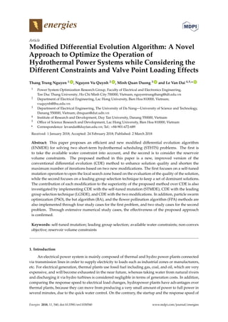
![Energies 2018, 11, 540 2 of 30
thermal plants to load changes is very slow. Therefore, thermal plants need to run continuously for
some hours once they start. Based on the advantages and disadvantages analyzed for thermal and
hydropower plants, it is clear that the coordination of thermal and hydropower plants in electrical
generation operations becomes more effective and economical. In summary, hydrothermal scheduling
(HTS) aims to minimize the electricity generation fuel cost of thermal plants using fossil fuels, while
all constraints from thermal plants, hydropower plants and the system are exactly met [1]. With regard
to this problem, the thermal power plant constraints are easily met, because only limitations on
generation are taken into consideration and other constraints such as fossil fuel constraints and fuel
costs for the start-up and shutdown processes are neglected. Among the optimization problems
related to the optimal scheduling of hydrothermal systems, the fixed-head, short-term HTS problem
has been widely and successfully studied so far [1–29]. The fixed-head, short-term HTS problem
has been classified into two sub-problems with different hydraulic constraints, namely the amount
of discharged water available via the turbine [1–17] and reservoir volume limits [2,3,18–34]. In the
two sub-problems, the water head of reservoirs is not supposed to be changed over the scheduled
time, thus the water discharge function of the two problems has the same quadratic function model
with respect to hydro generation and coefficients; however, the set of hydraulic constraints taken into
account in the problems are almost completely different. The water volume, which is allowed to run
the hydro turbines over the scheduled horizon, is constrained in the first problem, while the main
constraints considered in the second problem are the reservoir volume at the beginning and the end of
the scheduled horizon, the limitations of the reservoir volume and the water balance in each reservoir.
Several methods have been used to solve the first problem, such as Powell’s hybrid method [1]; the
Newton–Raphson method [1,2]; the lambda–gamma method (λ-γ method) [2]; the Lagrange-multiplier,
factorization-based, Newton–Raphson method [3]; the Lagrange method based on the linearization
of the coordination equation (LCEL) [4]; the Lagrangian relaxation approach [5]; Hopfield neural
networks (HNN) [6]; evolutionary programming (EP) [7,8]; the artificial immune system method
(AIS) [8]; particle swarm optimization (PSO) and the differential evolutionary method (DE) [8];
the modified bacterial foraging algorithm (MBFA) [9]; the optimal gamma-based genetic algorithm
(OGB-GA) [10]; fast genetic algorithm (FGA) [11]; the predator–prey optimization technique (PPO) [12];
improved genetic with multiplier updating (IGA-MU) [13]; real-coded genetic algorithm (RCGA) [14];
a Hopfield Lagrange network (HLN) [15]; an augmented Hopfield Lagrange network (ALHN) [15];
the Cuckoo search algorithm (CSA) [16,17]; and a modified cuckoo search algorithm (MCSA) [17].
On the other hand, there has also been a number of methods proposed to solve the second problem,
such as gradient search (GS) [2]; Newton’s method [3]; the simulated annealing approach (SA) [18];
evolutionary programming (EP) [19–21]; genetic algorithms (GA) [22]; fast EP (FEP) [23]; improved fast
EP (IFEP) [23]; hybrid EP (HEP) [24]; PSO [25]; the improved bacterial foraging algorithm (IBFA) [26];
self-organizing, hierarchical PSO [27]; running improved fast EP (RIFEP) [28]; improved PSO [29,30];
a clonal selection algorithm (CS) [31]; fully-informed particle swarm optimization (FIPSO) [32]; a
cuckoo search algorithm with Lévy distribution (CSA-Lévy) [33]; a cuckoo search algorithm with
Lévy Gaussian distribution (CSA-Gauss) [33]; a cuckoo search algorithm with Cauchy distribution
(CSA-Cauchy) [33]; a one rank cuckoo search algorithm with Lévy distribution (ORCSA-Lévy) [34];
and a one rank cuckoo search algorithm with Cauchy distribution (ORCSA-Cauchy) [34].
Among the introduced methods, the methods in [1–6,15] are in the family of deterministic
algorithms and the others in [7–14,16–34] are in the family of meta-heuristic algorithms. The first
method group is mainly based on the gradient to find the optimal solution. Meanwhile the second
method group searches for the optimal solution mainly based on the population. Moreover, the
methods in the first group are defined as derivative-based optimization methods, finding the
optimal solution by a single path search line and suffering from the drawback that they cannot
deal with non-convex problems where the objective functions or constraints of the problems are
non-differentiable or nonlinear. In addition, the conventional methods also suffer from difficulties when
dealing with large-scale problems with complicated constraints. On the contrary, the meta-heuristic](data:image/gif;base64,R0lGODlhAQABAIAAAAAAAP///yH5BAEAAAAALAAAAAABAAEAAAIBRAA7)