2. properties of each phase play a vital role in the efficiency of the flota-
tion process. Flotation process encompasses three important factors
involving ore features (e.g. mineralogy and degree of liberation), cell
hydrodynamics (e.g. air flowrate, cell geometry and agitation type) and
chemical reagents (e.g. collector, frother, modifier, activator and de-
pressant) to obtain desirable metallurgical outcomes (i.e. grade, re-
covery and selectivity index (SI)) (Hassanzadeh and Hasanzadeh,
2016).
From the microscopic point of view, the particle–bubble encounter
efficiency (Ec) which is predominantly controlled by hydrodynamic
forces can be considered as the most effective initial sub–process in
flotation rate constant. Estimation of the Ec and its modeling are gen-
erally performed using three different techniques viz. analytical, nu-
merical and experimental approaches. Each method has some restric-
tions leading to deviation of the measured and/or estimated values
from the actual amounts. Detailed insights in this regard are reported
elsewhere (Min et al., 2008; Hassanzadeh, 2018; Wang et al., 2018). In
the previous work, we found that direct experimental visualization of
the particle-bubble sub-processes is very complicated owing to the
difficulties in terms of isolating these microprocesses from each other in
an actual flotation separation system (Hassanzadeh et al., 2018a).
However, the fundamental deviations between analytical and numer-
ical approaches based on the applied models were not discussed for
specific case studies which are covered in this research work.
Apart from the particle-bubble interactions, flotation rate constant
(k) is a key factor for optimization and improvement of circuit flow-
sheets and scale-up principles (Reuter and van Deventer, 1992; Mesa
and Brito-Parada, 2018). Macroscopic modeling of rate constant was
extensively studied over the past decades which is now basically cate-
gorized in two empirical and phenomenological (population balance,
mathematical and probabilistic) models (Gharai and Venugopal, 2016;
Prakash et al., 2018). From the 1930′s to early 1990, various mathe-
matical and practical flotation kinetic models were proposed and ex-
amined under different flotation conditions (Zuniga, 1935; Kelsall,
1961; Arbiter and Harris, 1962; Imauzimi and Inoue, 1963; Woodburn,
1970; Jowett and Safvi, 1960; Trahar and Warren, 1976; Harris, 1978;
Klimpel, 1980; Agar et al., 1989; Mehrotra and Padmanabhan, 1990;
Kelly and Carlson, 1991; Ek, 1992; Yuan et al., 1996). Nevertheless, it is
now accepted that there is no unique flotation kinetic model applicable
to the froth flotation processes (Dowling et al., 1985; Nguyen and
Schulze, 2004). The majority of the empirical models have fitted
first–order kinetic models to the experimental data which are valid only
at steady–state conditions (Azizi et al., 2015; Albijanic et al., 2015; Ni,
et al., 2016; Hassanzadeh and Karakaş, 2017a). The inability of these
empirical and phenomenological models to describe the flotation rate
constant under various flotation conditions has made them unsuitable
for assessment, control and monitoring purposes. Additionally, these
models are suffered from overfitting as it has been reported in several
research studies (Bu et al., 2017; Sahoo et al., 2016; Hassanzadeh et al.,
2018b) and information criteria (IC) was recommended as a reliable
approach rather than using common regression methods due to the
consideration of number of model parameters and model complexities
(Hassanzadeh, 2017a; Sahoo et al., 2016). Therefore, it appears that the
first principle and fundamental analytical modeling of flotation rate
constant can provide a universal way of evaluating the flotation kinetics
with a distribution of particle floatabilities (Nguyen and Schulze,
2004).
Several factors such as particle size (Trahar, 1981; Agheli et al.,
2018), bubble diameter (Tao, 2004), percent solids (Azizi et al., 2015),
particle residence time distribution (Lelinski et al., 2002; Hassanzadeh,
2017b), angle of tangency (Firouzi et al., 2011), water chemistry
(Michaux et al., 2018), particle roughness (Guven and Celik, 2016),
Nomenclature
k flotation rate constant
Np number of particles per unit volume
Nb number of bubbles per unit volume
Zpb collision frequency
Ec particle-bubble encounter efficiency
Ea particle-bubble attachment efficiency
Es particle-bubble stability efficiency
dp particle size
db bubble size
Vp particle relative velocity
Vb bubble relative velocity
ε turbulence dissipation rate
θ contact angle
f fluid density
tind induction time
Gfr gas flow rate
Vcell volume of vessel
Jg superficial gas velocity
CD drag coefficient
liquid viscosity
ν kinematic viscosity
f constant value = 2.03
Fatt attachment force
Fdett detachment force
t time
p particle density
d32 Sauter mean diameter
a adhesion angle
Ib interfacial area of bubbles
NB nanobubble
K3 and β dimensionless numbers
Ec
GSE
generalized Sutherland equation
Ec
YL
Yoon–Luttrell collision model
Ec
SU
Sutherland equation
Ea
DF
modified Dobby–Finch model
Ea
YL
Yoon–Luttrell attachment model
Es
SC
modified Schulze stability model
Kst Stokes number
Reb bubble Reynolds number
Sb bubble surface area flux
λ micro–turbulence
Ec
AK
Afruns-Kitchner collision model
Cp particle circularity
BO Bond number
g gravitational constant
t angle of tangency
σ surface tension
MRTb mean bubble residence time
g gas hold-up
RTD residence time distribution
CCD central composite design
ANOVA analysis of variance
MLR multi linear regression
ANN artificial neural network
RSM response surface modeling
Ecoll collection efficiency
As empirical stabilization constant = 0.50
TKE total kinematic energy of turbulence
DF degree of freedom
DOE design of experimental
MB microbubble
A and B constants in attachment efficiency model
A. Hassanzadeh, et al. Minerals Engineering xxx (xxxx) xxxx
2
3. morphology (Verrelli et al., 2014), density (Shi and Fornasiero, 2009)
and particle terminal settling velocity (Nguyen et al., 1997), contact
angle (Chaua et al., 2009), bubble surface contamination (Malysa et al.,
2005), bubble velocity (Hassanzadeh et al., 2016), superficial gas ve-
locity and gas hold-up (Newcombe et al., 2013), rotor speed
(Newcombe et al., 2018) and power input (Safari et al., 2016), cell
aspect ratio (Tabosa et al., 2016), fluid flow regime (Kouachi et al.,
2015) and turbulent dispersion rate (Fallenius, 1987) play significant
roles in maximizing both Ec and k in the froth flotation processes. A
brief explanation describing the main effect of each parameter on Ec
and k is given below and schematically represented in Table 1.
Turbulence dissipation rate ( ): An optimum flotation rate constant
is essential not only to maximize the particle–bubble encounter effi-
ciency but also to minimize the particle–bubble detachment (Schubert,
2008). More specifically, the cell turbulence leads to a slight increase in
the flotation rate constant of fine and intermediate sizes of dense par-
ticles and in turn to an increase in particle–bubble collision frequency
(Zpb), production of smaller bubbles by breakup and volume of pulp that
sweeps through the bubble (Vpath). On the contrary, a substantial de-
crease in the flotation rate constant of coarse particles occurs due to a
decrease in the particle–bubble aggregate stability, particularly for
denser minerals.
Contact angle ( ): Particle contact angle leads to an increase in the
collection efficiency and flotation rate constant due to an increase in the
attachment efficiency (Najafi et al., 2008). Both static and dynamic
contact angles vary substantially as a function of mineral surface
roughness, heterogeneity together with particle shape and size prop-
erties (Chau et al., 2009). For a given particle size, there is a critical
contact angle below which particles do not attach to bubble interfaces;
contact angle increases with a decrease in particle size (Chipfunhu
et al., 2012). Meanwhile, the flotation rate constant increases rapidly
and slightly with an increase in contact angle of intermediate and
coarse size fractions, respectively (Muganda et al., 2011).
Percent solids (%S): There is an optimal pulp density where max-
imum k and Ec can be achieved in froth flotation. Increasing % solid
results in greater collision frequency, however, it negatively affects the
pulp rheology inducing an increase in entrainment of gangue minerals
in the froth zone. Furthermore, a high percent solids and/or attractive
interaction between fine particles can also increase the pulp viscosity
leading to a decrease in turbulent energy dissipation rate, which in turn
induces a negative effect on the Zpb (Fornasiero and Filippov, 2017).
Particle size (dp): There is a large amount of evidence indicating that
Ec increases with increasing the particle size. Fine particles have low
relative velocity and thus a lower collision probability with bubbles
compared with coarse particles. However, the behavior of k versus dp
follows different trends. As a general rule, k decreases gradually when
the range of particle size becomes finer due to an increase in the
number of particles per unit weight, the deteriorating conditions for
particle–bubble collision in connection with low mass and inertia, in-
sufficient kinetic energy for rupturing the thin water film in particle-
bubble interface and formation of three–phase line of contact (TPLC),
possessing lower critical contact angle than needed for flotation and
such effects as increasing surface oxidation of the particles. The k also
decreases suddenly above an optimum particle size either due to a low
degree of mineral liberation or reduced ability of bubbles to lift the
coarse particles (Trahar, 1981; Hassanzadeh and Karakas, 2017b).
Particle density ( p): It is believed that increasing particle density
enhances the Ec, however, numerical results reveal that there are two
distinct zones where the particle density plays completely different
roles. In the first zone, increasing particle density reduces the Ec,
whereas, in the second zone, increasing particle density leads to an
increase in the Ec (Liu and Schwarz, 2009). Increasing the particle
density at constant particle size, in general, reduces the flotation rate
constant (Shi and Fornasiero, 2009). There is a critical set of particle
diameter and its density where the collision angle is minimal (Nguyen
et al., 2006; Firouzi et al., 2011).
Angle of tangency ( t): The analytical results predict a continuous
decrease in the angle of tangency with increasing the particle size
(Kouachi et al., 2017). However, numerical outcomes indicate that
there is a critical particle size where the angle of tangency is minimal
(Firouzi et al., 2011).
Bubble size (db): A decrease in the bubble size increases the parti-
cle–bubble encounter and attachment efficiencies and in turn causes an
increase in the flotation rate and recovery of fine particles (Reay and
Ratcliff, 1973; Hassanzadeh et al., 2016). Therefore, enhancement of
flotation efficiency particularly in the range of fine (< 20 µm) and ul-
trafine (< 10 µm) particles using combination of conventional macro-
bubbles (1 mm < CMBs < 100 µm) with microbubbles (1 µm <
MBs < 100 µm) and nanobubbles (NBs < 1 µm) is one of the key
developments in this field (Temesgen et al., 2017). Small bubbles have
low relative velocities leading to a substantial increase in their numbers
at the same airflow rate, which brings an increase in the particle col-
lision probability in interaction with fine particles. However, if the
bubbles are too small, they cannot lift the particles to the quiescent
zone owing to insufficient buoyancy force. Increasing the bubble size at
a constant bubble velocity results in an increase in the flotation rate
constant of coarse particles but leads to a decrease in the flotation rate
constant of fine particles (Pyke, 2003).
Bubble velocity (vb): Increasing bubble velocity above a threshold
decreases the Ec due to a decrease in the maximum possible collision
angle and likewise, k is reduced owing to a reduction in the attachment
efficiency (Pyke, 2003). Addition of frother reduces bubble rise velocity
which depends on the type and dosage of the frother.
It is known that the flotation process is affected by many interlinked
factors. For instance, changing the db impacts significantly on the vb
(Ghatage et al., 2013) and varying surface contamination of the bubble
is highly effective on bubble diameter and bubble velocity (Laskowski
et al., 2008; Kulkarani and Joshi, 2005; Rafiei Mehrabadi, 2009). Also,
turbulence has a major effect on db (Amini et al., 2013) and vb (Nesset
et al., 2006) in a flotation cell. Bubble size and shape can also be in-
fluenced by solids concentration (Rocha et al., 2008; Finch et al., 2008;
Vazirizadeh, 2015). Bubbles become smaller in the presence of fine
particles (air-water-solid system) than that in the absence of them (air-
water system) (Hoang et al., 2019) due to inhibiting bubble coalescence
and forming larger bubbles. Further, bubbles become more rounded as
the %S increases and the dp decreases (Rocha et al., 2008). Moreover,
the interaction of air flow rate and froth thickness (pulp level) induces a
significant effect on flotation rate constant (Cilek, 2004). Particle re-
sidence time distribution (RTD) and its measurement are impacted by
slurry density and particle density (Newcombe et al., 2013). The in-
terrelated relation of gas hold–up, the interfacial area of bubbles and
bubble surface area flux significantly affect k (Vazirizadeh et al., 2015).
Therefore, it is not preferred to use one–factor at a time (OFAT) method
due to neglecting the interaction effects of the factors. Despite a wide
Table 1
A schematic summary on the impact of key hydrodynamic factors on the Ec and k.
Parameter (m2
/s3
) (˚) %S (%) dp(µm) p(g/cm3
) t(˚) db(cm) vb(cm/s)
Ec (%) ↑ ↑ ↑ ↑ ↑↓ ↑↓ ↓ ↓
k (1/min) ↑↓ ↑ ↑↓ ↑↓ ↓ ↑↓ ↓ ↓
A. Hassanzadeh, et al. Minerals Engineering xxx (xxxx) xxxx
3
4. series of scientific researches on kinetic behavior of flotation and the
particle-bubble collision interactions, the relative intensity of main
flotation parameters on the particle–bubble interactions together with
their interrelations has not been adequately investigated. The effects of
key parameters on Ec and k are less explored in the absence and pre-
sence of cell turbulence. Less attention has been given to evaluate the
simultaneous effects of important variables. On the other hand, the
complication of the flotation mechanism and the interdependence of
the effective factors usually make the quantitative and predictive
modeling much more difficult.
Over the last three decades, in terms of inability in physical ob-
servations of microscopic phenomena, the two most common techni-
ques in flotation modeling were numerical and analytical approaches to
study the flotation system in actual conditions. Therefore, the initial
aim of the present study is to evaluate and analyze two most common
model configurations (i.e. (Ec
GSE
, Ea
DF
and Es
SC
) and (Ec
YL
, Ea
YL
and Es
SC
))
used for estimating the particle–bubble collection efficiencies in ana-
lytical and numerical studies while five crucial parameters in flotation
are varied. Following the first aim, the second purpose is to identify the
main and interactive significant factors as well as their order on esti-
mation and optimization of the Ec and k. The central composite design
(CCD) method is introduced as an efficient approach to cope with this
difficulty in connection with finding a suitable modeling method to
predict the particle–bubble encounter probability and flotation rate
constant.
2. Theory and methodology
Several thermodynamic and kinetic-based approaches were pre-
sented in the last century of flotation modeling with the aim of pre-
dicting the rate constant which was summarized in detail by Massey
(2011). In the present study, the most common flotation kinetic equa-
tion (Eq. (1)) was used (Pyke et al., 2003; Duan et al., 2003; Chipfunhu
et al., 2012; Govender et al., 2013; Karimi et al., 2014 a, 2014b; Popli
et al., 2015). It was initially proposed by Ahmed and Jameson (1989)
based on the assumptions that the reaction is first–order, bubble con-
centration in the pulp is constant, and the volume of particles removed
is negligible. According to Derjaguin and Dukhin (1993), the collection
efficiency (Ecoll, so–called capture efficiency, Ecap) was calculated as the
product of three probability functions (Ec.Ea.Es), well-known as three-
zone model, quantifying the collision, attachment, and detachment
(stability) efficiencies presuming that sub-processes are independent of
each other, particle diameters are smaller than bubble sizes and parti-
cles and bubbles are spherical.
= =
dN
dt
kN Z E E E
p
p pb c a s
(1)
where t (s) is time, Np the number of particles and k (1/s) the flotation
rate constant. Ec, Ea and Es were consecutive sub–processes comprising
the particle–bubble collision, attachment and stability. Zpb (m3
/s) is the
collision frequency per unit volume between particles and bubbles of
diameters dp and db (m), respectively.
Table 2
Classification of previous works in two groups incorporated two fundamental modeling configurations for prediction of Ecoll.
Author(s) Year Notes
Configuration I (E E E
and
,
c a
DF
s
SC
GSE
) Dai et al., 1998 A good agreement between experimental and calculated collection efficiencies of angular and
smooth quartz particles was reported using single particle-bubble interaction by assuming unity for
Es.
Pyke et al., 2003 and
2004
Agreement between the GFK model and experimental data given by floating methylated quartz,
chalcopyrite and galena particles in Smith-Partidge and Rushton flotation cells was satisfactory,
depending upon the mineral and particle size involved.
Duan et al., 2003 k-values of chalcopyrite in a complex sulfide ore floated in a Rushton flotation cell were found in a
good agreement with calculated k-values
Newell 2006 Computed-k for different minerals validated the analytical computations using the experimental
measurements of the flotation rate constants.
Ralston et al., 2007 Industrial data taken from rougher flotation stage of an operating plant using a property-based
model approach was shown.
Kouachi et al., 2010 Analytical approach was applied for calculating k-values of quartz, chalcopyrite and galena using
GFKM while , Reb, db, and vb varied in specific intervals demonstrating the impact of particle
inertial forces.
Karimi et al., 2014a The numerical (CFD) predictions were validated against experimental data on quartz particles and
analytical computations using the fundamental flotation model of Pyke et al. (2003) under different
ranges of hydrophobicity, agitation speed and gas flow rates.
Karimi et al., 2014b Qualitative and quantitative agreements between k-values obtained by developed CFD-kinetic
model and experimental data (Pyke et al., 2003) for chalcopyrite and galena in the same physical
setup were reported.
Kouachi et al., 2017 Three minerals i.e. quartz, chalcopyrite and galena were used to study the role of particle density
and particularly particle’s inertial effect on particle-bubble interactions and flotation rate constant.
Configuration II (E E E
and
,
c
YL
a
YL
s
SC
) Koh and Schwarz 2003 CFD of a CSIRO flotation cell was performed using an Eulerian–Eulerian approach for particle sizes
7.5, 15, 30 and 60 µm at 800, 1000 and 1200 rpm stirring speeds. Collection rates were found
greater than observed flotation rates.
Koh and Schwarz 2006 The flotation kinetic rates were obtained using CFD technique in a semi-batch process (3.78L) via a
multi-phase flow equations and an Eulerian–Eulerian approach.
Koh and Schwarz 2007 Flotation kinetics in a Denver laboratory cell was studied using CFD modelling at various impeller
speeds. Correlating the results with the literature data for quartz (Ahmed and Jameson, 1985)
showed reasonable agreements in the presence of buoyancy reduction factor.
Evans et al., 2008 It was reported that simulation results obtained for a Rushton turbine were fairly in good agreement
with the practical results presented by Ahmed and Jameson, 1985.
Govender et al., 2012 The multiphase CFD model developed by Ragab and Fayed (2012) was utilizes and applied to two
industrial case studies of porphyry copper rougher-scavenger flowsheets comprised of Wemco and
Dorr-Oliver machines operating in high and low rpms. Surprisingly, extremely large numbers for
pseud k-values (0 < k < 300 min−1
) were reported.
Schwarz et al., 2016 A sequential multi-scale modelling approach using multi-phase CFD models were applied to large-
scale flotation cells.
Zhou et al., 2019 Pure pyrite samples were floated by means of a micro-flotation column focusing on induction time
and flotation rate constant.
A. Hassanzadeh, et al. Minerals Engineering xxx (xxxx) xxxx
4
5. To calculate Zpb, several formulas were presented by Smoluchowski
(1917), Camp and Stein (1943), Saffman and Turner (1956), and
Abrahamson (1975) which were discussed in detail elsewhere
(Hassanzadeh et al., 2018a). Abrahamson (1975)’s model (Eq. (2)),
well–accepted for the flotation processes (Schubert, 1999; Koh et al.,
2000; Liu and Schwarz, 2009), was used in this study. According to
assumptions of Abrahamson’s model (i.e. highly turbulent condition
and infinite Stokes number), the Ec is approximately 1. However, in an
actual flotation condition, as the turbulent is not infinitive, the use of
collision efficiency model provides much less value in serving as a
correction factor for Zpb (Sherrell, 2004).
=
+
+
Z N N
d d
V V
5 (
2
) ( )
pb p b
p b
p b
2
2 2
(2)
where Np and Nb were the number of particles and bubbles per unit
volume, Vp and Vb (m/s) were turbulent root–mean square (RMS) ve-
locities of particle and bubble relative to the turbulent fluid velocity
which could be approximated by the following expression (Eq. (3))
(Schubert and Bischofberger, 1978; Schubert,1999):
V
d
v
( ) 0.33 ( )
i
i p f
f
2
1/2
4
9
7
9
1
3
2
3
(3)
where the subscript i refers to the particle or bubble, (W/kg) denotes
the dispersion rate of the turbulent kinetic energy per unit mass, v (m2
/
s) is the kinematic viscosity of the fluid, p and f (kg/m3
) are particle
and fluid densities, respectively.
By combining Eqs. (1) and (2), it could be shown that;
=
k N
d d
v
E E E
5
4
[0.33 ]
b
b b p f
f
c a s
2 4
9
7
9
1
3
2
3
(4)
where Nb represented by gas flow rate Gfr (cm3
/min) and bubble re-
sidence time, MRTb (min), per unit volume of a vessel (Vcell).
By assuming that db > > dp (which is broadly verified) (Chipfunhu
et al., 2012), Eq. (5) can be eventually shown as:
=
k
G
d V
d
v v
E E E
2.39 [0.33
1
]
fr
b cell
b p f
f b
c a s
4
9
7
9
1
3
2
3
(5)
The capability of Eq. (5) was experimentally examined for the flo-
tation of quartz, chalcopyrite and galena in several studies (Pyke et al.,
2003; Pyke, 2004; Duan et al., 2003; Newell, 2006; Newell and Garno,
2006). Additionally, Karimi et al. (2014a, 2014b) presented a good
agreement between the experimental and numerical data on the flota-
tion of quartz, chalcopyrite and galena using computational fluid dy-
namics (CFD) under various contact angles, agitation and gas flow
rates. More importantly, it was validated by industrial data taken from
the rougher flotation stage of an operating plant using a property-based
model approach (Ralston et al., 2007). Therefore, the agreement of
experimental, numerical and industrial results with the theoretical
model of Eq. (5) was led us to confidentially calculate the flotation rate
constants.
Two most widely used model configurations to obtain the Ecoll are
examined in the following section.
2.1. Selection of two model configurations
As noted in Eq. (5), the most crucial term is estimation of
Ecoll = Ec × Ea × Es by presuming that (i) sub-processes are in-
dependent of each other (ii) particles and bubbles are spherical (iii)
particles are finer than bubbles (iv) flow around the bubble is modeled
as if the bubbles are stationary in a flow field giving the equivalent
bubble rise velocity and (v) only one particle interacts with each
bubble.
Considering the existing analytical models of the collision,
attachment and detachment, the two most common model configura-
tions were selected as follows:
(I) Dukhin so–called generalized Sutherland equation (Ec
GSE
), modified
Dobby–Finch attachment (Ea
DF
) and modified Schulze stability
(Es
SC
) models (i.e. (Ec
GSE
, Ea
DF
, Es
SC
) and,
(II) Yoon–Luttrell (Ec
YL
), Yoon–Luttrell (intermediate) (Ea
YL
) and mod-
ified Schulze stability (Es
SC
) models (i.e. (Ec
YL
, Ea
YL
, Es
SC
)).
For more than two decades, these two model configurations have
been utilized for estimating the Ecoll and k. One school of mind has used
configuration I (mostly in analytical works) and the other made use of
configuration II (numerical studies) for prediction of Ecoll and k values
as shown in Table 2. However, to the best of the authors’ knowledge,
the discrepancy of these configurations has not been discussed at all in
the literature which is addressed in the first phase of this present work.
The following briefly expresses concepts and assumptions in con-
nection with Ec
GSE
vs. Ec
YL
as for collision well as Ea
DF
vs. Ea
YL
for at-
tachment.
Dukhin (1983) collision model (so–called Ec
GSE
) was experimentally
verified and used by Dai (1998), Pyke (2003), Sherrell (2004), Duan
et al. (2003), Newell (2006) and Miettinen (2007). However, recent
numerical studies demonstrated its inaccuracy due to poor estimation
of the collision angle and disregarding the microhydrodynamics and
bubble wall effects (Phan et al., 2003; Liu and Schwarz, 2009; Firouzi
et al., 2011). On the other hand, the collision model developed by Yoon
and Luttrell (1989) (Ec
YL
) was accepted as an accurate model and used
by several researchers (Koh and Schwarz, 2006; Evans et al., 2008;
Shahbazi et al., 2009; Jamson 2010; Govender et al., 2013; Yoon et al.,
2016; Hoang et al., 2018; Zhou et al., 2019). They applied the inter-
ception mechanism and an empirical stream function valid for inter-
mediate flow conditions where the bubble Reynolds number is between
1 and 100. However, it was only applicable to particles finer than
100 µm and bubbles smaller than 1 mm with immobile surfaces which
did not cover particle and bubble ranges in flotation conditions.
The Ec
YL
(Eq. (6)) and Ec
GSE
(Eq. (7)) were selected to estimate the
Ecs.
= +
E
Re R
R
(
3
2
4
15
)( )
c
b p
b
YL
0.72
2
(6)
where Reb is bubble Reynolds number, Rp and Rb indicate particle and
bubble radii, respectively.
= ×
+
E E sin exp K cos ln
E
K cos
E sin
3
3
1.8
9 ( )
2
c
GSE
c
SU
t t
c
SU
cos
t
c
SU
t
2
3
3
2
3 3
2
t
3
(7)
where Ec
SU
represented Sutherland collision model ( =
Ec
SU d
d
3 P
B
), tin
degree referred to the angle of tangency (Eq. (8)) (maximum collision
angle) which was described as the angle above which no encounter was
possible and K3 was given by Eq. (9).
= +
arcsin(2 ( 1 ))
t
2 1/2
(8)
= =
K K
v
d
( ) 4 ( )
9
st
p f
p
b p f
b
3
(9)
where the Kst term represents the particle Stokes number as =
Kst
v d
d
9
p b p
b
2
and being the liquid viscosity. Dimensionless number was calcu-
lated by Eq. (10).
=
fE
K
2
9
c
SU
3 (10)
A. Hassanzadeh, et al. Minerals Engineering xxx (xxxx) xxxx
5
6. where f is a constant value equal to 2.034 (Dukhin and Rulyov, 1977).
Basically, Ea depends upon the surface characteristics of the mineral
and the degree of collector adsorption on the mineral surface (Albijanic
et al., 2010; Xing et al., 2017). Attachment efficiencies measured in
several studies (Dai, 1998; Duan et al., 2003; Pyke et al., 2003) aimed
to test the particle–bubble attachment model showed good agreement
with those predicted using the modified Dobby and Finch attachment
efficiency model (Ea
DF
) (Dobby and Finch, 1987). Likewise, other re-
searchers used Ea
DF
in their studies (Dai et al., 2000; Pyke, 2004;
Newell, 2006; Karimi et al., 2014a; Hassanzadeh et al., 2016; Kouachi
et al., 2017; Popli, 2017). Similarly, Yoon–Luttrell attachment model
(Ea
YL
) was utilized for the estimation of Ea in several studies (Koh and
Schwarz, 2003, 2006; 2007; Evans et al., 2008; Govender et al., 2013;
Schwarz et al., 2016; Yoon et al., 2016; Zhou et al., 2019). More de-
tailed information concerning both Ea
YL
and Ea
DF
can be found elsewhere
(Kouachi et al., 2010).
Thus, Ea
YL
(Eq. (11)) Yoon–Luttrell (1989) and Ea
DF
(Dobby and
Finch, 1987) (Eq. (12)) were selected to calculate the Ea;
=
×
+
+
E
sin
sin
(2 arctan(exp[ ]))
90
a
YL
v t Re
d d d
2
(45 8
15 ( / ( 1))
2
b ind b
b b p
0.72
(11)
where tind (s) is induction time described in detail elsewhere (Dai et al.,
1999)
=
E
sin
sin
a
a
t
2
2 (12)
where a the adhesion angle in (°), was the specific collision angle
where its sliding time being equal to the induction time. The a was the
collision angle where sliding time equaled its induction time (tind):
=
+ +
+
+
( )
arctanexp t
v v v
d d
2
2( ) ( )
a ind
P b b
d
d d
p b
3
b
p b
(13)
The induction time calculated using Eq. (14).
=
t Ad
ind p
B
(14)
where B was constant and independent of the particle size ( 0.6 ± 0.1)
(Duan et al., 2003) and A was inversely proportional to the particle
contact angle (Dai et al., 1999).
Modified Schulze (1992) stability model was chosen for determining
detachment efficiency of particle–bubble as below:
= =
E A
F
F
A
B
1 exp 1 1 exp 1
1
stab s
att
det
s
O (15)
where As was a constant value of 0.5 (Bloom and Heindel, 2002;
Govender et al., 2013). The ratio of the detachment force (Fdet) to the
attachment force (Fatt) was a dimensionless term indicated as Bond
number (B )
O by Eq. (16) (Pyke et al., 2003; Koh and Schwarz, 2007).
=
+ + +
+
( )
( )
B
d g d d p g sin
( ) 1.9 1.5 ( ) ( )
6 sin sin( )
O
p p f p
d d
p d b f
2
2 2
4 2
2
2 2
p b
b
2
3
1
3
(16)
where (°) was the contact angle, (N/m) surface tension, g (m/s2
)
gravitational constant and (W/kg) was energy input.
The power value of each parameter in Eq. (16) was experimentally
examined by Safari and Deglon (2018) with the aim of proposing a new
attachment–detachment flotation kinetic model.
As a general rule, particle size fractions in the range of 1–100 µm
were selected in this study to cover fine (< 20 µm), middling or in-
termediate (20–75 µm) and coarse (75–100 µm) fraction sizes (Trahar,
1981; Feng and Aldrich, 1999). Depending on the reagent type and
dosages, impeller speed and other relevant operating factors, bubble
size and its velocity were considered in the typical range of
0.05–0.10 cm (Tao, 2004; Grau and Heiskanen, 2005; Laskowski et al.,
2008) and 10–30 cm/s (Kowalczuk et al., 2017), respectively. Particle
density was considered < 4.1 g/cm3
since the large discrepancies be-
tween models and experimental data were found mostly for the flota-
tion of dense minerals, e.g. galena (Pyke, 2004; Safari and Deglon,
2018; Kouachi et al., 2017; Pyke, 2004). Contact angle of the materials
were considered 75° for p = 2.7 g/cm3
(e.g. quartz) (Miettinen, 2007;
Guven et al., 2015), 62° for p = 1.3 g/cm3
(e.g. coal) (He et al., 2018),
56° for p = 4.1 g/cm3
(e.g. chalcopyrite) (Pyke et al., 2003; Abreu
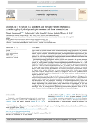
Fig. 1. A comparison between the particle-bubble interactions using two model configurations: (a) encounter (Dukhin (GSE) vs. Yoon-Luttrell (YL)), (b) attachment
(Dobby-Finch (DF) vs. Yoon-Luttrell (YL)) and (c) configuration I vs. configuration II.
A. Hassanzadeh, et al. Minerals Engineering xxx (xxxx) xxxx
6
7. et al., 2010), 68° for p = 3.4 g/cm3
(e.g. apatite) (Zhou et al., 2015),
62° for p = 2.0 g/cm3
(e.g. Trona) (Ozdemir et al., 2009) to cover the
values greater than the critical contact angles. Turbulence dissipation
rate was given in the range of 18–30 m2
/s3
in order to provide intensive
turbulence system in a Rushton turbine cell as described by Pyke (2004)
and Duan et al. (2003). The rest of the parameters were kept constant as
gas flow rate of 3500 cm3
/min, liquid viscosity of 0.00891 g/cms, water
surface tension of 72dyne/cm, the fluid density of 0.997 g/cm3
and
kinematic viscosity of 0.0089 cm2
/s as detailed by Pyke (2004).
3. Optimization technique–response surface method (RSM)
Design of experimental (DOE) methodology was used to incorporate
the interaction effects into the modeling technique. The response sur-
face methodology (RSM), a well–known statistical technique (Box and
Wilson, 1951; Box and Hunter, 1957; Martinez–L et al., 2003; Kalyani
et al., 2005; Dashti and Eskandari Nasab, 2013), was utilized for
modeling and optimization of the flotation process. In this regard,
second–order models were applied as they provide a high degree of
flexibility and applicability in a wide variety of functional forms. These
advantages lead to a good approximation of the true response surface.
Also, it is very easy to estimate the parameters in a second–order model
using the method of least squares.
To determine a critical point (maximum, minimum, or saddle), it is
necessary for the polynomial function to contain quadratic terms ac-
cording to the following equation:
= + + +
= < < < <
Y x x x x
i
k
i i
i j
k
ii i
i j
k
ij i j
0 1
2
1 (17)
where k, 0, i, xi, ii, ij and represent number of variables, constant
term, coefficients of the linear parameters, variables, coefficients of the
quadratic parameters, coefficient of the interaction parameters and
residual associated to the experiments, respectively (Bezera et al., 2008;
Mehrabani et al., 2010).
Finally, the codes were calculated as functions of the range of in-
terest of each factor. A detailed discretion in this regard can be found
elsewhere (Azizi et al., 2012).
4. Results and discussions
4.1. Estimation of Ec, Ea and Ecoll
Fig. 1 displays the particle–bubble interaction probabilities for 30
runs. Fig. 1a shows the differences between the particle–bubble en-
counter efficiencies using Ec
GSE
and Ec
YL
models. Fig. 1b presents the
values given by modified Ea
DF
and Ea
YL
(intermediate) attachment
models. Also, Fig. 1c indicates the particle–bubble collection effi-
ciencies using two types of model configurations (i.e. (Ec
GSE
, Ea
DF
and
Es
SC
) and (Ec
YL
, Ea
YL
and Es
SC
)).
It can be seen in Fig. 1a that Ec
YL
and Ec
GSE
have relatively similar
trends. However, it can be found that Ec
YL
is much more dependent on
particle diameter thanEc
GSE
. The minimum and maximum Ecs for Ec
YL
occur when the particle size is respectively coarser than 78 µm (runs 13,
21, and 25) and finer than 33 µm (runs 8, 12, 14, 20, and 23) regardless
of the values of other factors. However, it appears that the Ec
GSE
takes
the combination of the factors into account. In this regard, Schulze
(1989) and Dai et al. (1998) noted that the assumptions involved in
predicting Ec
YL
are unrealistic. Following this, Dai et al. (2000) com-
pared experimental and predicted encounter efficiencies for several
models in a specific flotation condition (dp < 70 µm, db = 0.08 and
0.15 cm, vb = 31.60 and 19.60 cm/s and p = 2.65 g/cm3
) assuming
that the particle–bubble stability is equal to unity. It was pointed out
that Ec
YL
underestimates Ec in comparison with Ec
GSE
due to ignoring the
particle inertial forces and assuming a uniform distribution of collision
over the entire upper half surface of the bubble; this is in a relatively
good agreement with our findings. Also, King (2001) indicated the
dependence of theoretical and experimental collision efficiencies on
different bubble (0–1.2 mm) and particle (12, 18, 27, 31 and 41 µm)
sizes. For theoretical estimations, Ec
YL
and Anfruns and Kitchener
(1977) (Ec
AK
) collision models were used for coal and quartz, respec-
tively. It was concluded that theoretical predictions overestimate Ec by
a factor of about two for bubbles approaching 1 mm in diameter. Most
recently, Darabi et al. (2019) applied Nguyen and Schulz, Ec
YL
(inter-
mediate I and II), and Schulze collision models to estimate overall Ec
values in an aerated mechanical flotation cell (10.5L) as a function of
particle size and superficial gas velocity (Jg). It was reported that for
coarse particles, Ec
YL
increased more sharply than the other models
which further confirms the presented results (e.g. runs 13, 21 and 25).
As shown by Fig. 1b, except for a few runs (3, 6, 13, 18, 21 and 25)
Ea
YL
varies very slightly in the vicinity of one. In other words, the es-
timated value of the Ea using Ea
YL
does not change upon varying the
effective factors. However, Ea
DF
shows different values as a function of
30 runs. In this regard, Shahbazi et al. (2009) used Ea
YL
for predicting
particle–bubble attachment probability of quartz in a mechanical flo-
tation cell and reported that the results were approximately zero for all
experiments. Kouachi et al. (2010) analyzed the Ec
YL
and Ea
YL
under
various flotation conditions for quartz and galena minerals. It was re-
ported that a large maximum collision angle (90 °
 ) used in the
Yoon–Luttrell model resulted in small attachment efficiencies. Newell
(2006) and Miettinen (2007) proposed a new attachment model (1/W
attachment model) based on the ratio between the rate of interaction
force controlled interparticle collision with and without electrostatic
double layer repulsion. Experimental attachment efficiencies compared
with corresponding values of 1/W attachment model, Yoon and Mao
model (Ea
YM
) and Ea
DF
. It was disclosed that Ea
DF
and 1/W attachment
model agreed with the experimental findings contrary to Ea
YM
which
showed an entirely opposite behavior.
Finally, it is found in Fig. 1c that the Ecoll estimated by applying the
configuration II gives greater values than that of using configuration I.
It implies that the numerical approach overestimates the Ecoll. In this
regard, Koh and Schwarz (2003) admitted that the collection rates
obtained by CFD approach were fast in comparison to the flotation rates
generally observed in either batch or plant-scale cells. Surprisingly, the
results of Govender et al. (2013) extremely overestimated k-values for
two case studies which are in complete disagreement with reported
results by Pyke et al. (2003), Karimi et al. (2014b), Jameson (2012),
Kouachi et al. (2017), Safari and Deglon (2018) and Jameson (2010)
who considered k-maximum < 10 min−1
. Therefore, according to the
data given in the literature (Table 2) together with the results obtained
from Fig. 1, the configuration I was chosen for the calculation of Ecap in
Eq. (5) to optimize k-values by evaluating five effective factors.
4.2. Estimation, order and interrelation of effective parameters on Ec
A series of 30 tests with appropriate combinations of particle size
(A), particle density (B), bubble size (C) and bubble velocity (D) were
conducted using the central composite design method. The design
matrix of these variables in coded units is given in Table 3 along with
the predicted values of the response (Ec). The factors were studied with
their codified values to simplify the calculations and for uniform
comparison. The factors are coded according to the following equation:
=
x
X X
X
i
i 0
(18)
where xi is the dimensionless coded value of the ith factor, Xi is the
actual value of the factor, X0 is the value of Xi at the center point and ΔX
is the step change value.
In order to describe the effect of factors on Ec, it is first necessary to
choose a suitable empirical model. Therefore, experimental data in
Table 3 were fitted to a full quadratic second order model equation by
applying multiple regression analysis for Ec using Design Expert soft-
ware (Demo v. 7.0.0, Stat–Ease, Inc.). Consequently, the final equation
A. Hassanzadeh, et al. Minerals Engineering xxx (xxxx) xxxx
7
8. (Eq. A(1), Table A.1) representing the Ec in terms of coded factors after
removing insignificant terms was obtained as shown in Appendix A.
Evidently, the regression coefficients of all four factors together
with interactions of the AB (dp and p) and BC ( pand db) terms were
found to be significant. The analysis of variance (ANOVA) was also
applied to estimate the adequacy of the model and its significance at the
95% confidence level. The coefficient of determination (R2
) was found
to be 0.97, which means that the model could explain 97% of the total
variations in the system. The p–value was found < 0.0001 indicating
the significance of the model due to being smaller than 0.05.
Fig. 2 shows the perturbation plot of the effects of the main factors
on the Ec, which is simulated from model fitting (Eq. A(1), Appendix A).
This plot helps to compare the effect of all the factors at a particular
point in the design space. A steep slope or curvature in a factor displays
whether the efficiency is sensitive to that particular factor. In addition,
3D response surface plots were applied to gain a better understanding
of the influence of factors and their interactive effects. Fig. 3 displays
the response surface plots of the effect of four factors on the parti-
cle–bubble collision efficiency.
Figs. 2 and 3 show that the order of significance of the studied
factors is as particle size, particle density, bubble diameter, and bubble
velocity (dp > p > db > vb). In other words, particle size positively
affects Ec the most whereas p, db and vb influence negatively under the
studied flotation conditions. The following contains a brief explanation
concerning the impact of each parameter along with a discussion with
the reported works in the literature.
The effect of dp has been extensively illustrated in the literature; the
Ec increases with increasing the particle size particularly in quiescent
conditions due to interceptional, gravitational and inertial forces
(Schulze, 1989; Dai et al., 2000; Ralston et al., 2002; Hassanzadeh
et al., 2018a). However, fine particles have extremely low affinity to
collide with bubbles because of low mass ratios leading to following the
surrounded streamlines around bubbles and eventually obtain poor Ec-
values. One possible solution is to aggregate fine particles to act as if
coarse particles which indeed opens up new avenues to research studies
on the floc-flotation for floating fine and ultrafine particles in future. In
this context, Safari et al. (2016) estimated k-values of three sulfide and
oxide minerals using oscillating grid flotation cell (OGC). It was re-
ported that the energy/power input as a key factor in flotation led to an
increase in the flotation rate for fine particles, an optimum k for more
moderate particles and a reduction in the flotation rate for coarse
particles. Nevertheless, Tabosa et al. (2016) indicated that the size of
turbulence zone is the main factor affects flotation recovery than the
energy input.
As reported in several studies (Reay and Ratcliff, 1973; Ahmed and
Jameson, 1985; Dobby and Finch, 1987; Tao, 2004), small bubbles (i.e.
MBs or NBs) enhance the Ec specifically in the case of fine particles. A
minimum improvement of ca. 10% in recovering coal, quartz (Nazari
et al., 2019), phosphate and rare earth elements (REEs) were reported
in the presence of an appropriate combination of macro-, micro- and
nano-bubbles. For instance, Pan et al. (2012) reported that the use of
MBs was more effective for increasing the kinetics of film thinning and
hence the flotation rate. The reason is attributed to long residence and
interaction time, high specific surface area and efficient mass transfer.
A detailed study on the effect of db and vb is given elsewhere
(Hassanzadeh et al., 2016) by exampling chalcopyrite’s flotation.
In this regard, Eskanlou et al., 2018) conducted experimental trials
and estimated the Ecs for pyrite and chalcopyrite using multiple linear
regression (MLR) and artificial neural network (ANN) techniques with
the aim of studying the impact of bubble surface area flux (Sb), micro-
turbulence ( ), particle circularity (Cp), bubble Reynolds number (Reb),
particle size (dp) and particle density ( p). The most influential factors
on Ec were introduced as Sb, Reb and dp. However, it could be found that
CP had a stronger impact on Ec than , dp and p. Other than that,
negatively influenced Ec which is in a complete disagreement with
fundamental concepts of the particle–bubble interaction (Duan et al.,
2003; Pyke et al., 2003; Govender et al., 2013; Cheng et al., 2017).
Generally, the influence of p and bubble rising velocity can be
discussed by two dimensionless numbers as Stokes ( =
Kst
v d
d
9
p b p
b
2
) and
bubble Reynolds ( =
Reb
v d
b f b
) numbers. The KSt is used to characterize
the behavior of particles suspended in a fluid flow. It is defined as the
ratio of the characteristic time of a particle to a characteristic time of
the flow. A particle with a low Stokes number (KSt < < 1) follows fluid
Table 3
Central composite design with actual/coded values for the parameters and re-
sults of the Ec.
Run Particle size
(dp) (µm)
(A)
Particle
density ( p)
(g/cm3
) (B)
Bubble size
(db)(cm)
(C)
Bubble
velocity (vb)
(cm/s) (D)
Collision
efficiency (Ec)
1 55 (0) 4.10 (2) 0.08 (0) 20 (0) 0.07
2 78 (1) 3.40 (1) 0.09 (1) 15 (−1) 0.08
3 78 (1) 3.40 (1) 0.09 (1) 25 (1) 0.08
4 55 (0) 2.70 (0) 0.08 (0) 20 (0) 0.08
5 33 (−1) 3.40 (1) 0.06 (−1) 15 (−1) 0.07
6 78 (1) 3.40 (1) 0.06 (−1) 15 (−1) 0.11
7 55 (0) 1.30 (−2) 0.08 (0) 20 (0) 0.15
8 33 (−1) 2.00 (−1) 0.09 (1) 15 (−1) 0.07
9 55 (0) 2.70 (0) 0.08 (0) 20 (0) 0.08
10 55 (0) 2.70 (0) 0.10 (2) 20 (0) 0.06
11 33 (−1) 3.40 (1) 0.06 (−1) 25 (1) 0.06
12 33 (−1) 3.40 (1) 0.09 (1) 25 (1) 0.04
13 78 (1) 2.00 (−1) 0.06 (−1) 25 (1) 0.13
14 33 (−1) 2.00 (−1) 0.09 (1) 25 (1) 0.06
15 55 (0) 2.70 (0) 0.08 (0) 20 (0) 0.08
16 55 (0) 2.70 (0) 0.08 (0) 10 (−2) 0.10
17 78 (1) 2.00 (−1) 0.06 (−1) 15 (−1) 0.17
18 78 (1) 2.00 (−1) 0.09 (1) 25 (1) 0.10
19 78 (1) 2.00 (−1) 0.09 (1) 15 (−1) 0.12
20 10 (−2) 2.70 (0) 0.08 (0) 20 (0) 0.03
21 100 (2) 2.70 (0) 0.08 (0) 20 (0) 0.10
22 55 (0) 2.70 (0) 0.08 (0) 20 (0) 0.08
23 33 (−1) 3.40 (1) 0.09 (1) 15 (−1) 0.05
24 55 (0) 2.70 (0) 0.08 (0) 20 (0) 0.08
25 78 (1) 3.40 (1) 0.06 (−1) 25 (1) 0.09
26 33 (−1) 2.00 (−1) 0.06 (−1) 25 (1) 0.09
27 55 (0) 2.70 (0) 0.08 (0) 20 (0) 0.08
28 33 (−1) 2.00 (−1) 0.06 (−1) 15 (−1) 0.10
29 55 (0) 2.70 (0) 0.08 (0) 30 (2) 0.07
30 55 (0) 2.70 (0) 0.05 (−2) 20 (0) 0.12
Fig. 2. Perturbation plot showing the relative significance of factors on the Ec.
A. Hassanzadeh, et al. Minerals Engineering xxx (xxxx) xxxx
8
9. streamlines and inertial forces have practically no effect on the motion
of the particle. However, a particle with a large Stokes number
(KSt > > 1) is dominated by its inertia and continues along its initial
trajectory. The Reb is generally used to assess the flow conditions of
fluid in proximity to particles and described as the inertial forces to the
viscous forces of the fluid. Stokes flow (so–called creeping flow) con-
ditions apply when the Reb is very much less than unity (Reb < < 1)
and potential flow conditions apply at 80 < Reb < 500. An increase in
p and vb increases the KSt. Thus, the particle–bubble encounter inter-
action changes from interception to inertial. This facilitates collisions
between particles and bubbles. An increase in vb affects also the fluid
flow conditions around the bubble surface. At a greater vb, potential
flow conditions apply, which are more advantageous for particle–-
bubble encounter than Stokes flow conditions (King, 2001). In addition
to that, it is evidenced that ε can affect terminal rise velocity of bubbles
and settling velocity of particles (Evans et al., 2008). In fact, pulp
turbulence reduces the particle and bubble velocities by inducing an
increase in drag coefficient (CD) which is in conjunction with the in-
verse of Re (Eq. (19)) (Nguyen and Schulze, 2004).
= × + <
C Re Re Re
(24/ ) (1 0.169 ), 0 700
D
2
3
(19)
where CD is dimensionless drag coefficient. A parametric study was
performed to investigate further how turbulence, Re number and drag
coefficient are related. The results have been reported on Appendix B,
Table B.1.
Furthermore, it can be observed that the role of pon Ec is greater
than db and vb. It is worth noting that unlike other features of the
particle, the role of the p on the Ec has not been practically investigated
due to some difficulties involved in the process. It is recently shown by
analytical and numerical methods that there are two distinct zones
where particle densities play completely different roles. In the first
zone, increasing the particle density leads to reducing the Ec due to the
negative effect of inertia of water flow. However, in the second zone,
increasing the particle density follows by an increase in the Ec as it
overcomes the negative effect of water flow inertia by the particle in-
ertia (Nguyen et al., 2006; Liu and Schwarz, 2009; Firouzi et al., 2011;
Hassanzadeh et al., 2017; Kouachi et al., 2017). A physical observation
is highly needed to overcome this discrepancy.
Fig. 4 shows the significant interaction effects of AB and BC on the
Ec. As can be seen, at high and low levels of particle density, increasing
the dp and reducing the db results in an increase in the Ec. Also, it is
observed from Fig. 4 that at high and low levels of dp and db, encounter
efficiency is reduced with increasing the p. Further experimental stu-
dies should be implemented to verify these statements.
The Ec was optimized to obtain the maximum efficiency using
Design Expert software. Fig. 5 demonstrates the trend of factors for
Fig. 3. 3D response surface plots showing the effect of two factors on the Ec; (a) particle size and particle density and (b) bubble size and particle density.
Fig. 4. Interaction effect plot between (a) particle size and particle density and (b) particle density and bubble size on the Ec.
A. Hassanzadeh, et al. Minerals Engineering xxx (xxxx) xxxx
9
10. movement towards the optimal point. Evidently, changing the para-
meters toward the optimal point decreases the Ec. The optimum dp, p,
db and vb were found to be 78 µm, 2 g/cm3
, 0.06 cm and 15 cm/s, re-
spectively. Under these conditions, the maximum Ec was determined
about 0.1575 in the absence of cell turbulence.
4.3. Estimation, order and interrelation of effective parameters on k
Table 3 represents the coded and values of five factors and the re-
sponse (i.e. the flotation rate constant) for 50 runs using CCD method.
Appropriate combinations of five factors as particle size (A), particle
density (B), bubble size (C), bubble velocity (D) and turbulence dis-
sipation rate (E) were used in this study. The obtained results from
ANOVA analysis showed that R2
and Radj.
2
were 0.95 and 0.93 together
with the p–value of < 0.0001 showing the significance of the model. As
can be seen in Table 4, the minimum and maximum k-values are
0.13 min−1
(Run 10) and 10.24 min−1
(Run 39), respectively. In this
regard, Safari and Deglon (2018) used a large pile of data to derive
empirical correlations for describing the relationship between the at-
tachment/detachment rate constants and the particle size, particle
density, bubble size, collector dosage and energy input. The obtained
kinetic rates were in the range of 0.1–10 min−1
which is in good
agreement with the presented results. Shi and Fornasiero (2009)
Fig. 5. Perturbation plot showing the optimal conditions of factors to obtain the
maximum Ec.
Table 4
Central composite design with actual/coded values for the parameters and results of the k values.
Run Particle size (dp)(µm) (A) Particle density ( p)(g/cm3
)
(B)
Bubble size (db)(cm)
(C)
Bubble velocity (vb)(cm/s)
(D)
Turbulence ( ) (m2
/s3
) (E) Kinetic rate (k) (1/min)
1 33 (−1) 2.00 (−1) 0.07 (−1) 15 (−1) 21 (−1) 4.50
2 78 (1) 2.00 (−1) 0.07 (−1) 15 (−1) 21 (−1) 2.61
3 33 (−1) 3.40 (1) 0.07 (−1) 15 (−1) 21 (−1) 7.33
4 78 (1) 3.40 (1) 0.07 (−1) 15 (−1) 21 (−1) 4.50
5 33 (−1) 2.00 (−1) 0.09 (1) 15 (−1) 21 (−1) 5.27
6 78 (1) 2.00 (−1) 0.09 (1) 15 (−1) 21 (−1) 4.73
7 33 (−1) 3.40 (1) 0.09 (1) 15 (−1) 21 (−1) 5.29
8 78 (1) 3.40 (1) 0.09 (1) 15 (−1) 21 (−1) 4.65
9 33 (−1) 2.00 (−1) 0.07 (−1) 25 (1) 21 (−1) 0.48
10 78 (1) 2.00 (−1) 0.07 (−1) 25 (1) 21 (−1) 0.13
11 33 (−1) 3.40 (1) 0.07 (−1) 25 (1) 21 (−1) 0.93
12 78 (1) 3.40 (1) 0.07 (−1) 25 (1) 21 (−1) 0.27
13 33 (−1) 2.00 (−1) 0.09 (1) 25 (1) 21 (−1) 1.01
14 78 (1) 2.00 (−1) 0.09 (1) 25 (1) 21 (−1) 0.47
15 33 (−1) 3.40 (1) 0.09 (1) 25 (1) 21 (−1) 1.87
16 78 (1) 3.40 (1) 0.09 (1) 25 (1) 21 (−1) 1.33
17 33 (−1) 2.00 (−1) 0.07 (−1) 15 (−1) 27 (1) 5.61
18 78 (1) 2.00 (−1) 0.07 (−1) 15 (−1) 27 (1) 3.76
19 33 (−1) 3.40 (1) 0.07 (−1) 15 (−1) 27 (1) 8.93
20 78 (1) 3.40 (1) 0.07 (−1) 15 (−1) 27 (1) 6.65
21 33 (−1) 2.00 (−1) 0.09 (1) 15 (−1) 27 (1) 5.91
22 78 (1) 2.00 (−1) 0.09 (1) 15 (−1) 27 (1) 5.23
23 33 (−1) 3.40 (1) 0.09 (1) 15 (−1) 27 (1) 9.23
24 78 (1) 3.40 (1) 0.09 (1) 15 (−1) 27 (1) 10.01
25 33 (−1) 2.00 (−1) 0.07 (−1) 25 (1) 27 (1) 0.77
26 78 (1) 2.00 (−1) 0.07 (−1) 25 (1) 27 (1) 0.24
27 33 (−1) 3.40 (1) 0.07 (−1) 25 (1) 27 (1) 1.47
28 78 (1) 3.40 (1) 0.07 (−1) 25 (1) 27 (1) 0.59
29 33 (−1) 2.00 (−1) 0.09 (1) 25 (1) 27 (1) 1.17
30 78 (1) 2.00 (−1) 0.09 (1) 25 (1) 27 (1) 0.56
31 33 (−1) 3.40 (1) 0.09 (1) 25 (1) 27 (1) 2.17
32 78 (1) 3.40 (1) 0.09 (1) 25 (1) 27 (1) 1.53
33 10 (−2) 2.70 (0) 0.08 (0) 20 (0) 24 (0) 3.13
34 100 (2) 2.70 (0) 0.08 (0) 20 (0) 24 (0) 1.33
35 55 (0) 1.30 (−2) 0.08 (0) 20 (0) 24 (0) 0.97
36 55 (0) 4.10 (2) 0.08 (0) 20 (0) 24 (0) 3.19
37 55 (0) 2.70 (0) 0.05 (−2) 20 (0) 24 (0) 0.95
38 55 (0) 2.70 (0) 0.10 (2) 20 (0) 24 (0) 3.66
39 55 (0) 2.70 (0) 0.08 (0) 10 (−2) 24 (0) 10.24
40 55 (0) 2.70 (0) 0.08 (0) 30 (2) 24 (0) 0.43
41 55 (0) 2.70 (0) 0.08 (0) 20 (0) 18 (−2) 2.47
42 55 (0) 2.70 (0) 0.08 (0) 20 (0) 30 (2) 3.07
43*
55 (0) 2.70 (0) 0.08 (0) 20 (0) 24 (0) 2.79
* Run 43 is the average for 8 central tests.
A. Hassanzadeh, et al. Minerals Engineering xxx (xxxx) xxxx
10
11. studied the effects of dp, p and on flotation rate and recovery of pure
quartz, chalcopyrite and galena. The rate of flotation increased with
increasing dp up to a maximum value before decreasing for coarser
particles. The particle size for maximum flotation rate was found to
decrease with increasing mineral density. The flotation rate also in-
creased with an agitation rate up to a maximum value before decreasing
at high agitation rates.
It can be found by ANOVA (Table A.2, Appendix A) that the influ-
ential degree of the important factors on k is bubble velocity, particle
density, cell turbulence, particle size, and bubble diameter (i.e.
vb > p > > dp > db). An attachment–detachment kinetic model
developed by Safari and Deglon (2018) presented their order of factors
as p > > db > dp which relatively overlaps our represented order of
factors. Yoon (1993) also reported that decreasing the db yields a more
effective mean than increasing the gas rate to reach faster kinetics.
Vazirizadeh et al. (2015) also studied the relative effect of gas hold–up
( g), the interfacial area of bubbles (Ib) and bubble surface area flux (Sb).
It was reported that for fine (53–75 µm) and intermediate particles
(75–106 µm), Sb had the strongest effect than g and Ib on the flotation
kinetic constant (i.e. Sb > g > Ib) which is in good agreement with
other studies (Gorain et al., 1997; Massinaei et al., 2009). As the par-
ticle size increased (106–150 µm), the contribution of the Sb decreased
and importance of g and Ib increased (Ib > g > Sb) which is in
agreement with the results given by Kracht et al. (2005). In the same
context, Deglon (1998) investigated the effect of dp, db and level of
agitation on the flotation of quartz in a laboratory batch flotation cell. It
was reported that k-values were weakly dependent on particle size and
strongly to bubble size and energy input. Following this, Eskanlou et al.
(2018) were identified Sb and λ as the most effective factors on k.
Furthermore, Massey (2011) obtained experimental k-values for quartz
particles (< 100 µm) using an oscillating grid flotation cell. It was re-
ported that the effect of on flotation kinetics was strongly dependent
on both dp and db. The results obtained above and outcomes presented
Fig. 6. 3D response surface plots showing the effect of two factors on the k (min−1
): (a) particle size and bubble size; (b) particle density and bubble velocity; (c)
particle density and turbulence; (d) bubble velocity and turbulence.
Fig. 7. Perturbation plot showing the relative significance of factors on the k
(min−1
).
A. Hassanzadeh, et al. Minerals Engineering xxx (xxxx) xxxx
11
12. in the literature leads to the conclusion that the relative influence of
flotation variables on flotation kinetic rates in both batch and industrial
cells requires further studies. Most importantly, we found that there is a
substantial lack of analyzing methods available for identifying the re-
lative intensity of influential factors and their interconnection in flo-
tation systems. Therefore, in addition to statistical approaches, new
constructive and practical techniques should be introduced to tackle
this difficulty.
Fig. 6 displays response surface plots focusing on the interactive
effects and respective flotation rate constants. The shapes of the contour
and response surface plots show the nature and extent of the interac-
tions of the different components. It is obvious from the results pre-
sented in Fig. 7 that the flotation rate constant depends strongly on the
interaction among factors. It can be found that the ranking of the sig-
nificant interaction on the flotation kinetics is as follows: interactive
effects of bubble velocity and turbulence > particle density and bubble
velocity > particle density and turbulence > particle size and bubble
size. It can be pointed out that the interaction of .vb negatively impacts
on k. Regarding the .vb effect, Amini et al. (2013) examined the in-
fluence of turbulence kinetic energy (TKE) on db in two mechanical
flotation cells with the same geometry but different sizes as laboratory
(5L) and full–scale (60L) cells. It was reported that increasing TKE re-
duced bubble Sauter mean diameter (d32) in the 5L cell until a critical
value (0.18 m2
/s2
) after which there was no significant further influ-
ence. The TKE had no effect on the d32 in the 60L cell.
As seen, the interconnected role of .db on k is insignificant in the
conditions studied. In this context, we found contradictory reports in
the literature indicating inconsistent results. Some demonstrating a
reduction in the d32 upon increasing impeller speed (Grau et al., 2005;
Shahbazi et al., 2009; Sovechles et al., 2016; Hoang et al., 2019), some
an increase (Girgin et al., 2006) and others showing little to no effect
(Finch et al., 2008; Nesset, 2011; Sovechles et al., 2016) which is in
agreement with our findings. Nevertheless, none of these studies ex-
amined the interaction effect of .vb on k. We recently reported that the
possible reason for reducing d32 with increasing is that by increasing
the agitation rate, the initially generated bubbles are split-up in the
shear flow and trapped below the impeller zone. It leads to the for-
mation of a bubble vortex in this region of the flotation cell that de-
creases buoyancy of the small bubbles (Hoang et al., 2019).
Other than investigating the interactive effects of .vb and .db on k,
Fig. 8. Interaction effect plot between (a) particle size and bubble size; (b) particle density and bubble velocity; (c) particle density and turbulence; and (d) bubble
velocity and turbulence on the flotation kinetic rates.
A. Hassanzadeh, et al. Minerals Engineering xxx (xxxx) xxxx
12
13. most of these studies assumed isotropic turbulence in terms of Ec and k
modeling in flotation, however, it is not exactly true in most flotation
vessels.
Interaction graphs were constructed to provide better under-
standing and insight of interactive effects among factors on flotation
kinetics, which are displayed in Fig. 8. As can be seen, at a high level of
particle sizes (78 µm), increasing the db resulted in an increase at the
flotation rate constant (Fig. 8a). The increment in the bubble size leads
to a slight increase of flotation kinetics at the low level of dp (33 µm)
(Fig. 8a). It is also obvious from the results that the bubble size has less
significant on the kinetic rate, which is probably attributed to the fact
that, the range chosen for this parameter (33–78 µm) is too small to
have any confidence in the outcome of the tests. Meanwhile, it is ob-
served that at high and low levels of p and , kinetic rate strongly
decreases with increased bubble velocity. It can be also seen that the vb
has maximum influence on the flotation kinetic (Fig. 8b, d, Eq. (A.1)
and Table A.2). This variable has the largest F-value among the selected
parameters. Thus, the variation of this term leads to a large difference
in the rate constant. Moreover, Pyke’s equation (Eq. (5)) relates k to the
inverse of vb; this also shows the importance of vb and interestingly
enough the ANOVA table further confirms this effect. Basically, in-
creasing vb decreases the Ec (Table 1) due to a decrease in the maximum
possible collision angle and likewise, k is reduced owing to the sub-
stantial reduction in the attachment efficiency. We reported additional
k-values previously for three different bubbles velocities (18, 24 and
31 cm/s) under experimental conditions for quartz and chalcopyrite
minerals while other parameters kept constant (Kouachi et al., 2017). In
addition, it is found from Fig. 8c that the has a positive effect on the
flotation kinetics of dense particles in the range studied; turbulence has
a negligible effect on the kinetics at low particle densities.
The impact of turbulence dissipation rate (varies at 18, 21, 24, 27
and 30 m2
/s3
) in a constant gas flow rate (3500 cm3
/min) is shown in
Fig. 9. The following states in Fig. 9(a–e) take place within the flotation
cell while the factor slowly increases. In the first graph (Fig. 9A),
dispersion of particles and bubbles is very poor and they only disperse
in the center of the vessel. By increasing the up to 24 m2
/s3
(Fig. 9b
and c), particles and bubbles distribute over the entire cross–section of
the cell above the agitator. Under these conditions, only small mass
transfer intensities are feasible at low kinetic rates. However, once the
turbulence dissipation rate rises to 30 m2
/s3
(Fig. 9d and e), particles
and bubbles distribute in the lower part of the cell leading to improved
particle–bubble interactions and greater mass transfer rates. Moreover,
greater impeller speed breaks up the large bubbles, leading to small
bubbles and consequently resulting in higher Ec.
In order to find an optimum condition with the highest flotation rate
constant, Eq. (A.2) in Appendix A was optimized using quadratic pro-
gramming of the mathematical software package within the experi-
mental range studied (Fig. 10). The optimal conditions suggested by
Design Expert software are particle size of 33 µm, the particle density of
3.4 g/cm3
, bubble size of 0.09 cm, bubble velocity of 15 cm/s and tur-
bulence dissipation rate of 27 m2
/s3
. Under these optimal conditions,
the maximum k of 8.61 min−1
was approximately obtained.
4.4. Main challenges and opportunities in flotation kinetic modeling
Despite the efforts of researchers in the modeling of froth flotation
processes by means of theoretical, experimental and numerical tech-
niques, the following challenges still require further investigations:
• developing accurate visualization techniques to observe local par-
ticle-bubble interactions for verification of microscopic aspects of
flotation modeling
• conducting dynamic contact angle measurements of minerals at
bubble interfaces considering materials’ heterogeneities
• applying local particle and bubble turbulent velocities under an
intensive turbulent environment
• incorporating local turbulent kinetic energies in eddies of various
sizes rather than its mean value into first principle flotation mod-
eling
5. Conclusions
Prediction of the particle-bubble microscopic sub-processes along
with Ecoll is clearly identified as the most initiative and crucial aspect in
froth flotation which directly influences the estimation of k. After three
decades, it is now well-known that in-situ and direct visualization and
measurement of particle-bubble interactions in an actual flotation
system is a very sophisticated process. Therefore, analytical and nu-
merical approaches have been widely used for this purpose by
Fig. 9. A schematic view of increasing turbulence dissipation rate from 18 to 30 m2
/s3
, (a) 18 m2
/s3
, (b) 21 m2
/s3
, (c) 24 m2
/s3
, (d) 27 m2
/s3
, (e) 30 m2
/s3
on
dispersion of particles and bubbles inside the flotation cell.
Fig. 10. Perturbation plot showing the optimal conditions of factors to obtain
the maximum k.
A. Hassanzadeh, et al. Minerals Engineering xxx (xxxx) xxxx
13
14. considering a large number of simplifications and assumptions. These
techniques have utilized two different model configurations for which
the discrepancies have not been addressed in the literature so far.
Additionally, flotation is a complex process affected by many in-
terlinked hydrodynamic parameters which their interactions might
have a substantial impact on the particle-bubble sub-processes and in
turn flotation rate constant. However, there is not a promising method
to handle this issue and reports in the literature are surprisingly in-
consistent.
The present research study tackled these difficulties by undertaking
in two phases of work. In the first stage, two commonly used model
configurations were applied to estimate the particle–bubble collision,
attachment and detachment efficiencies as well as Ecoll. We found that
configuration I was mainly favored by analytical methods while con-
figuration II was used solely in numerical approaches. The second
configuration provided greater Ecoll-values than the first one due to
incorporating Ec
YL
and Ea
YL
which respectively overlooked the particle
inertial forces, assumed a uniform distribution of collision over the
entire upper half surface of the bubble and presumed a collision angle
of 90°. Moreover, it was shown that using model configuration II was
only sensitive to particle and bubble sizes disregarding the impact of
other influential parameters such as energy dissipation rate and bubble
velocity. The presented analyses with respect to the three-zone model
offered a new concept for the extension of common flotation modeling
approach using analytical and numerical techniques.
In the second stage, the configuration I was applied to a first prin-
ciple flotation kinetic model (GFKM) to estimate and optimize flotation
rate constants by central composite design methodology (CCD) varying
five key hydrodynamic parameters. The variables were considered as
particle size (10, 33, 55, 78 and 100 µm), particle density (1.3, 1.0, 2.7,
3.4 and 4.1 g/cm3
), bubble size (0.05, 0.06, 0.08, 0.09 and 0.1 cm),
bubble velocity (10, 15, 20, 25 and 30 cm/s) turbulence dissipation rate
(18, 21, 24, 27, 30 m2
/s3
). The aim of the second stage was to identify
the relative intensity of the parameters studied with a main focus on the
interrelation of the factors on Ec and k. The important factors on k was
found as vb, p, , dp, and db. It was clarified that there is not a clear
statement in the literature and good agreement with studies concerning
the relative importance of effective parameters on flotation kinetic
constant. Additionally, the interlinked relationship between and d32 as
well as and vb were found inconsistence in the literature. Further
specific studies are required to address these issues from practical and
modeling points of view. Further, a critical and conceptual overview is
essentially needed to be oriented to the size of turbulent zones rather
than merely energy input in hydrodynamic aspects of flotation cells.
Acknowledgment
Authors would like to sincerely appreciate Istanbul Technical
University (ITU) (Turkey) and Helmholtz-Institute Freiberg for
Resource Technology (Germany) for supporting this research. Also, the
authors thank the anonymous reviewers for their detailed and con-
structive comments.
Appendix A
The equation represents the Ecs in terms of coded factors after removing insignificant terms given by Design Expert software.
= + + × × × × × ×
+ × × × + × + × +
E A B C D A B
B C A B C
0.08 0.02 0.017 0.014 0.009167 0.00375
0.00375 0.003958 0.007292 0.002292 0.003542
c
2 2 2 (A.1)
Final equation given by the software in terms of coded factors for calculation of the flotation rate constants (see Table A.1).
= + × + × + × × + × + × ×
× × + × × × × + ×
k A B C D E A C
B D B E D E D
2.77 0.44 0.68 0.42 2.37 0.46 0.25
0.43 0.32 0.45 0.51 2 (A.2)
Table A1
ANOVA results of quadratic model to predict the EC.
Source Sum of squares DF Mean square F value p-value Prob > F
Model 0.027 10 2.67E-03 59.76 < 0.0001 Significant
A-particle size 9.60E-03 1 9.60E-03 214.59 < 0.0001
B-particle density 7.35E-03 1 7.35E-03 164.29 < 0.0001
C-bubble size 4.82E-03 1 4.82E-03 107.67 < 0.0001
D-velocity 2.02E-03 1 2.02E-03 45.08 < 0.0001
AB 2.25E-04 1 2.25E-04 5.03 0.037
BC 2.25E-04 1 2.25E-04 5.03 0.037
A2
4.30E-04 1 4.30E-04 9.61 0.0059
B2
1.46E-03 1 1.46E-03 32.6 < 0.0001
C2
1.44E-04 1 1.44E-04 3.22 0.0887
D2
3.44E-04 1 3.44E-04 7.69 0.0121
Residual 8.50E-04 19 4.47E-05
Pure Error 0 5 0
Cor Total 0.028 29
Std. Dev. 6.69E-03
R2
0.9692
Adj R2
0.953
Adeq Precision 32.921
A. Hassanzadeh, et al. Minerals Engineering xxx (xxxx) xxxx
14
15. Appendix B
See Table B.1.
References
Abrahamson, A., 1975. Collision rates of small particles in a vigorously turbulent fluid.
Chem. Eng. Sci. 30, 1371–1379. https://doi.org/10.1016/0009-2509(75)85067-6.
Abreu, S.B., Brien, C., Skinner, W., 2010. ToF-SIMS as a new method to determine the
contact angle of mineral surfaces. Langmuir 26 (11), 8122–8130. https://doi.org/10.
1021/la904443s.
Agar, G.E., Chia, J., Requis, L., 1989. Flotation rate measurements to optimize an oper-
ating circuit. Miner. Eng. 4, 47–60. https://doi.org/10.1016/S0892-6875(98)
00013-2.
Agheli, S., Hassanzadeh, A., Vaziri Hassas, B., Hasanzadeh, M., 2018. Effect of pyrite
content of feed and configuration of locked particles on rougher flotation of copper in
low and high pyritic ore types. Int. J. Mining Sci. Technol. 28 (2), 167–176. https://
doi.org/10.1016/j.ijmst.2017.12.002.
Ahmed, N., Jameson, G.J., 1985. The effect of bubble size on the rate of flotation of fine
particles. Int. J. Miner. Process. 14, 195–215. https://doi.org/10.1016/0301-
7516(85)90003-1.
Ahmed, N., Jameson, G.J., 1989. Flotation kinetic. Miner. Process. Extr. Metall. Rev. 5,
77–99. https://doi.org/10.1080/08827508908952645.
Albijanic, B., Ozdemir, O., Nguyen, A.N., Bradshaw, D., 2010. A review of induction and
attachment times of wetting thin films between air bubbles and particles and its re-
levance in the separation of particles by flotation. Adv. Colloid Interface Sci. 159 (1),
1–21. https://doi.org/10.1016/j.cis.2010.04.003.
Albijanic, B., Subasinghe, N., Park, C.H., 2015. Flotation kinetic models for fixed and
variable pulp chemical conditions. Miner. Eng. 78, 66–68. https://doi.org/10.1016/j.
mineng.2015.04.010.
Amini, E., Bradshaw, D.J., Finch, J.A., Brennan, M., 2013. Influence of turbulence kinetic
energy on bubble size in different scale flotation cells. Miner. Eng. 45, 146–150.
https://doi.org/10.1016/j.mineng.2013.01.015.
Anfruns, J.F., Kitchener, J.A., 1977. Rate of capture of small particles in flotation. Trans.
Inst. Mining Metall. (Sect. C) 86, 9–15.
Arbiter, N., Harris, C.C., 1962. Flotation kinetic in froth flotation. In: Fuerstenau, D.W.
(Ed.) 50th Anniversary Volume. Rocky Mountain Fund Series, pp. 215–246.
Azizi, A., Hassanzadeh, A., Fadaei, B., 2015. Investigating of the first-order flotation ki-
netic models for Sarcheshmeh copper sulphide ore. Int. J. Mining Sci. Technol. 25,
849–854. https://doi.org/10.1016/j.ijmst.2015.07.022.
Azizi, D., Shafaei, S.Z., Noaparast, M., Abdollahi, H., 2012. Modeling and optimization of
low-grade Mn bearing ore leaching using response surface methodology and central
composite rotatable design. Trans. Nonferrous Met. Soc. China 22, 2295–2305.
Table B1
Estimation of drag coefficients in terms of db, Reb and vb in the studied range.
vb (cm/s) db (cm) Re CD vb (cm/s) db (cm) Re CD
10 0.04 40 1.79 15 0.04 60 1.44
0.05 50 1.58 0.05 75 1.28
0.06 60 1.44 0.06 90 1.17
0.07 70 1.33 0.07 105 1.09
0.08 80 1.24 0.08 120 1.02
0.09 90 1.17 0.09 135 0.97
0.10 98 1.12 0.1 147 0.93
20 0.04 80 1.24 25 0.04 100 1.11
0.05 100 1.11 0.05 125 1.00
0.06 120 1.02 0.06 150 0.92
0.07 140 0.95 0.07 175 0.86
0.08 160 0.90 0.08 200 0.81
0.09 180 0.85 0.09 225 0.77
0.10 196 0.82 0.10 245 0.75
30 0.04 120 1.02
0.05 150 0.92
0.06 180 0.85
0.07 210 0.80
0.08 240 0.75
0.09 270 0.72
0.10 294 0.69
Table A2
ANOVA results of quadratic model to predict the flotation rate constants.
Source Sum of
squares
DF Mean
square
F value p-value
Prob > F
Model 321.28 10 32.13 69 < 0.0001 significant
A-particle size 8.31 1 8.31 17.85 0.0001
B-particle density 20.22 1 20.22 43.43 < 0.0001
C-bubble size 7.57 1 7.57 16.27 0.0002
D-bubble velocity 242.93 1 242.93 521.73 < 0.0001
E-turbulence 9.15 1 9.15 19.65 < 0.0001
AC 1.94 1 1.94 4.16 0.0483
BD 5.81 1 5.81 12.47 0.0011
BE 3.35 1 3.35 7.2 0.0107
DE 6.5 1 6.5 13.97 0.0006
D2
15.5 1 15.5 33.28 < 0.0001
Residual 18.16 39 0.47
Pure Error 0 7 0
Cor Total 339.44 49
Std. Dev. 0.68
R2
0.9465
Adj R2
0.9328
Adeq Precision 37.719
A. Hassanzadeh, et al. Minerals Engineering xxx (xxxx) xxxx
15
16. https://doi.org/10.1016/S1003-6326(11)61463-5.
Bezera, M.A., Santelli, R.E., Oliveira, E.P., Villar, L.S., Escaleira, L.A., 2008. Review re-
sponse surface methodology (RSM) as a tool for optimization in analytical chemistry.
Talanta 76, 965–977. https://doi.org/10.1016/j.talanta.2008.05.019.
Bloom, F., Heindel, T.J., 2002. On the structure of collision and detachment frequencies
in flotation models. Chem. Eng. Sci. 57, 2467–2473. https://doi.org/10.1016/S0009-
2509(02)00126-4.
Box, G.E.P., Hunter, W.G., 1957. Multi-factor experimental design for exploring response
surfaces. Math. Statistics 28, 195–241.
Box, G.E.P., Wilson, K.B., 1951. On the experimental attainment of optimum conditions.
Royal Stat. Soc., Ser. B Stat. Methodol. 13, 1–45.
Bu, X., Xie, G., Peng, Y., Ge, L., Ni, C., 2017. Kinetic of flotation Order of process, rate
constant distribution and ultimate recovery. Physicochemical Problems Mineral
Process. 53 (1), 342–365. https://doi.org/10.5277/ppmp170128.
Camp, T.R., Stein, P.C., 1943. Velocity gradients and integral work in fluid motion. J.
Boston Soc. Civil Eng. 30 (4), 219.
Chau, T.T., Bruckard, W.J., Koh, P.T.L., Nguyen, A.V., 2009. A review of factors that
affect contact angle and implications for flotation practice. Adv. Colloid Interface Sci.
150 (2), 106–115. https://doi.org/10.1016/j.cis.2009.07.003.
Cheng, G., Shi, C., Yan, X., Zhang, Z., Xu, H., Lu, Y., 2017. A study of bubble-particle
interactions in a column flotation process. Physicochemical Problems Mineral
Process. 53 (1), 17–33. https://doi.org/10.5277/ppmp170102.
Chipfunhu, D., Zanin, M., Grano, S., 2012. Flotation behavior of fine particles with re-
spect to contact angle. Chem. Eng. Res. Des. 90, 26–32. https://doi.org/10.1016/j.
cherd.2011.06.021.
Cilek, E.C., 2004. Estimation of flotation kinetic parameters by considering interactions of
the operating variables. Miner. Eng. 17, 81–85. https://doi.org/10.1016/j.mineng.
2003.10.008.
Dai, Z., 1998. Particle-bubble heterocoagulation. PhD Thesis. University of South
Australia, Australia.
Dai, Z., Dukhin, S., Fornasiero, D., Ralston, J., 1998. The inertial hydrodynamic inter-
action of particles and rising bubbles with mobile surfaces. J. Colloid Interface Sci.
197 (2), 275–292. https://doi.org/10.1006/jcis.1997.5280.
Dai, Z., Fornasiero, D., Ralston, J., 1999. Particle–bubble attachment in mineral flotation.
J. Colloid Interface Sci. 217, 70–76. https://doi.org/10.1006/jcis.1999.6319.
Dai, Z., Fornasiero, D., Ralston, J., 2000. Particle-bubble collision models-A review. Adv.
Colloid Interface Sci. 85, 231–256. https://doi.org/10.1016/S0001-8686(99)
00030-5.
Darabi, H., Koleini, S.M.J., Deglon, D., Rezai, B., Abdollahy, M., 2019. Investigation of
bubble-particle interactions in a mechanical flotation cell, part 1: Collision fre-
quencies and efficiencies. Miner. Eng. 134, 54–64. https://doi.org/10.1016/j.
mineng.2019.01.012.
Dashti, A., Eskandari Nasab, M., 2013. Optimization of the performance of the hydro-
dynamic parameters on the flotation performance of coarse coal particles using de-
sign expert (DX8) software. Fuel 107, 593–600. https://doi.org/10.1016/j.fuel.2012.
11.066.
Deglon, D.A., 1998. A Hydrodynamic Investigation of Fine Particle Flotation in A Batch
Flotation Cell. University of Cape Town, South Africa.
Derjaguin, B., Dukhin, S., 1993. Theory of flotation of small and medium-size particles.
Prog. Surf. Sci. 43 (1), 241–266. https://doi.org/10.1016/0079-6816(93)90034-S.
Dobby, G.S., Finch, J.A., 1987. Particle size dependence in flotation derived from a
fundamental model of the capture process. Int. J. Miner. Process. 2 (3–4), 241–260.
https://doi.org/10.1016/0301-7516(87)90057-3.
Dowling, E.C., Klimpel, R.R., Aplan, F.F., 1985. Model discrimination in the flotation of a
porphyry copper ore. Miner. Metall. Process. 2 (2), 87–101.
Duan, J., Fornasiero, D., Ralston, J., 2003. Calculation of the flotation rate constant of
chalcopyrite particles in an ore. Int. J. Miner. Process. 72, 227–237. https://doi.org/
10.1016/S0301-7516(03)00101-7.
Dukhin, S.S., 1983. Critical value of the Stokes number and the Sutherland formula.
Kolloidn. Zh. (in Russian) 45 (2), 207–218.
Dukhin, S.S., Rulyov, N.N., 1977. Kolloidn Zh. 39, 270.
Ek, C., 1992. Flotation kinetic. In: Mavros, P., Matis, K.A. (Eds.), In Innovations in
Flotation Technology. Kluwer Academic Publishers, Nato ASISeries, Dordrecht, The
Netherlands, pp. 183–209.
Eskanlou, A., Shahbazi, B., Vaziri Hassas, B., 2018. Estimation of flotation rate constant
and collision efficiency using regression and artificial neural networks. Sep. Sci.
Technol. 53 (2), 374–388. https://doi.org/10.1080/01496395.2017.1386216.
Evans, G., Doroodchi, E., Lane, G., Koh, P., Schwarz, M., 2008. Mixing and gas dispersion
in mineral flotation cells. Chem. Eng. Res. Des. 86 (12), 1350–1362. https://doi.org/
10.1016/j.cherd.2008.07.006.
Fallenius, K., 1987. Turbulence in flotation cells. Int. J. Miner. Process. 21 (1–2), 1–23.
https://doi.org/10.1016/0301-7516(87)90002-0.
Feng, D., Aldrich, C., 1999. Effect of particle size on flotation performance of complex
sulphide ores. Miner. Eng. 12 (7), 721–731. https://doi.org/10.1016/S0892-
6875(99)00059-X.
Finch, J.A., Nesset, J.E., Acuna, C., 2008. Role of frother on bubble production and be-
haviour in flotation. Miner. Eng. 21, 949–957. https://doi.org/10.1016/j.mineng.
2008.04.006.
Firouzi, M., Nguyen, A.V., Hashemabadi, H., 2011. The effect of microhydrodynamics on
bubble–particle collision interaction. Miner. Eng. 24, 973–986. https://doi.org/10.
1016/j.mineng.2011.04.005.
Fornasiero, D., Filippov, L.O., 2017. Innovations in the flotation of fine and coarse par-
ticles. J. Phys. Conf. Ser. 879 (012002), 1–6. https://doi.org/10.1088/1742-6596/
879/1/012002.
Gharai, M., Venugopal, R., 2016. Modeling of flotation process-An overview of different
approaches. Miner. Process. Extr. Metall. Rev. 37 (2), 120–133. https://doi.org/10.
1080/08827508.2015.1115991.
Ghatage, S.V., Sathe, M.J., Doroodchi, E., Joshi, J.B., Evans, G.M., 2013. Effect of tur-
bulence on particle and bubble slip velocity. Chem. Eng. Sci. 100, 120–136. https://
doi.org/10.1016/j.ces.2013.03.031.
Girgin, E.H., Do, S., Gomez, C.O., Finch, J.A., 2006. Bubble size as a function of impeller
speed in a self-aeration laboratory flotation cell. Miner. Eng. 19 (2), 201–203.
https://doi.org/10.1016/j.mineng.2005.09.002.
Gorain, B.K., Franzidis, J.P., Manlapig, E.V., 1997. Studies on impeller type, impeller
speed and air flow rate in an industrial scale flotation cell. Part 4. Effect of bubble
surface area flux on flotation performance. Miner. Eng. 10 (4), 367–379. https://doi.
org/10.1016/S0892-6875(97)00014-9.
Govender, D., Lelinski, D., Traczyk, F., 2013. Hybrid energy flotation™- on the optimi-
zation of fine and coarse particle kinetic in a single row. J. The Southern African Inst.
Mining Metall. 113, 285–296.
Grau, R.A., Heiskanen, K., 2005. Bubble size distribution in laboratory scale flotation
cells. Miner. Eng. 18, 1164–1172. https://doi.org/10.1016/j.mineng.2005.06.011.
Grau, R.A., Laskowski, J.S., Heiskanen, K., 2005. Effect of frothers on bubble size. Int. J.
Miner. Process. 76, 225–233. https://doi.org/10.1016/j.minpro.2005.01.004.
Guven, O., Celik, M.S., 2016. Interplay of particle shape and surface roughness to reach
maximum flotation efficiencies depending on collector concentration. Miner. Process.
Extr. Metall. Rev. 37 (6), 412–417. https://doi.org/10.1080/08827508.2016.
1218873.
Guven, O., Celik, M.S., Drelich, J.W., 2015. Flotation of methylated roughened glass
particles and analysis of particle–bubble energy barrier. Miner. Eng. 79, 125–132.
https://doi.org/10.1016/j.mineng.2015.06.003.
Harris, C.C., 1978. Multiphase model of flotation machine behavior. Int. J. Miner.
Process. 5, 107–129.
Hassanzadeh, A., Kouachi, S., Hasanzadeh, M., Celik, M.S., 2017. A new insight to the role
of bubble properties on inertial effect in particle-bubble interaction. J. Dispersion Sci.
Technol. 38 (7), 953–960. https://doi.org/10.1080/01932691.2016.1216437.
Hassanzadeh, A., 2017a. A new statistical view to modeling of particle residence time
distribution in full-scale overflow ball mill operating in closed-circuit. Geosyst. Eng.
21 (4), 199–209. https://doi.org/10.1080/12269328.2017.1392900.
Hassanzadeh, A., 2017b. Measurement and modeling of residence time distribution of
overflow ball mill in continuous closed circuit. Geosyst. Eng. 20 (5), 251–260.
https://doi.org/10.1080/12269328.2016.1275824.
Hassanzadeh, A., 2018. Effect of Hydrodynamic Parameters on Particle-bubble
Interactions in Flotation. Ph.D. Thesis. Istanbul Technical University, Istanbul,
Turkey.
Hassanzadeh, A., Cagirici, S., Ozturk, Z., 2018. A novel statistical insight to selection of
the best flotation kinetic model. In: Conference: XXIX International Mineral
Processing Congress (IMPC), Moscow, Russia.
Hassanzadeh, A., Firouzi, M., Albijanic, B., Celik, M.S., 2018b. A review on determination
of particle-bubble encounter using analytical, experimental and numerical methods.
Miner. Eng. 122, 296–311. https://doi.org/10.1016/j.mineng.2018.04.014.
Hassanzadeh, A., Hasanzadeh, M., 2016. A study on selective flotation in low and high
pyretic copper sulfide ores. Sep. Sci. Technol. 51 (13), 2214–2224. https://doi.org/
10.1080/01496395.2016.1202980.
Hassanzadeh, A., Karakaş, F., 2017a. The kinetic modeling of chalcopyrite and pyrite, and
the contribution of particle size and sodium metabilsulfite to the flotation of copper
complex ores. Particular Sci. Technol. 35 (4), 455–461. https://doi.org/10.1080/
02726351.2016.1165323.
Hassanzadeh, A., Karakaş, F., 2017b. Recovery improvement of coarse particles by stage
addition of reagents in industrial copper flotation circuit. J. Dispersion Sci. Technol.
38 (2), 309–316. https://doi.org/10.1080/01932691.2016.1164061.
Hassanzadeh, A., Vaziri Hassas, B., Kouachi, S., Brabcova, Z., Çelik, M.S., 2016. Effect of
bubble size and velocity on collision efficiency in chalcopyrite flotation. Colloids
Surf., A 498 (5), 258–267. https://doi.org/10.1016/j.colsurfa.2016.03.035.
He, J., Chengguo, L., Yao, Y., 2018. Flotation intensification of the coal slime using a new
compound collector and the interaction mechanism between the reagent and coal
surface. Powder Technol. 333–339. https://doi.org/10.1016/j.powtec.2017.11.034.
Hoang, D.H., Hassanzadeh, A., Peuker, U.A., Rudolph, M., 2019. Impact of flotation hy-
drodynamics on the optimization of fine-grained carbonaceous sedimentary apatite
ore beneficiation. Powder Technol. 345, 223–233. https://doi.org/10.1016/j.powtec.
2019.01.014.
Hoang, D.H., Kupka, N., Peuker, U.A., Rudolph, M., 2018. Flotation study of fine grained
carbonaceous sedimentary apatite ore–Challenges in process mineralogy and impact
of hydrodynamics. Miner. Eng. 121, 196–204. https://doi.org/10.1016/j.mineng.
2018.03.021.
Imauzimi, T., Inoue, T., 1963, Kinetic consideration of froth flotation. In: VI International
Mineral Processing Congress, Cannes.
Jameson, G., 2012. The effect of surface liberation and particle size on flotation rate
constants. Miner. Eng. 36–38, 132–137. https://doi.org/10.1016/j.mineng.2012.03.
011.
Jameson, G.J., 2010. New directions in flotation machine design. Miner. Eng. 23 (11–13),
835–841. https://doi.org/10.1016/j.mineng.2010.04.001.
Jowett, A., Safvi, S.M., 1960. Refinements in methods of determining flotation rates.
Trans. AIME 217, 351–357.
Kalyani, V.K., Gouri Charan, P.T., Chaudhuri, S., 2005. Optimization of a laboratory scale
froth flotation process using response surface methodology. Int. J. Coal Prep.
Utilization 25, 141–153. https://doi.org/10.1080/07349340590962793.
Karimi, M., Akdogan, G., Bradshaw, S.M., 2014a. A computational fluid dynamics model
for the flotation rate constant Part I: Model development. Miner. Eng. 69, 214–222.
https://doi.org/10.1016/j.mineng.2014.03.028.
Karimi, M., Akdogan, G., Bradshaw, S.M., 2014b. A CFD-kinetic model for the flotation
rate constant Part II: Model validation. Miner. Eng. 69, 205–213. https://doi.org/10.
A. Hassanzadeh, et al. Minerals Engineering xxx (xxxx) xxxx
16