This PDF gives the detailed information about 3-D Transformations like, Translation, Rotation and Scaling. Classification of Visible Surface Detection Methods, Scan line method, Z -Buffer Method, A- Buffer Method

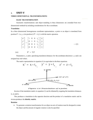
1. 4. UNIT-V
THREE DIMENSIONAL TRANSFORMATIONS
BASIC TRANSFORMATION
Geometric transformations and object modeling in three dimensions are extended from two-
dimensional methods by including considerations for the z-coordinate.
Translation
This produces a translation in the opposite direction and the product of a translation matrix and its
inverse produces the identity matrix.
Rotation
 To generate a rotation transformation for an object an axis of rotation must be designed to rotate
the object and the amount of angular rotation is also be specified.
In a three dimensional homogeneous coordinate representation, a point or an object is translated from
position P = (x, y, z) to position () P' = x',y',z with the matrix operation.
Parameters tx, ty and tz specifying translation distances for the coordinate directions x, y and z are
assigned any real values.
The matrix representation in equation (1) in equivalent to the three equations.
Inverse of the translation matrix in equation (1) can be obtained by negating the translation distances
tx, ty and tz.

2.  Positive rotation angles produce counter clockwise rotations about a coordinate axis.
Co-ordinate Axes Rotations
The 2D z axis rotation equations are easily extended to 3D.
Substituting permutations (5) in Equation (2), we get the equations for an x-axis rotation:
Parameters θ specifies the rotation angle. In homogeneous coordinate form, the 3D z axis rotation
equations are expressed as
Transformation equations for rotation about the other two coordinate axes can be obtained
with a
cyclic permutation of the coordinate parameters x, y and z in equation (2) i.e., we use the replacements.

3. which can be written in the homogeneous coordinate form
Rotation of an object around the x-axis is demonstrated in Figure 4.8.
Cyclically permuting coordinates in equation (6) give the transformation equation for a y axis
rotation.
The matrix representation for y-axis rotation is
An example of y axis rotation is shown in Figure 4.9.

4.  An inverse rotation matrix is formed by replacing the rotation angle θ by –θ.
 Negative values for rotation angles generate rotations in a clockwise direction, so the identity
matrix is produced when any rotation matrix is multiplied by its inverse.
 Since only the sine function is affected by the change in sign of the rotation angle, the inverse
matrix can also be obtained by interchanging rows and columns. (i.e.) we can calculate the
inverse of any rotation matrix R by evaluating its transpose (R–1 = RT).
General Three Dimensional Rotations
 A rotation matrix for any axis that does not coincide with a coordinate axis can be set up as a
composite transformation involving combinations of translations and the coordinate axes
rotations.
 We obtain the required composite matrix by
(1) Setting up the transformation sequence that moves the selected rotation axis onto one of the
coordinate axes.
(2) Then set up the rotation matrix about that coordinate axis for the specified rotation angle.
(3) Obtaining the inverse transformation sequence that returns the rotation axis to its original
position.
 In the special case where an object is to be rotated about an axis that is parallel to one of the
coordinate axes, we can attain the desired rotation with the following transformation sequence
(1) Translate the object so that the rotation axis coincides with the parallel coordinate axis.
(2) Perform the specified rotation about that axis.
(3) Translate the object so that the rotation axis is moved back to its original position.
 When an object is to be rotated about an axis that is not parallel to one of the coordinate axes, we
need to perform some additional transformations.
 In such case, we need rotations to align the axis with a selected coordinate axis and to bring the
axis back to its original orientation.

5.  Given the specifications for the rotation axis and the rotation angle, we can accomplish the
required rotation in five steps: 
(1) Translate the object so that the rotation axis passes through the coordinate origin.
(2) Rotate the object so that the axis of rotation coincides with one of the coordinate axes.
(3) Perform the specified rotation about that coordinate axis.
(4) Apply inverse rotations to bring the rotation axis back to its original orientation.
(5) Apply the inverse translation to bring the rotation axis back to its original position.
Scaling
The matrix expression for the scaling transformation of a position P = (x, y, z) relative to the
coordinate origin can be written as
 Where scaling parameters sx, sy and sz are assigned any position values.
 Explicit expressions for the coordinate transformations for scaling relative to the origin are
 Scaling an object changes the size of the object and repositions the object relative to the
coordinate origin.
 If the transformation parameters are not equal, relative dimensions in the object are changed.
 The origin shape of the object is preserved with a uniform scaling (sx = sy = sz). (Figure 4.10)
shows the result of scaling an object uniformly with each scaling parameter set to 2.

6.  Scaling with respect to a selected fixed position (xf, yf, zf) can be represented with the following
transformation sequence:
(1) Translate the fixed point to the origin.
(2) Scale the object relative to the coordinate origin using equation (11).
(3) Translate the fixed point back to its original position.
This sequence of transformation is shown in Figure 4.11.
The matrix representation for an arbitrary fixed point scaling can be expressed as the
concatenation of the translate-scale-translate transformations are

7.  Inverse scaling matrix m formed by replacing the scaling parameters sx, sy and sz with their
reciprocals.
 The inverse matrix generates an opposite scaling transformation, so the concatenation of any
scaling matrix and its inverse produces the identity matrix.
OTHER TRANSFORMATIONS
Reflections
 Reflections about other planes can be obtained as a combination of rotations and coordinate plane
reflections.
Shears
 Shearing transformations are used to modify object shapes.
 They are also used in three dimensional viewing for obtaining general projections
transformations.
 The following transformation produces a z-axis shear.
 Parameters a and b can be assigned any real values.
 This transformation matrix is used to alter x and y coordinate values by an amount that is
proportional to the z value, and the z coordinate will be changed.
 Boundaries of planes that are perpendicular to the z axis are shifted by an amount proportional to
 A 3D reflection can be performed relative to a selected reflection axis or with respect to a
selected reflection plane.
 Reflection relative to a given axis are equivalent to 180° rotations about the axis.
 When the reflection plane in a coordinate plane (either xy, xz or yz) then the transformation can
a conversion between left-handed and right-handed systems.
 An example of a reflection that converts coordinate specifications from a right handed system to a
left-handed system is shown in Figure 4.12.
 This transformation changes the sign of z coordinates, leaves the x and y coordinate values
unchanged.
 The matrix representation for this reflection of points relative to the xy plane is

8. z figure 4.13 shows the effect of shearing matrix on a unit cube for the values a = b = 1.
CLASSIFICATION OF VISIBLE SURFACE DETECTION ALGORTHIM
Visible face detection algorithms are broadly classified according to
whether they deal with object definitions directly or with their projected
images. These two approaches are called object-space methods and image
space methods.
An object-space method compares objects and parts of objects to each
other within the scene definition to determine which surfaces, as a whole,
we should label as visible. In a image-space algorithm, visibility is decided
point by point at each pixel position on the projection plane. Most visible-
surface algorithms use image-space methods, although object-space
methods can be used effectively locate visible surfaces in some cases. Line-
display algorithms, on the other hand, generally use object-space methods
to identify visible lines in wire-frame displays, but many image-space
visible-surface algorithms can be adapted easily to visible-line detection.
BACK-FACE DETECTION
 A fast and simple object-space method for identifying the back faces of a polyhedron is based on
the „inside-outside‟ tests.
 A point (x, y, z) is “inside” a polygon surface with plane parameters A, B, C and D if
Ax + By+ Cz + D < 0
 When an inside point is along the line of sight to the surface, the polygon must be a backface.
 This test is done by considering the normal N to a polygon surface, which has Casterian
components (A, B, C).

9.  If V is a vector in the viewing direction from the eye (or “camera”) position, then the polygon is a
backface if
V.N > 0
 If object descriptions have been connected to projection coordinates and the viewing direction is
parallel to the viewing Zv axis then V = (0, 0, Vz) and
V . N = Vz . C
 So we have to consider the sign of C, the z component of the normal vector N. It is shown in
Figure.5.14.
 In a right-handed viewing system with viewing direction along the negative Zv axis (Figure.5.15)
the polygon is back-face if C < 0.
 If C = 0, we cannot see any face, since the viewing direction is graying that polygon.
 Thus we can label any polygon as a back-face if its normal vector has a Z component value
C ≤ 0
 Back-faces have normal vectors that point away from the viewing position and are identified by C
³ 0 when the viewing direction is along the positive Zv axis.

10. DEPTH BUFFER METHOD (OR) Z- BUFFER ALGORITHM
 This method compares surface depths at each pixel position on the projection plane.
 The surface depth is measured from the view plane along the Z axis of a viewing system.
 When object description is converted to projection coordinates (x, y, z), each pixel position on the
view plane is specified by x and y coordinate, and z value gives the depth information. Thus
object depths can be compared by comparing the z-values.
 The Z buffer algorithm is usually implemented in the normalized coordinates, so that z values
range from 0 at the back clipping plane to 1 at the front clipping plane.
 The implementation requires another buffer memory called z-buffer along with the frame buffer
memory required for raster display devices.
 A z-buffer is used to store depth values for each (x, y) position as surfaces are processed and the
frame buffer stores the intensity values for each position.
 At the beginning, z-buffer is initialized to 0, representing the z-value at the back clipping plane
and the frame buffer is initialized to the background color.
 Each surface listed in the display file is then processed one scan line at a time, calculating the
depth (z value) at each (x, y) pixel position.
 The calculated depth value is compared to the value previously stored in the z-buffer at that
position.
 If the calculated depth value is greater than the value stored in the z-buffer, the new depth value is
stored, and the surface intensity at that position is determined and placed in the same x,y location
in the frame buffer.
 For example in the following Fig.5.16 among three surfaces, surface s has the smallest depth at
view position (x, y) and hence highest z value. So it is visible at that position.

11. Z-buffer Algorithm
Step-1: Initialize the z-buffer and frame buffer so that for all buffer positions
Z-buffer (x, y) = 0 and frame buffer(x, y) = Ibackground
Step-2: During scan conversion process, for each position on each polygon surface, compare
depth values to previously stored values in the depth buffer to determine visibility.
Calculate z-value for each (x,y) position on the polygon.
Advantages
(1) It is very easy to implement.
(2) It can be implemented in hardware to overcome the speed problem.
(3) Since the algorithm processes objects one at a time, the total number of polygons in a
picture can be arbitrarily large.
If z>Z-buffer(x,y) then set
Step-3: Stop
 After processing all the surfaces, the z-buffer, contains depth values for the variable surfaces and
the frame buffer contains the corresponding intensity values for those surfaces.
 To calculate z-values, the plane equation
Ax + By + Cz + D =0
 is used where (x, y, z) is any point on the plane, and the coefficient A, B, C and D are constants
describing the spatial properties of the plane.
 If at (x,y), the above equation evaluates to z, then at (x+Dx, y) the value of z is
 Only one subtraction is needed to calculate z(x+1, y), given z(x, y) since the quotient A/C is
constant and Δx=1.
 A similar incremental calculation can be performed to determine the first value of z on the next
scanline, decrementing by B/C for each Δy.

12. Disadvantages
(1) It requires an additional buffer and hence the large memory.
(2) It is a time consuming process as it requires comparison for each pixel instead of the
entire polygon.
BUFFER METHOD
 An extension of the ideas in the depth buffer method is the A-buffer method.
 A-buffer method represents an antialiased, area-averaged, accumulation-buffer method.
 It expands the depth buffer so that each position in the buffer can reference a linked list of
surfaces.
 More than one surface intensity can be taken into consideration at each pixel position and object
edges can be antialiased.
 Each position in the A-buffer has 2 fields.
(1) Depth field-stores a positive or negative real number.
(2) Intensity field-stores surface-intensity information or a pointer value.
 If the depth field is positive, the number stored at that position in the depth of a single surface
overlapping the corresponding pixel area.
 The intensity field stores the RGB components of the surface color at that point and the percent of
pixel coverage.
 If the depth field is negative, it indicates multiple surface contributions to the pixel intensity.
 The intensity field stores a pointer to a linked list of surface data.
 The data for each surface in the linked list includes :
1. RGB intensity components.
2. Opacity parameter.
3. Depth.
4. Percent of area coverage.
5. Surface identifier.
6. Other surface rendering parameters.
7. Pointer to next surface.
 The A-buffer can be constructed using methods similar to those in the depth-buffer algorithm.
 Scan lines are processed to determine surface overlaps of pixels across the individual scan lines.
 Surfaces are subdivided into a polygon mesh and clipped against the pixel boundaries.
 Using the opacity factors and percent of surface overlaps, the intensity of each pixel is calculated
as an average of the contributions from the overlapping surfaces.

13. SCANLINE METHOD
 A Scan line method of hidden surface removal is an another approach of image space method.
 This method deals with more than one surface.
 As each scanline is processed, it examines all polygon surfaces intersecting that line to determine
which are visible.
 It performs the depth calculation and finds which polygon is nearest to the view plane.
 For the positions along this scan line between edges AD and BC, only the flag for surface S1 is
ON.
 Therefore, no depth calculations are necessary and intensity information for flag for surface S2 is
ON and during that position of scan line the intensity information for surface S2 is entered into
 Finally, it enters the intensity value of the nearest polygon at that position into the frame buffer.
 The scanline algorithm maintains active edge list.
 The active edge list contains only edges that cross the current scan line, sorted in order
ofincreasing x. scanline method of hidden surface removal also stores a flag for each surface
that is set ONor OFF to indicate whether a position along a scan line is inside or outside of the
surface.
 Scanlines are processed from left to right.ftmost boundary of the surface, the surface flag is
turned ON, and at the rightmostboundary, it is turned OFF.
The Figure.5.17 illustrates the scanline method for hidden surface removal. Here, the active edge list
for scanline 1 contains the information for edges AD, BC, EH, and FG.

14.  the frame buffer.
 For scan line 2, the active edge list contains edges AD, EH, BC and FG.
Along the scan line 2from edge AD to edge EH, only the flag for surface S1
is ON.
 Between edges EH and BC, the flags for both surfaces are ON. In this
portion of scanline2, thedepth calculations are necessary.
Here we have assumed that the depth of S1 is less than the depth of S2 and hence the intensitiesof
surface S1