70th SWCS International Annual Conference July 26-29, 2015 Greensboro, NC

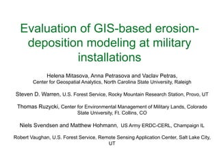
1. Evaluation of GIS-based erosion-
deposition modeling at military
installations
Helena Mitasova, Anna Petrasova and Vaclav Petras,
Center for Geospatial Analytics, North Carolina State University, Raleigh
Steven D. Warren, U.S. Forest Service, Rocky Mountain Research Station, Provo, UT
Thomas Ruzycki, Center for Environmental Management of Military Lands, Colorado
State University, Ft. Collins, CO
Niels Svendsen and Matthew Hohmann, US Army ERDC-CERL, Champaign IL
Robert Vaughan, U.S. Forest Service, Remote Sensing Application Center, Salt Lake City,
UT

2. Soil erosion on installations
Soil erosion on military training facilities is due to disturbances by tracked
and wheeled vehicles, exploding munitions, and construction
Damage is expensive to repair and diminishes the realism of the training
experience, and jeopardizes the safety of soldiers and equipment.
Sediment transport from installations also creates off-site impacts -
sediment is the single largest contributor to non-point source pollution.
Limited field data combined with imagery and RUSLE model estimates
indicated reduction of soil erosion since 50ies thanks to
conservation programs

3. Soil disturbances from training
Tracked and wheeled vehicles compact the soil and damage vegetation

4. Gully erosion
Soil erosion may accelerate as the soil surface becomes increasingly disturbed
and protective vegetation is lost as a result of the cumulative impacts of military
training. Extensive damage from gullying may occur

5. Erosion modeling for installations
Erosion modeling has been used to support land management,
conservation and sediment control
Spatially aggregated USLE or RUSLE, only potential sediment sources
mapped no deposition considered
Very limited experimental spatially distributed data available
Simplicity important at installation scale
GIS-based models developed in 90s to support land management
systems: mapping erosion and deposition, process-based simulations

6. GIS based erosion models
Landscape scale mapping of potential sediment sources (and sinks)
Identification of locations vulnerable to soil erosion and deposition in areas
with complex topography and variable land cover
USLE3D or RUSLE3D
E = R.K.C.P.L.S
LS = Am.(sin β)n
Where E is soil loss, R is rainfall, K is soil, C is cover and LS is topographic factor, A
is normalized upslope are per unit width and β is normalized slope angle
Simplified Erosion-Deposition (SED) model
T = R.K.C.P.Um.(sin η)n
ED = ∇ · (T s0) = ∂(T cos α)/∂x + ∂(T sin α)/∂y
Where T is sediment transport capacity, ED is erosion/deposition, U is contributing
area per unit width, η is slope, α is aspect (flow direction)

7. GIS based models
Complex topography,
uniform land cover and
soils:
USLE3D:
Detachment capacity
limited erosion, no
deposition
SED model
Transport capacity limited
erosion and deposition
Represent two extreme cases –
actual erosion/deposition
dynamically transitions between
these two

8. GIS-based models: variable cover
Variable land cover: C-factor map
USLE3D: variable soil loss rate
SED: variable soil loss rate and
deposition along the land cover
change edge
erosion deposition

9. SED model for installation
Ft. Hood, TX area
used in on-line tutorial
http://ncsu-osgeorel.github.io/erosion-modeling-tutorial/index.html
http://ncsu-osgeorel.github.io/erosion-modeling-tutorial/index.htm

10. Input data
10m resolution DEM K-factor from SSURGO
converted to 10m resolution raster

11. Land cover C-factor
Landsat8 bands with field data correlation (r2 ~ 0.4 – 0.8)
NLCD with values assigned using USDA tables
Landsat and NAIP with high resolution estimates at points sampled
at unsupervised classes
NDVI derived from Landsat C-factor derived from correlation
between NDVI and field observations

12. Topographic factor for complex terrain
Topographic factor is based on parameters derived from DEM
Different flow routing techniques: MFD for dispersal flow, least cost path for routing
through depressions without filling them
Exponents m,n control influence of flow accumulation versus slope
Slope Flow accumulation Topographic factor
LS=Um.(sin η)n

13. Erosion and deposition map
Sediment flow ~ sediment transport capacity Change in sediment flow: erosion and
deposition
T = R.K.C.P.Um.(sin η)n ED = ∇ · (T s0) = ∂(T cos α)/∂x + ∂(T sin α)/∂y

14. Erosion / deposition evaluation
Modeled erosion/deposition classes were compared with visual field
estimates at random points generated in each class
Results were mixed: Issues with C-factor estimates, model resolution
versus local features, quality of DEM, selection of validation points

15. Yakima, WA
C-factor based on Landsat: installation wide and zoomed-in
Points show transects where C-factor was estimated in the field
C-factor map was computed from correlation between the field-based C-factor
and Landsat8 bands

16. Yakima
Transport capacity map – installation-wide and zoom in

17. Yakima
Modeled erosion/deposition:
installation-wide and zoom-in with observed points
51 points with observed erosion/deposition
~ 64% classified within 1 class
Often neighboring cells have correct class

18. Yakima
Very complex, dynamic erosion/deposition pattern
DEM from USGS NED has potential artifacts (pits).
10-30m resolution overestimates extent of concentrated flow areas

19. Current research
SUAS and lidar mapping – adaptive, precision conservation based on repeated,
high resolution mapping
Process-based simulations used to explore, prioritize and optimize conservation
measures

20. Tangible Landscape
Exploring surface runoff and erosion and sediment control design using
tangible physical model with near real-time feedback
Ft. Bragg
application

21. Conclusions
Erosion/deposition patterns at military installations are complex and require
higher resolution than 10m to avoid overestimation of concentrated flows
Reliable and efficient C-factor estimation remains major challenge and
would require extensive field work
Mapping by sUAS/lidar can provide erosion/deposition data needed to
calibrate/validate erosion models at landscape scale – we anticipate
possible innovations in theory if the current models cannot consistently
reproduce the observed patterns and rates
Tutorial for GRASS and ArcGIS available in github, improvements and
contributions are welcome
http://ncsu-osgeorel.github.io/erosion-modeling-tutorial/