SlideShare a Scribd company logo
1 of 81
UNIT III: NON LINEAR DATA STRUCTURES – TREES 9
Tree ADT –Unbalanced tree –Balanced tree- tree traversals - Binary Tree ADT – expression trees
– applications of trees – binary search tree ADT –Threaded Binary Trees- AVL Trees – B-Tree -
B+ Tree - Heap –Binary Heap- Applications of heap.
TREES
Tree is a Non- Linear data structure in which data are stored in a hierarchal manner. It is
also defined as a collection of nodes. The collection can be empty. Otherwise, a tree consists
of a distinguished node r, called the root, and zero or more (sub) trees T1, T2, . . . , Tk, each
of whose roots are connected by a directed edge to r.
The root of each subtree is said to be a child of r, and r is the parent of each subtree
root. A tree is a collection of n nodes, one of which is the root, and n - 1 edges. That there
are n - 1 edges follows from the fact that each edge connects some node to its parent and
every node except the root has one parent
Generic tree
A tree
Terms in Tree
In the tree above figure, the root is A.
✔ Node F has A as a parent and K, L, and M as children.
✔ Each node may have an arbitrary number of children, possibly zero.
✔ Nodes with no children are known as leaves;
✔ The leaves in the tree above are B, C, H, I, P, Q, K, L, M, and N.
✔ Nodes with the same parent are siblings; thus K, L, and M are all siblings.
Grandparent and grandchild relations can be defined in a similar manner.
✔ A path from node n1 to nk is defined as a sequence of nodes n1, n2, . . . , nk such that ni
is the parent of ni+1 for 1 i < k.
✔ The length of this path is the number of edges on the path, namely k -1.
✔ There is a path of length zero from every node to itself.
✔ For any node ni, the depth of ni is the length of the unique path from the root
to ni. Thus, the root is at depth 0.
✔ The height of ni is the longest path from ni to a leaf. Thus all leaves are at height 0.
✔ The height of a tree is equal to the height of the root.
Example: For the above tree,
E is at depth 1 and height 2;
F is at depth 1 and height 1; the height of the tree is 3. T
Note:
✔ The depth of a tree is equal to the depth of the deepest leaf; this is always
equal to the height of the tree.
✔ If there is a path from n1 to n2, then n1 is an ancestor of n2 and n2 is a
descendant of n1. If n1 n2, then n1 is a proper ancestor of n2 and n2 is a
proper descendant of n1.
✔ A tree there is exactly one path from the root to each node.
Types of the Tree
Based on the no. of children for each node in the tree, it is classified into two to types.
1. Binary tree
2. General tree
Binary tree
In a tree, each and every node has a maximum of two children. It can be empty,
one or two. Then it is called as Binary tree.
Eg:
General Tree
In a tree, node can have any no of children. Then it is called as general Tree.
Eg:
Implementation of Trees
Tree can be implemented by two methods.
1. Array Implementation
2. Linked List implementation
Apart from these two methods, it can also be represented by First Child and Next
sibling Representation.
One way to implement a tree would be to have in each node, besides its data, a pointer to
each child of the node. However, since the number of children per node can vary so greatly and
is not known in advance, it might be infeasible to make the children direct links in the data
structure, because there would be too much wasted space. The solution is simple: Keep the
children of each node in a linked list of tree nodes.
Node declarations for trees
typedef struct tree_node *tree_ptr;
struct tree_node
{
element_type element;
tree_ptr first_child;
tree_ptr next_sibling;
};
First child/next sibling representation of the tree shown in the below Figure
Arrows that point downward are first_child pointers. Arrows that go left to right are
next_sibling pointers. Null pointers are not drawn, because there are too many. In the above tree,
node E has both a pointer to a sibling (F) and a pointer to a child (I), while some nodes have
neither.
Tree Traversals
Visiting of each and every node in a tree exactly only once is called as Tree traversals.
Here Left subtree and right subtree are traversed recursively.
Types of Tree Traversal:
1. Inorder Traversal
2. Preorder Traversal
3. Postorder Traversal
Inorder traversal:
Rules:
● Traverse Left subtree recursively
● Process the node
● Traverse Right subtree recursively
Eg
Inorder traversal: a + b*c + d*e + f*g.
Preorder traversal:
Rules:
● Process the node
● Traverse Left subtree recursively
● Traverse Right subtree recursively
Preorder traversal: ++a*b c*+*d e f g
Postorder traversal:
Rules:
● Traverse Left subtree recursively
● Traverse Right subtree recursively
● Process the node
Postorder traversal: a b c*+de*f + g* +
Tree Traversals with an Application
There are many applications for trees. Most important two applications are,
1. Listing a directory in a hierarchical file system
2. Calculating the size of a directory
1. Listing a directory in a hierarchical file system
One of the popular uses is the directory structure in many common operating systems,
including UNIX, VAX/VMS, and DOS.
Typical directories in the UNIX file system (UNIX directory)
✔ The root of this directory is /usr. (The asterisk next to the name indicates that /usr is itself
a directory.)
✔ /usr has three children, mark, alex, and bill, which are themselves directories. Thus, /usr
contains three directories and no regular files.
✔ The filename /usr/mark/book/ch1.r is obtained by following the leftmost child three times.
Each / after the first indicates an edge; the result is the full pathname.
✔ Two files in different directories can share the same name, because they must have
different paths from the root and thus have different pathnames.
✔ A directory in the UNIX file system is just a file with a list of all its children, so the
directories are structured almost exactly in accordance with the type declaration.
✔ Each directory in the UNIX file system also has one entry that points to itself and another
entry that point to the parent of the directory. Thus, technically, the UNIX file system is
not a tree, but is treelike.
Routine to list a directory in a hierarchical file system void
list_directory ( Directory_or_file D )
{
list_dir ( D, 0 ); }
Void list_dir ( Directory_or_file D, unsigned int depth )
{
if ( D is a legitimate entry)
{
print_name ( depth, D );
if( D is a directory )
for each child, c, of D
list_dir( c, depth+1 );
} }
The logic of the algorithm is as follow.
✔ The argument to list_dir is some sort of pointer into the tree. As long as the pointer is
valid, the name implied by the pointer is printed out with the appropriate number of tabs.
✔ If the entry is a directory, then we process all children recursively, one by one. These
children are one level deeper, and thus need to be indenting an extra space.
This traversal strategy is known as a preorder traversal. In a preorder traversal, work at a
node is performed before (pre) its children are processed. If there are n file names to be output,
then the running time is O (n).
2. Calculating the size of a directory
As above UNIX Directory Structure, the numbers in parentheses representing the number
of disk blocks taken up by each file, since the directories are themselves files, they have sizes
too. Suppose we would like to calculate the total number of blocks used by all the files in the tree.
Here the work at a node is performed after its children are evaluated. So it follows Postorder
traversal.
The most natural way to do this would be to find the number of blocks contained in the
subdirectories /usr/mark (30), /usr/alex (9), and /usr/bill (32). The total number of blocks is then
the total in the subdirectories (71) plus the one block used by /usr, for a total of 72.
Routine to calculate the size of a directory unsigned
int size_directory( Directory_or_file D )
{
unsigned int total_size;
total_size = 0;
if( D is a legitimate entry)
{
total_size = file_size( D );
if( D is a directory )
for each child, c, of D
total_size += size_directory( c );
}
return( total_size );
}
Binary Trees
A binary tree is a tree in which no node can have more than two children.
Figure shows that a binary tree consists of a root and two subtrees, Tl and
Tr, both of which could possibly be empty.
Worst-case binary tree
Implementation
A binary tree has at most two children; we can keep direct pointers to them. The
declaration of tree nodes is similar in structure to that for doubly linked lists, in that a node is a
structure consisting of the key information plus two pointers (left and right) to other nodes.
Binary tree node declarations
typedef struct tree_node *tree_ptr;
struct tree_node
{
element_type element;
tree_ptr left;
tree_ptr right;
};
typedef tree_ptr TREE;
Expression Trees
When an expression is represented in a binary tree, then it is called as an expression Tree. The
leaves of an expression tree are operands, such as constants or variable names, and the other nodes
contain operators. It is possible for nodes to have more than two children. It is also possible for a
node to have only one child, as is the case with the unary minus operator.
We can evaluate an expression tree, T, by applying the operator at the root to the values
obtained by recursively evaluating the left and right subtrees.
In our example, the left subtree evaluates to a + (b * c) and the right subtree evaluates to
((d *e) + f ) *g. The entire tree therefore represents (a + (b*c)) + (((d * e) + f)* g).
We can produce an (overly parenthesized) infix expression by recursively producing a
parenthesized left expression, then printing out the operator at the root, and finally recursively
producing a parenthesized right expression. This general strattegy ( left, node, right ) is known
as an inorder traversal; it gives Infix Expression.
An alternate traversal strategy is to recursively print out the left subtree, the
right subtree, and then the operator. If we apply this strategy to our tree above, the output is a b c
* + d e * f + g * +, which is called as postfix Expression. This traversal strategy is generally
known as a postorder traversal.
A third traversal strategy is to print out the operator first and then recursively print out the
left and right subtrees. The resulting expression, + + a * b c * + * d e f g, is the less useful prefix
notation and the traversal strategy is a preorder traversal
Expression tree for (a + b * c) + ((d * e + f ) * g)
Constructing an Expression Tree
Algorithm to convert a postfix expression into an expression tree
1. Read the postfix expression one symbol at a time.
2. If the symbol is an operand, then
a. We create a one node tree and push a pointer to it onto a stack.
3. If the symbol is an operator,
a. We pop pointers to two trees T1 and T2 from the stack (T1 is popped first) and
form a new tree whose root is the operator and whose left and right children point
to T2 and T1 respectively.
4. A pointer to this new tree is then pushed onto the stack.
Suppose the input is
a b + c d e + * *
The first two symbols are operands, so we create one-node trees and push pointers to
them onto a stack.
Next, a '+' is read, so two pointers to trees are popped, a new tree is formed, and a pointer to it is
pushed onto the stack.
Next, c, d, and e are read, and for each a one-node tree is created and a pointer
to the corresponding tree is pushed onto the stack.
Now a '+' is read, so two trees are merged. Continuing, a '*' is read, so we pop two tree pointers
and form a new tree with a '*' as root.
Finally, the last symbol is read, two trees are merged, and a pointer to the final
tree is left on the stack.
The Search Tree ADT-Binary Search Tree
The property that makes a binary tree into a binary search tree is that for every
node, X, in the tree, the values of all the keys in the left subtree are smaller than the key
value in X, and the values of all the keys in the right subtree are larger than the key value
in X.
Notice that this implies that all the elements in the tree can be ordered in some consistent
manner.
In the above figure, the tree on the left is a binary search tree, but the tree on the right is
not. The tree on the right has a node with key 7 in the left subtree of a node with key 6. The
average depth of a binary search tree is O(log n).
Binary search tree declarations
typedef struct tree_node *tree_ptr;
struct tree_node
{
element_type element;
tree_ptr left;
tree_ptr right;
};
typedef tree_ptr SEARCH_TREE;
Make Empty:
This operation is mainly for initialization. Some programmers prefer to initialize the first
element as a one-node tree, but our implementation follows the recursive definition of trees more
closely.
Find
This operation generally requires returning a pointer to the node in tree T that has key x,
or NULL if there is no such node. The structure of the tree makes this simple. If T is , then we
can just return . Otherwise, if the key stored at T is x, we can return T. Otherwise, we make a
recursive call on a subtree of T, either left or right, depending on the relationship of x to the key
stored in T.
Routine to make an empty tree
SearchTree makeempty (search tree T)
{
if(T!=NULL)
{
Makeempty (T->left);
Makeempty (T->Right);
Free( T);
}
return NULL; }
Routine for Find operation
Position find( Elementtype X, SearchTree T )
{
if( T == NULL )
return NULL;
if( x < T->element )
return( find( x, T->left ) );
else
if( x > T->element )
return( find( x, T->right ) );
else
return T;
}
FindMin & FindMax:
These routines return the position of the smallest and largest elements in the
tree, respectively.
To perform a findmin, start at the root and go left as long as there is a left child. The
stopping point is the smallest element.
The findmax routine is the same, except that branching is to the right child.
Recursive implementation of Findmin for binary search trees
Position findmin( SearchTree T )
{
if( T == NULL )
return NULL;
else
if( T->left == NULL )
return( T );
else
return( findmin ( T->left ) );
}
Recursive implementation of FindMax for binary search trees
Position findmax( SearchTree T )
{
if( T == NULL )
return NULL;
else
if( T->Right == NULL )
return( T );
else
return( findmax( T->right ) );
}
Nonrecursive implementation of FindMin for binary search trees
Position findmin( SearchTree T )
{
if( T != NULL )
while( T->left != NULL )
T=T->left;
return(T);
}
Nonrecursive implementation of FindMax for binary search trees
Position findmax( SearchTree T )
{
if( T != NULL )
while( T->right != NULL )
T=T->right;
return(T);
}
Insert
To insert x into tree T, proceed down the tree. If x is found, do nothing. Otherwise,
insert x at the last spot on the path traversed.
To insert 5, we traverse the tree as though a find were occurring. At the node with key 4,
we need to go right, but there is no subtree, so 5 is not in the tree, and this is the correct spot.
Insertion routine
Since T points to the root of the tree, and the root changes on the first insertion, insert is
written as a function that returns a pointer to the root of the new tree.
searchTree insert( elementtype x, SearchTree T )
{
if( T == NULL )
{
T = (SEARCH_TREE) malloc ( sizeof (struct tree_node) );
if( T == NULL )
fatal_error("Out of space!!!");
else
{
T->element = x;
T->left = T->right = NULL; }
}
else
if( x < T->element )
T->left = insert( x, T->left );
else
if( x > T->element )
T->right = insert( x, T->right );
/* else x is in the tree already. We'll do nothing */
return T; }
Delete
Once we have found the node to be deleted, we need to consider several possibilities.
If the node is a leaf, it can be deleted immediately.
If the node has one child, the node can be deleted after its parent adjusts a pointer to
bypass the node
if a node with two children. The general strategy is to replace the key of this node with
the smallest key of the right subtree and recursively delete that node. Because the smallest node
in the right subtree cannot have a left child, the second
delete is an easy one.
The node to be deleted is the left child of the root; the key value is 2. It is replaced with
the smallest key in its right subtree (3), and then that node is deleted as before.
Deletion of a node (4) with one child, before and after
Deletion of a node (2) with two children, before and after
If the number of deletions is expected to be small, then a popular strategy to
use is lazy deletion: When an element is to be deleted, it is left in the tree and merely marked as
being deleted.
Deletion routine for binary search trees
Searchtree delete( elementtype x, searchtree T )
{
Position tmpcell;
if( T == NULL )
error("Element not found");
else
if( x < T->element ) /* Go left */
T->left = delete( x, T->left );
else
if( x > T->element ) /* Go right */
T->right = delete( x, T->right );
else /* Found element to be deleted */
if( T->left && T->right ) /* Two children */
{
tmp_cell = find_min( T->right );
T->element = tmp_cell->element;
T->right = delete( T->element, T->right );
}
else /* One child */
{
tmpcell = T;
if( T->left == NULL ) /* Only a right child */
T= T->right;
if( T->right == NULL ) /* Only a left
child */ T = T->left;
free( tmpcell );
}
return T;
}
Average-Case Analysis of BST
✔ All of the operations of the previous section, except makeempty, should take O(log
n) time, because in constant time we descend a level in the tree, thus operating on a
tree that is now roughly half as large.
✔ The running time of all the operations, except makeempty is O(d), where d is the
depth of the node containing the accessed key.
✔ The average depth over all nodes in a tree is O(log n).
✔ The sum of the depths of all nodes in a tree is known as the internal path length.
Threaded Binary Tree
● A binary tree is threaded by making all right child pointers that would normally be null
point to the inorder successor of the node (if it exists), and all left child pointers that
would normally be null point to the inorder predecessor of the node.
● We have the pointers reference the next node in an inorder traversal; called threads
● We need to know if a pointer is an actual link or a thread, so we keep a boolean for each
pointer
Why do we need Threaded Binary Tree?
● Binary trees have a lot of wasted space: the leaf nodes each have 2 null pointers. We can
use these pointers to help us in inorder traversals.
● Threaded binary tree makes the tree traversal faster since we do not need stack or
recursion for traversal
Types of threaded binary trees:
● Single Threaded: each node is threaded towards either the in-order
predecessor or successor (left orright) means all right null pointers will point to inorder
successor OR all left null pointers will point to inorder predecessor.
● Double threaded: each node is threaded towards both the in-order
predecessor and successor (left andright) means all right null pointers will point to
inorder successor AND all left null pointers will point to inorder predecessor.
Single Threaded: each node is threaded towards either the in-order predecessor or successor
(left or right) means all right null pointers will point to inorder successor OR all left null
pointers will point to inorder predecessor.
Implementation:
Let’s see how the Node structure will look like
class Node{
Node left;
Node right;
int data;
boolean rightThread;
public Node(int data){
this.data = data;
rightThread = false;
}
}
In normal BST node we have left and right references and data but in threaded binary tree
we have boolean another field called “rightThreaded”. This field will tell whether node’s
right pointer is pointing to its inorder successor, but how, we will see it further.
Operations:
We will discuss two primary operations in single threaded binary tree
1. Insert node into tree
2. Print or traverse the tree.( here we will see the advantage of threaded tree)
Insert():
The insert operation will be quite similar to Insert operation in Binary search tree with few
modifications.
● To insert a node our first task is to find the place to insert the node.
● Take current = root .
● start from the current and compare root.data with n.
● Always keep track of parent node while moving left or right.
● if current.data is greater than n that means we go to the left of the root, if after moving to left,
the current = null then we have found the place where we will insert the new node. Add the
new node to the left of parent node and make the right pointer points to parent node and
rightThread = true for new node.
●
● if current.data is smaller than n that means we need to go to the right of the root, while going
into the right subtree, check rightThread for current node, means right thread is provided and
points to the in order successor, if rightThread = false then and current reaches to null, just
insert the new node else if rightThread = true then we need to detach the right pointer (store
the reference, new node right reference will be point to it) of current node and make it point to
the new node and make the right reference point to stored reference. (See image and code for
better understanding)
Traverse():
traversing the threaded binary tree will be quite easy, no need of any recursion or any stack
for storing the node. Just go to the left most node and start traversing the tree using right
pointer and whenever rightThread = false again go to the left most node in right subtree.
(See image and code for better understanding)
Double threaded:
Each node is threaded towards both the in-order predecessor and successor (left and right)
means all right null pointers will point to inorder successor AND all left null pointers will
point to inorder predecessor.
Implementation:
Let’s see how the Node structure will look like
class Node {
int data;
int leftBit;
int rightBit;
Node left;
Node right;
public Node(int data) {
this.data = data;
}
}
If you notice we have two extra fields in the node than regular binary tree node. leftBit and
rightBit. Let’s see what these fields represent.
leftBit=0 left reference points to the inorder predecessor
leftBit=1 left reference points to the left child
rightBit=0 right reference points to the inorder successor
righBit=1 right reference points to the right child
Let’s see why do we need these fields and why do we need a dummy node when If we try to
convert the normal binary tree to threaded binary
Now if you see the picture above , there are two references left most reference and right
most reference pointers has nowhere to point to.
Need of a Dummy Node: As we saw that references left most reference and right most
reference pointers has nowhere to point to so we need a dummy node and this node will
always present even when tree is empty.
In this dummy node we will put rightBit = 1 and its right child will point to it self and leftBit
= 0, so we will construct the threaded tree as the left child of dummy node.
Let’s see how the dummy node will look like:
Now we will see how this dummy node will solve our problem of references left most
reference and right most reference pointers has nowhere to point to.
Double Threaded binary tree with dummy node
Now we will see the some operations in double threaded binary tree.
Insert():
The insert operation will be quite similar to Insert operation in Binary search tree with few
modifications.
1. To insert a node our first task is to find the place to insert the node.
2. First check if tree is empty, means tree has just dummy node then then insert the new node into
left subtree of the dummy node.
3. If tree is not empty then find the place to insert the node, just like in normal BST.
4. If new node is smaller than or equal to current node then check if leftBit =0, if yes then we
have found the place to insert the node, it will be in the left of the subtree and if leftBit=1 then
go left.
5. If new node is greater than current node then check if rightBit =0, if yes then we have found
the place to insert the node, it will be in the right of the subtree and if rightBit=1 then go right.
6. Repeat step 4 and 5 till the place to be inserted is not found.
7. Once decided where the node will be inserted, next task would be to insert the node. first we
will see how the node will be inserted as left child.
n.left = current.left;
current.left = n;
n.leftBit = current.leftBit;
current.leftBit = 1;
n.right = current;
see the image below for better understanding
8. To insert the node as right child.
n.right = current.right;
current.right = n;
n.rightBit = current.rightBit;
current.rightBit = 1;
n.left = current;
see the image below for better understanding.
Traverse():
Now we will see how to traverse in the double threaded binary tree, we do not need a
recursion to do that which means it won’t require stack, it will be done n one single traversal
in O(n).
Starting from left most node in the tree, keep traversing the inorder successor and print
it.(click here to read more about inorder successor in a tree).
See the image below for more understanding.
AVL Trees
The balance condition and allow the tree to be arbitrarily deep, but after every
operation, a restructuring rule is applied that tends to make future operations efficient. These
types of data structures are generally classified as self-adjusting.
An AVL tree is identical to a binary search tree, except that for every node in the
tree, the height of the left and right subtrees can differ by at most 1. (The height of an empty
tree is defined to be -1.)
An AVL (Adelson-Velskii and Landis) tree is a binary search tree with a balance
condition. The simplest idea is to require that the left and right subtrees have the same height.
The balance condition must be easy to maintain, and it ensures that the depth of the tree is
O(log n).
The above figure shows, a bad binary tree. Requiring balance at the root is not enough.
In Figure, the tree on the left is an AVL tree, but the tree on the right is not.
Thus, all the tree operations can be performed in O(log n) time, except possibly insertion.
When we do an insertion, we need to update all the balancing information for the nodes
on the path back to the root, but the reason that insertion is difficult is that inserting a node could
violate the AVL tree property.
Inserting a node into the AVL tree would destroy the balance condition.
Let us call the unbalanced node α. Violation due to insertion might occur in four cases:
1. An insertion into the left subtree of the left child of α
2. An insertion into the right subtree of the left child of α
3. An insertion into the left subtree of the right child of α
4. An insertion into the right subtree of the right child of α
Violation of AVL property due to insertion can be avoided by doing some modification
on the node α. This modification process is called as Rotation.
Types of rotation
1. Single Rotation
2. Double Rotation
Single Rotation (case 1) – Single rotate with Left
The two trees in the above Figure contain the same elements and are both binary search
trees.
First of all, in both trees k1 < k2. Second, all elements in the subtree X are smaller than
k1 in both trees. Third, all elements in subtree Z are larger than k2. Finally, all elements in subtree
Y are in between k1 and k2. The conversion of one of the above trees to the other is known as a
rotation.
In an AVL tree, if an insertion causes some node in an AVL tree to lose the balance
property: Do a rotation at that node.
The basic algorithm is to start at the node inserted and travel up the tree, updating the balance
information at every node on the path.
In the above figure, after the insertion of the in the original AVL tree on the left, node 8 becomes
unbalanced. Thus, we do a single rotation between 7 and 8, obtaining the tree on the right.
Routine :
Static position Singlerotatewithleft( Position K2)
{
Position k1;
K1=k2->left;
K2->left=k1->right;
K1->right=k2;
K2->height=max(height(k2->left),height(k2->right));
K1->height=max(height(k1->left),k2->height);
Return k1;
}
Single Rotation (case 4) – Single rotate with Right
(Refer diagram from Class note)
Suppose we start with an initially empty AVL tree and insert the keys 1 through 7 in
sequential order. The first problem occurs when it is time to insert key 3, because the AVL
property is violated at the root. We perform a single rotation between the root and its right child
to fix the problem. The tree is shown in the following figure, before and after the rotation.
A dashed line indicates the two nodes that are the subject of the rotation. Next, we insert the key
4, which causes no problems, but the insertion of 5 creates a violation at node 3, which is fixed
by a single rotation.
Next, we insert 6. This causes a balance problem for the root, since its left subtree is of
height 0, and its right subtree would be height 2. Therefore, we perform a single rotation at the
root between 2 and 4.
The rotation is performed by making 2 a child of 4 and making 4's original left subtree
the new right subtree of 2. Every key in this subtree must lie between 2 and 4, so this
transformation makes sense. The next key we insert is 7, which causes another rotation.
Routine :
Static position Singlerotatewithright( Position K1)
{
Position k2;
K2=k1->right;
K1->right=k2->left;
K2->left=k1;
K1->height=max(height(k1->left),height(k1->right));
K2->height=max(height(k2->left),k1->height);
Return k2;
}
Double Rotation
(Right-left) double rotation
(Left-right) double rotation
In the above diagram, suppose we insert keys 8 through 15 in reverse order. Inserting 15 is easy,
since it does not destroy the balance property, but inserting 14 causes a height imbalance at node
7.
As the diagram shows, the single rotation has not fixed the height imbalance. The problem is that
the height imbalance was caused by a node inserted into the tree containing the middle elements
(tree Y in Fig. (Right-left) double rotation) at the same time as the other trees had identical
heights. This process is called as double rotation, which is similar to a single rotation but
involves four subtrees instead of three.
In our example, the double rotation is a right-left double rotation and involves 7, 15, and
14. Here, k3 is the node with key 7, k1 is the node with key 15, and
k2 is the node with key 14.
Next we insert 13, which require a double rotation. Here the double rotation is again a
right-left double rotation that will involve 6, 14, and 7 and will restore the tree. In this case, k3 is
the node with key 6, k1 is the node with key 14, and k2 is the node with key 7. Subtree A is the
tree rooted at the node with key 5, subtree B is the empty subtree that was originally the left child
of the node with key 7, subtree C is the tree rooted at the node with key 13, and finally, subtree
D is the tree rooted at the node with key 15.
If 12 is now inserted, there is an imbalance at the root. Since 12 is not between
4 and 7, we know that the single rotation will work. Insertion of 11 will require a single rotation:
To insert 10, a single rotation needs to be performed, and the same is true for the
subsequent insertion of 9. We insert 8 without a rotation, creating the almost perfectly balanced
tree.
Routine for double Rotation with left (Case 2)
Static position doublerotatewithleft(position k3)
{
K3->left=singlerotatewithright(k3->left);
Return singlerotatewithleft(k3);
}
Routine for double Rotation with right (Case 3)
Static position doublerotatewithlright(position k1)
{
K1->right=singlerotatewithleft(k1->right);
Return singlerotatewithright(k1);
}
Node declaration for AVL trees:
typedef struct avlnode *position;
typedef struct avlnode *avltree;
struct avlnode
{
elementtype element;
avltree left;
avltree right;
int height;
};
typedef avl_ptr SEARCH_TREE;
Routine for finding height of an AVL node
Int height (avltree p)
{
if( p == NULL )
return -1;
else
return p->height;
}
Routine for insertion of new element into a AVL TREE
(Refer Class note)
B-Trees
AVL tree and Splay tree are binary; there is a popular search tree that is not binary. This
tree is known as a B-tree.
A B-tree of order m is a tree with the following structural properties:
a. The root is either a leaf or has between 2 and m children.
b. All nonleaf nodes (except the root) have between m/2 and m children.
c. All leaves are at the same depth.
All data is stored at the leaves. Contained in each interior node are pointers
p1, p2, . . . , pm to the children, and values k1, k2, . . . , km - 1, representing the smallest key
found in the subtrees p2, p3, . . . , pm respectively. Some of these pointers might be NULL, and
the corresponding ki would then be undefined.
For every node, all the keys in subtree p1 are smaller than the keys in subtree p2, and so on. The
leaves contain all the actual data, which is either the keys themselves or pointers to records
containing the keys.
The number of keys in a leaf is also between m/2 and m.
An example of a B-tree of order 4
A B-tree of order 4 is more popularly known as a 2-3-4 tree, and a B-tree of order 3 is
known as a 2-3 tree
Our starting point is the 2-3 tree that follows.
We have drawn interior nodes (nonleaves) in ellipses, which contain the two pieces of
data for each node. A dash line as a second piece of information in an interior node indicates that
the node has only two children. Leaves are drawn in boxes, which contain the keys. The keys in
the leaves are ordered.
To perform a find, we start at the root and branch in one of (at most) three directions,
depending on the relation of the key we are looking for to the two values stored at the node.
When we get to a leaf node, we have found the correct place to put x. Thus, to insert a
node with key 18, we can just add it to a leaf without causing any violations of the 2-3 tree
properties. The result is shown in the following figure.
If we now try to insert 1 into the tree, we find that the node where it belongs is already
full. Placing our new key into this node would give it a fourth element which is not allowed. This
can be solved by making two nodes of two keys each and adjusting the information in the parent.
To insert 19 into the current tree, two nodes of two keys each, we obtain the following tree.
This tree has an internal node with four children, but we only allow three per node.
Again split this node into two nodes with two children. Now this node might be one of three
children itself, and thus splitting it would create a problem for its parent but we can keep on
splitting nodes on the way up to the root until we either get to the root or find a node with only
two children.
If we now insert an element with key 28, we create a leaf with four children, which is
split into two leaves of two children.
This creates an internal node with four children, which is then split into two children. Like
to insert 70 into the tree above, we could move 58 to the leaf containing 41 and 52, place 70 with
59 and 61, and adjust the entries in the internal nodes.
Deletion in B-Tree
● If this key was one of only two keys in a node, then its removal leaves only one key. We can
fix this by combining this node with a sibling. If the sibling has three keys, we can steal one
and have both nodes with two keys.
● If the sibling has only two keys, we combine the two nodes into a single node with three
keys. The parent of this node now loses a child, so we might have to percolate this strategy
all the way to the top.
● If the root loses its second child, then the root is also deleted and the tree becomes one level
shallower.
We repeat this until we find a parent with less than m children. If we split the root, we create
a new root with two children.
The depth of a B-tree is at most log m/2 n.
The worst-case running time for each of the insert and delete operations is thus O(m logm
n) = O( (m / log m ) log n), but a find takes only O(log n ).
B+ Tree
● B+ Tree is an extension of B Tree which allows efficient insertion, deletion and search operations.
● In B Tree, Keys and records both can be stored in the internal as well as leaf nodes. Whereas, in B+ tree,
records (data) can only be stored on the leaf nodes while internal nodes can only store the key values.
● The leaf nodes of a B+ tree are linked together in the form of a singly linked lists to make the search
queries more efficient.
● B+ Tree are used to store the large amount of data which can not be stored in the main memory. Due to
the fact that, size of main memory is always limited, the internal nodes (keys to access records) of the B+
tree are stored in the main memory whereas, leaf nodes are stored in the secondary memory.
● The internal nodes of B+ tree are often called index nodes. A B+ tree of order 3 is shown in the
following figure.
B+ Tree
Advantages of B+ Tree
● Records can be fetched in equal number of disk accesses.
● Height of the tree remains balanced and less as compare to B tree.
● We can access the data stored in a B+ tree sequentially as well as directly.
● Keys are used for indexing.
● Faster search queries as the data is stored only on the leaf nodes.
B Tree VS B+ Tree
S.NO B Tree B+ Tree
1 Search keys can not be repeatedly stored. Redundant search keys can be present.
2 Data can be stored in leaf nodes as well as
internal nodes
Data can only be stored on the leaf nodes.
3 Searching for some data is a slower process
since data can be found on internal nodes as
well as on the leaf nodes.
Searching is comparatively faster as data can
only be found on the leaf nodes.
4 Deletion of internal nodes are so
complicated and time consuming.
Deletion will never be a complexed process since
element will always be deleted from the leaf
nodes.
5 Leaf nodes can not be linked together. Leaf nodes are linked together to make the search
operations more efficient.
Insertion in B+ Tree
Step 1: Insert the new node as a leaf node
Step 2: If the leaf doesn't have required space, split the node and copy the middle node to the
next index node.
Step 3: If the index node doesn't have required space, split the node and copy the middle element
to the next index page.
Example :
Insert the value 195 into the B+ tree of order 5 shown in the following figure.
195 will be inserted in the right sub-tree of 120 after 190. Insert it at the desired position.
The node contains greater than the maximum number of elements i.e. 4, therefore split it and
place the median node up to the parent.
Now, the index node contains 6 children and 5 keys which violates the B+ tree properties,
therefore we need to split it, shown as follows.
Deletion in B+ Tree
Step 1: Delete the key and data from the leaves.
Step 2: if the leaf node contains less than minimum number of elements, merge down the node
with its sibling and delete the key in between them.
Step 3: if the index node contains less than minimum number of elements, merge the node with
the sibling and move down the key in between them.
Example
Delete the key 200 from the B+ Tree shown in the following figure.
200 is present in the right sub-tree of 190, after 195. delete it.
Merge the two nodes by using 195, 190, 154 and 129.
Now, element 120 is the single element present in the node which is violating the B+ Tree
properties. Therefore, we need to merge it by using 60, 78, 108 and 120.
Now, the height of B+ tree will be decreased by 1.
PRIORITY QUEUES (HEAPS)
A queue is said to be priority queue, in which the elements are dequeued based on the
priority of the elements.
A priority queue is used in,
● Jobs sent to a line printer are generally placed on a queue. For instance, one job might be
particularly important, so that it might be desirable to allow that job to be run as soon as the
printer is available.
● In a multiuser environment, the operating system scheduler must decide which of several
processes to run. Generally a process is only allowed to run for a fixed period of time. One
algorithm uses a queue. Jobs are initially placed at the end of the queue. The scheduler will
repeatedly take the first job on the queue, run it until either it finishes or its time limit is up,
and place it at the end of the queue. This strategy is generally not appropriate, because very
short jobs will seem to take a long time because of the wait involved to run. Generally, it is
important that short jobs finish as fast as possible. This is called as Shortest Job First (SJF).
This particular application seems to require a special kind of queue, known as a priority
queue.
Basic model of a priority queue
A priority queue is a data structure that allows at least the following two operations:
1. Insert, equivalent of enqueue
2. Deletemin, removes the minimum element in the heap equivalent of the
Queue’s dequeue operation.
Implementations of Priority Queue
1. Array Implementation
2. Linked list Implementation
3. Binary Search Tree implementation
4. Binary Heap Implementation
Array Implementation
Drawbacks:
1. There will be more wastage of memory due to maximum size of the array should be define
in advance
2. Insertion taken at the end of the array which takes O (N) time.
3. Delete_min will also take O (N) times.
Linked list Implementation
It overcomes first two problems in array implementation. But delete_min operation
takes O(N) time similar to array implementation.
Binary Search Tree implementation
Another way of implementing priority queues would be to use a binary search tree. This
gives an O(log n) average running time for both operations.
Binary Heap Implementation
Another way of implementing priority queues would be to use a binary heap. This gives
an O(1) average running time for both operations.
Binary Heap
Like binary search trees, heaps have two properties, namely, a structure property and a heap
order property. As with AVL trees, an operation on a heap can destroy one of the properties, so
a heap operation must not terminate until all heap properties are in order.
1. Structure Property
2. Heap Order Property
Structure Property
A heap is a binary tree that is completely filled, with the possible exception of the
bottom level, which is filled from left to right. Such a tree is known as a complete binary
tree.
A complete Binary Tree
A complete binary tree of height h has between 2h and 2h+1 - 1 nodes. This implies that
the height of a complete binary tree is log n, which is clearly O(log n).
Array implementation of complete
binary tree Note:
For any element in array position i, the left child is in position 2i, the right
child is in the cell after the left child (2i + 1), and the parent is in position
i/2 .
The only problem with this implementation is that an estimate of the maximum heap
size is required in advance.
Types of Binary
Heap Min Heap
A binary heap is said to be Min heap such that any node x in the heap, the key value of
X is smaller than all of its descendants children.
Max Heap
A binary heap is said to be Min heap such that any node x in the heap, the key
value of X is larger than all of its descendants children.
It is easy to find the minimum quickly, it makes sense that the smallest element should be
at the root. If we consider that any subtree should also be a heap, then any node should be smaller
than all of its descendants.
Applying this logic, we arrive at the heap order property. In a heap, for every node X, the
key in the parent of X is smaller than (or equal to) the key in X.
Similarly we can declare a (max) heap, which enables us to efficiently find and remove
the maximum element, by changing the heap order property. Thus, a priority queue can be used
to find either a minimum or a maximum.
By the heap order property, the minimum element can always be found at the root.
Declaration for priority queue
struct heapstruct
{
int capacity;
int size;
element_type *elements;
};
typedef struct heapstruct *priorityQ;
Create routine of priority Queue
priorityQ create (int max_elements )
{
priorityQ H;
if( max_elements < MIN_PQ_SIZE )
error("Priority queue size is too small");
H = (priorityQ) malloc ( sizeof (struct heapstruct) );
if( H == NULL )
fatal_error("Out of space!!!");
H->elements = (element_type *) malloc( ( max_elements+1) * sizeof (element_type) );
if( H->elements == NULL )
fatal_error("Out of space!!!");
H->capacity= max_elements;
H->size = 0;
H->elements[0] = MIN_DATA;
return H; }
Basic Heap Operations
It is easy to perform the two required operations. All the work involves ensuring that the
heap order property is maintained.
1. Insert
2. Deletemi
n Insert
To insert an element x into the heap, we create a hole in the next available location, since
otherwise the tree will not be complete.
If x can be placed in the hole without violating heap order, then we do so and are done.
Otherwise we slide the element that is in the hole's parent node into the hole, thus bubbling the
hole up toward the root. We continue this process until x can be placed in the hole.
Figure shows that to insert 14, we create a hole in the next available heap location.
Inserting 14 in the hole would violate the heap order property, so 31 is slide down into the hole.
This strategy is continued until the correct location for 14 is found. This general strategy
is known as a percolate up; the new element is percolated up the heap until the correct location
is found.
We could have implemented the percolation in the insert routine by performing repeated
swaps until the correct order was established, but a swap requires three assignment statements. If
an element is percolated up d levels, the number of assignments performed by the swaps would
be 3d. Our method uses d + 1 assignments.
Routine to insert into a binary heap
/* H->element[0] is a sentinel */
Void insert( element_type x, priorityQ H )
{
int i;
if( is_full( H ) )
error("Priority queue is full");
else
{
i = ++H->size;
while( H->elements[i/2] > x )
{
H->elements[i] = H->elements[i/2];
i /= 2;
} H->elements[i] = x; } }
If the element to be inserted is the new minimum, it will be pushed all the way to the top.
The time to do the insertion could be as much as O (log n), if the element to be inserted is the
new minimum and is percolated all the way to the root. On
Deletemin
Deletemin are handled in a similar manner as insertions. Finding the minimum is easy;
the hard part is removing it.
When the minimum is removed, a hole is created at the root. Since the heap now becomes
one smaller, it follows that the last element x in the heap must move somewhere in the heap. If x
can be placed in the hole, then we are done. This is unlikely, so we slide the smaller of the hole's
children into the hole, thus pushing the hole down one level. We repeat this step until x can be
placed in the hole. This general strategy is known as a percolate down.
In Figure, after 13 is removed, we must now try to place 31 in the heap. 31 cannot be
placed in the hole, because this would violate heap order. Thus, we place the smaller child (14)
in the hole, sliding the hole down one level. We repeat this again, placing 19 into the hole and
creating a new hole one level deeper. We then place 26 in the hole and create a new hole on the
bottom level. Finally, we are able to place 31 in the hole.
Routine to perform deletemin in a binary heap
element_type delete_min( priorityQ H )
{
int i, child;
element_type min_element, last_element;
if( is_empty( H ) )
{
error("Priority queue is empty");
return H->elements[0];
}
min_element = H->elements[1];
last_element = H->elements[H->size--];
for( i=1; i*2 <= H->size; i=child )
{
child = i*2;
if( ( child != H->size ) && ( H->elements[child+1] < H->elements [child] ) )
child++;
if( last_element > H->elements[child] )
H->elements[i] = H->elements[child];
else
break;
}
H->elements[i] = last_element;
return min_element;
}
The worst-case running time for this operation is O(log n). On average, the element that
is placed at the root is percolated almost to the bottom of the heap, so the average running time
is O (log n).
Other Heap Operations
The other heap operations are
1. Decreasekey
2. Increasekey
3. Delete
4. Buildheap
Decreasekey
The decreasekey(x, ∆, H) operation lowers the value of the key at position x by a positive
amount ∆. Since this might violate the heap order, it must be fixed by a percolate up.
USE:
This operation could be useful to system administrators: they can make their programs
run with highest priority.
Increasekey
The increasekey(x, ∆, H) operation increases the value of the key at position x by a
positive amount ∆. This is done with a percolate down.
USE:
Many schedulers automatically drop the priority of a process that is consuming
excessive CPU time.
Delete
The delete(x, H) operation removes the node at position x from the heap. This is done by
first performing decreasekey(x,∆ , H) and then performing deletemin(H). When a process is
terminated by a user, it must be removed from the priority queue.
Buildheap
The buildheap(H) operation takes as input n keys and places them into an empty heap.
This can be done with n successive inserts. Since each insert will take O(1) average and O(log
n) worst-case time, the total running time of this algorithm would be O(n) average but O(n log
n) worst-case.
UNIT IV : NON LINEAR DATA STRUCTURES – GRAPHS 9
Definition – Representation of Graph – Types of graph - Breadth-first traversal - Depth-first
traversal – Topological Sort – Bi-connectivity – Cut vertex – Euler circuits – Applications of
graphs-minimum spanning tree-dijkstra's algorithm-kruskal's algorithm
Graph
A graph can be defined as group of vertices and edges that are used to connect these vertices. A graph can
be seen as a cyclic tree, where the vertices (Nodes) maintain any complex relationship among them instead
of having parent child relationship.
Definition
A graph G can be defined as an ordered set G(V, E) where V(G) represents the set of vertices and E(G)
represents the set of edges which are used to connect these vertices.
A Graph G(V, E) with 5 vertices (A, B, C, D, E) and six edges ((A,B), (B,C), (C,E), (E,D), (D,B), (D,A)) is
shown in the following figure.
Directed and Undirected Graph
A graph can be directed or undirected. However, in an undirected graph, edges are not associated with the
directions with them. An undirected graph is shown in the above figure since its edges are not attached with
any of the directions. If an edge exists between vertex A and B then the vertices can be traversed from B to
A as well as A to B.
In a directed graph, edges form an ordered pair. Edges represent a specific path from some vertex A to
another vertex B. Node A is called initial node while node B is called terminal node.
A directed graph is shown in the following figure.
Graph Terminology
Path
A path can be defined as the sequence of nodes that are followed in order to reach some terminal node V
from the initial node U.
Closed Path
A path will be called as closed path if the initial node is same as terminal node. A path will be closed path
if V0=VN.
Simple Path
If all the nodes of the graph are distinct with an exception V0=VN, then such path P is called as closed simple
path.
Cycle
A cycle can be defined as the path which has no repeated edges or vertices except the first and last vertices.
Connected Graph
A connected graph is the one in which some path exists between every two vertices (u, v) in V. There are
no isolated nodes in connected graph.
Complete Graph
A complete graph is the one in which every node is connected with all other nodes. A complete graph
contain n(n-1)/2 edges where n is the number of nodes in the graph.
Weighted Graph
In a weighted graph, each edge is assigned with some data such as length or weight. The weight of an edge
e can be given as w(e) which must be a positive (+) value indicating the cost of traversing the edge.
Digraph
A digraph is a directed graph in which each edge of the graph is associated with some direction and the
traversing can be done only in the specified direction.
Loop
An edge that is associated with the similar end points can be called as Loop.
Adjacent Nodes
If two nodes u and v are connected via an edge e, then the nodes u and v are called as neighbours or adjacent
nodes.
Degree of the Node
A degree of a node is the number of edges that are connected with that node. A node with degree 0 is called
as isolated node.
Graph representation
In this article, we will discuss the ways to represent the graph. By Graph representation, we simply mean
the technique to be used to store some graph into the computer's memory.
A graph is a data structure that consist a sets of vertices (called nodes) and edges. There are two ways to
store Graphs into the computer's memory:
o Sequential representation (or, Adjacency matrix representation)
o Linked list representation (or, Adjacency list representation)
In sequential representation, an adjacency matrix is used to store the graph. Whereas in linked list
representation, there is a use of an adjacency list to store the graph.
Representation of Graphs
1. Adjacency matrix / Incidence Matrix
2. Adjacency Linked List/ Incidence Linked List
Adjacency matrix
We will consider directed graphs. (Fig. 1)
Now we can number the vertices, starting at 1. The graph shown in above figure represents 7
vertices and 12 edges.
One simple way to represent a graph is to use a two-dimensional array. This is known as
an adjacency matrix representation.
For each edge (u, v), we set a[u][v]= 1; otherwise the entry in the array is 0. If the edge has a
weight associated with it, then we can set a[u][v] equal to the weight and use either a very large
or a very small weight as a sentinel to indicate nonexistent edges.
Advantage is, it is extremely simple, and the space requirement is (|V|2
).
For directed graph
A[u][v]= { 1, if there is edge from u to v
0 otherwise }
For undirected graph
A[u][v]= { 1, if there is edge between u and v
0 otherwise }
For weighted graph
A[u][v]= { value , if there is edge from u to v
∞, if no edge between u and v }
Adjacency lists
Adjacency lists are the standard way to represent graphs. Undirected graphs can be
similarly represented; each edge (u, v) appears in two lists, so the space usage essentially doubles.
A common requirement in graph algorithms is to find all vertices adjacent to some given vertex
v, and this can be done, in time proportional to the number of such vertices found, by a simple
scan down the appropriate adjacency list.
An adjacency list representation of a graph (See above fig 5.1)
Topological Sort
A topological sort is an ordering of vertices in a directed acyclic graph, such that if there
is a path from vi to vj, then vj appears after vi in the ordering.
It is clear that a topological ordering is not possible if the graph has a cycle, since for
two vertices v and w on the cycle, v precedes w and w precedes v.
Directed acyclic graph
In the above graph v1, v2, v5, v4, v3, v7, v6 and v1, v2, v5, v4, v7, v3, v6 are both
topological orderings.
A simple algorithm to find a topological ordering
First, find any vertex with no incoming edges (Source vertex). We can then print this
vertex, and remove it, along with its edges, from the graph.
To formalize this, we define the indegree of a vertex v as the number of edges (u,v). We
compute the indegrees of all vertices in the graph. Assuming that the indegree array is initialized
and that the graph is read into an adjacency list,
Indegree Before Dequeue #
Vertex 1 2 3 4 5 6 7
v1 0 0 0 0 0 0 0
v2 1 0 0 0 0 0 0
v3 2 1 1 1 0 0 0
v4 3 2 1 0 0 0 0
v5 1 1 0 0 0 0 0
v6 3 3 3 3 2 1 0
v7 2 2 2 1 0 0 0
Enqueue v1 v2 v5 v4 v3 v7 v6
Dequeue v1 v2 v5 v4 v3 v7 v6
Simple Topological Ordering Routine
Void topsort( graph G )
{
unsigned int counter;
vertex v, w;
for( counter = 0; counter < NUM_VERTEX; counter++ )
{
v = find_new_vertex_of_indegree_zero( );
if( v = NOT_A_VERTEX )
{
error("Graph has a cycle");
break;
}
top_num[v] = counter;
for each w adjacent to v
indegree[w]--;
}
}
Explanation
The function find_new_vertex_of_indegree_zero scans the indegree array looking for a
vertex with indegree 0 that has not already been assigned a topological number. It returns
NOT_A_VERTEX if no such vertex exists; this indicates that the graph has a cycle.
Routine to perform Topological Sort
Void topsort( graph G )
{
QUEUE Q;
unsigned int counter;
vertex v, w;
Q = create_queue( NUM_VERTEX );
makeempty( Q );
counter = 0;
for each vertex v
if( indegree[v] = 0 )
enqueue( v, Q );
while( !isempty( Q ) )
{
v = dequeue( Q );
top_num[v] = ++counter; /* assign next number */
for each w adjacent to v
if( --indegree[w] = 0 )
enqueue( w, Q );
}
if( counter != NUMVERTEX )
error("Graph has a cycle");
dispose_queue( Q ); /* free the memory */
}
Graph Traversal:
Visiting of each and every vertex in the graph only once is called as Graph traversal.
There are two types of Graph traversal.
1. Depth First Traversal/ Search (DFS)
2. Breadth First Traversal/ Search (BFS)
Depth First Traversal/ Search (DFS)
Depth-first search is a generalization of preorder traversal. Starting at some vertex, v, we
process v and then recursively traverse all vertices adjacent to v. If this process is performed on
a tree, then all tree vertices are systematically visited in a total of O(|E|) time, since |E| = (|V|).
We need to be careful to avoid cycles. To do this, when we visit a vertex v, we mark it
visited, since now we have been there, and recursively call depth-first search on all adjacent
vertices that are not already marked.
The two important key points of depth first search
1. If path exists from one node to another node walk across the edge – exploring
the edge
2. If path does not exist from one specific node to any other nodes, return to the
previous node where we have been before – backtracking
Procedure for DFS
Starting at some vertex V, we process V and then recursively traverse all the vertices adjacent to
V. This process continues until all the vertices are processed. If some vertex is not processed
recursively, then it will be processed by using backtracking. If vertex W is visited from V, then
the vertices are connected by means of tree edges. If the edges not included in tree, then they are
represented by back edges. At the end of this process, it will construct a tree called as DFS tree.
Routine to perform a depth-first search void
void dfs( vertex v )
{
visited[v] = TRUE;
for each w adjacent to v
if( !visited[w] )
dfs( w );
}
The (global) boolean array visited[ ] is initialized to FALSE. By recursively calling the
procedures only on nodes that have not been visited, we guarantee that we do not loop
indefinitely.
* An efficient way of implementing this is to begin the depth-first search at v1. If we need to
restart the depth-first search, we examine the sequence vk, vk + 1, . . . for an unmarked
vertex,where vk - 1 is the vertex where the last depth-first search was started.
An undirected graph
Steps to construct depth-first spanning tree
a. We start at vertex A. Then we mark A as visited and call dfs(B) recursively. dfs(B) marks
B as visited and calls dfs(C) recursively.
b. dfs(C) marks C as visited and calls dfs(D) recursively.
c. dfs(D) sees both A and B, but both these are marked, so no recursive calls are made.
dfs(D) also sees that C is adjacent but marked, so no recursive call is made there, and
dfs(D) returns back to dfs(C).
d. dfs(C) sees B adjacent, ignores it, finds a previously unseen vertex E adjacent, and thus
calls dfs(E).
e. dfs(E) marks E, ignores A and C, and returns to dfs(C).
f. dfs(C) returns to dfs(B). dfs(B) ignores both A and D and returns.
g. dfs(A) ignores both D and E and returns.
Depth-first search of the graph
---------> Back edge
Tree edge
The root of the tree is A, the first vertex visited. Each edge (v, w) in the graph is present in
the tree. If, when we process (v, w), we find that w is unmarked, or if, when we process (w, v),
we find that v is unmarked, we indicate this with a tree edge.
If when we process (v, w), we find that w is already marked, and when processing (w, v), we find
that v is already marked, we draw a dashed line, which we will call a back edge, to indicate that
this "edge" is not really part of the tree.
Breadth First Traversal (BFS)
Here starting from some vertex v, and its adjacency vertices are processed. After all the adjacency
vertices are processed, then selecting any one the adjacency vertex and process will continue. If
the vertex is not visited, then backtracking is applied to visit the unvisited vertex.
Routine:
void BFS (vertex v)
{
visited[v]= true;
For each w adjacent to v
If (!visited[w])
visited[w] = true;
}
Example of BFS algorithm
Now, let's understand the working of BFS algorithm by using an example. In the example given below,
there is a directed graph having 7 vertices.
In the above graph, minimum path 'P' can be found by using the BFS that will start from Node A
and end at Node E. The algorithm uses two queues, namely QUEUE1 and QUEUE2. QUEUE1 holds
all the nodes that are to be processed, while QUEUE2 holds all the nodes that are processed and
deleted from QUEUE1.
Now, let's start examining the graph starting from Node A.
Step 1 - First, add A to queue1 and NULL to queue2.
1. QUEUE1 = {A}
2. QUEUE2 = {NULL}
Step 2 - Now, delete node A from queue1 and add it into queue2. Insert all neighbors of node A to
queue1.
1. QUEUE1 = {B, D}
2. QUEUE2 = {A}
Step 3 - Now, delete node B from queue1 and add it into queue2. Insert all neighbors of node B to
queue1.
1. QUEUE1 = {D, C, F}
2. QUEUE2 = {A, B}
Step 4 - Now, delete node D from queue1 and add it into queue2. Insert all neighbors of node D to
queue1. The only neighbor of Node D is F since it is already inserted, so it will not be inserted again.
1. QUEUE1 = {C, F}
2. QUEUE2 = {A, B, D}
Step 5 - Delete node C from queue1 and add it into queue2. Insert all neighbors of node C to queue1.
1. QUEUE1 = {F, E, G}
2. QUEUE2 = {A, B, D, C}
Step 5 - Delete node F from queue1 and add it into queue2. Insert all neighbors of node F to queue1.
Since all the neighbors of node F are already present, we will not insert them again.
1. QUEUE1 = {E, G}
2. QUEUE2 = {A, B, D, C, F}
Step 6 - Delete node E from queue1. Since all of its neighbors have already been added, so we will
not insert them again. Now, all the nodes are visited, and the target node E is encountered into queue2.
1. QUEUE1 = {G}
2. QUEUE2 = {A, B, D, C, F, E}
Difference between DFS & BFS
S. No DFS BFS
1 Back tracking is possible from a dead end. Back tracking is not possible.
2 Vertices from which exploration is
incomplete are processed in a LIFO order.
The vertices to be explored are
organized as a FIFO queue.
3 Search is done in one particular direction at
the time.
The vertices in the same level are
maintained parallel. (Left to right) (
alphabetical ordering)
Bi-connectivity / Bi connected Graph:
An undirected graph is called Biconnected if there are two vertex-disjoint paths between any two
vertices. In a Biconnected Graph, there is a simple cycle through any two vertices.
By convention, two nodes connected by an edge form a biconnected graph, but this does not
verify the above properties. For a graph with more than two vertices, the above properties must
be there for it to be Biconnected.
Or in other words:
A graph is said to be Biconnected if:
1. It is connected, i.e. it is possible to reach every vertex from every other vertex, by a simple path.
2. Even after removing any vertex the graph remains connected.
Following are some examples:
How to find if a given graph is Biconnected or not?
A connected graph is Biconnected if it is connected and doesn’t have any Articulation Point. We
mainly need to check two things in a graph.
1. The graph is connected.
2. There is not articulation point in graph.
We start from any vertex and do DFS traversal. In DFS traversal, we check if there is any
articulation point. If we don’t find any articulation point, then the graph is Biconnected. Finally,
we need to check whether all vertices were reachable in DFS or not. If all vertices were not
reachable, then the graph is not even connected.
Articulation points
If a graph is not biconnected, the vertices whose removal would disconnect the graph
are known as articulation points.
The above graph is not biconnected: C and D are articulation points.
The removal of C would disconnect G, and the removal of D would disconnect E and F, from
the rest of the graph.
Depth-first search provides a linear-time algorithm to find all articulation points in a
connected graph.
● First, starting at any vertex, we perform a depth-first search and number the nodes
as they are visited.
● For each vertex v, we call this preorder number num (v). Then, for every vertex v
in the depth-first search spanning tree, we compute the lowest-numbered vertex,
which we call low(v), that is reachable from v by taking zero or more tree edges
and then possibly one back edge (in that order).
By the definition of low, low (v) is the minimum of
1. num(v)
2. the lowest num(w) among all back edges (v, w)
3. the lowest low(w) among all tree edges (v, w)
The first condition is the option of taking no edges, the second way is to choose no tree
edges and a back edge, and the third way is to choose some tree edges and possibly a back edge.
The depth-first search tree in the above Figure shows the preorder number first, and then the
lowest-numbered vertex reachable under the rule described above.
The lowest-numbered vertex reachable by A, B, and C is vertex 1 (A), because they can all take
tree edges to D and then one back edge back to A and find low value for all other vertices.
Depth-first tree that results if depth-first search starts at C
To find articulation points,
● The root is an articulation point if and only if it has more than one child, because if it has
two children, removing the root disconnects nodes in different subtrees, and if it has only
one child, removing the root merely disconnects the root.
● Any other vertex v is an articulation point if and only if v has some child w such that low
(w)>= num (v). Notice that this condition is always satisfied at the root;
We examine the articulation points that the algorithm determines, namely C and D. D has a child
E, and low (E)>= num (D), since both are 4. Thus, there is only one way for E to get to any node
above D, and that is by going through D.
Similarly, C is an articulation point, because low (G)>= num (C).
Routine to assign num to vertices
Void assignnum( vertex v )
{
vertex w;
num[v] = counter++;
visited[v] = TRUE;
for each w adjacent to v
if( !visited[w] )
{
parent[w] = v;
assignnum ( w ); } }
Routine to compute low and to test for articulation
Void assignlow( vertex v )
{
vertex w;
low[v] = num[v]; /* Rule 1 */
for each w adjacent to v
{
if( num[w] > num[v] ) /* forward edge */
{
assignlow( w );
if( low[w] >= num[v] )
printf( "%v is an articulation pointn", v );
low[v] = min( low[v], low[w] ); /* Rule 3 */
}
else
if( parent[v] != w ) /* back edge */
low[v] = min( low[v], num[w] ); /* Rule 2 */ } }
Testing for articulation points in one depth-first search (test for the root is omitted) void
findart( vertex v )
{
vertex w;
visited[v] = TRUE;
low[v] = num[v] = counter++; /* Rule 1 */
for each w adjacent to v
{
if( !visited[w] ) /* forward edge */
{
parent[w] = v;
findart( w );
if( low[w] >= num[v] )
printf ( "%v is an articulation pointn", v );
low[v] = min( low[v], low[w] ); /* Rule */
}
else
if( parent[v] != w ) /* back edge */
low[v] = min( low[v], num[w] ); /* Rule 2 */
}
}
Euler Circuits
We must find a path in the graph that visits every edge exactly once. If we are to solve the
"extra challenge," then we must find a cycle that visits every edge exactly once. This graph
problem was solved in 1736 by Euler and marked the beginning of graph theory. The problem is
thus commonly referred to as an Euler path or Euler tour or Euler circuit problem, depending
on the specific problem statement.
Consider the three figures as shown below. A popular puzzle is to reconstruct these figures
using a pen, drawing each line exactly once. The pen may not be lifted from the paper while the
drawing is being performed. As an extra challenge, make the pen finish at the same point at which
it started.
Three drawings
1. The first figure can be drawn only if the starting point is the lower left- or right-hand
corner, and it is not possible to finish at the starting point.
2. The second figure is easily drawn with the finishing point the same as the starting point.
3. The third figure cannot be drawn at all within the parameters of the puzzle.
We can convert this problem to a graph theory problem by assigning a vertex to each
intersection. Then the edges can be assigned in the natural manner, as in figure.
The first observation that can be made is that an Euler circuit, which must end on its starting
vertex, is possible only if the graph is connected and each vertex has an even degree (number of
edges). This is because, on the Euler circuit, a vertex is entered and then left.
If exactly two vertices have odd degree, an Euler tour, which must visit every edge but need not
return to its starting vertex, is still possible if we start at one of the odd-degree vertices and finish
at the other.
If more than two vertices have odd degree, then an Euler tour is not possible.
That is, any connected graph, all of whose vertices have even degree, must have an
Euler circuit
As an example, consider the graph in
The main problem is that we might visit a portion of the graph and return to the starting point
prematurely. If all the edges coming out of the start vertex have been used up, then part of the
graph is untraversed.
The easiest way to fix this is to find the first vertex on this path that has an untraversed edge, and
perform another depth-first search. This will give another circuit, which can be spliced into the
original. This is continued until all edges have been traversed.
Suppose we start at vertex 5, and traverse the circuit 5, 4, 10, 5. Then we are stuck,
and most of the graph is still untraversed. The situation is shown in the Figure.
We then continue from vertex 4, which still has unexplored edges. A depth-first search might
come up with the path 4, 1, 3, 7, 4, 11, 10, 7, 9, 3, 4. If we splice this path into the previous path
of 5, 4, 10, 5, then we get a new path of 5, 4, 1, 3, 7 ,4, 11, 10, 7, 9, 3, 4, 10, 5.
The graph that remains after this is shown in the Figure
The next vertex on the path that has untraversed edges is vertex 3. A possible circuit would then
be 3, 2, 8, 9, 6, 3. When spliced in, this gives the path 5, 4, 1, 3, 2, 8, 9, 6, 3, 7, 4, 11, 10, 7, 9, 3,
4, 10, 5.
The graph that remains is in the Figure.
On this path, the next vertex with an untraversed edge is 9, and the algorithm finds the circuit 9,
12, 10, 9. When this is added to the current path, a circuit of 5, 4, 1, 3, 2, 8, 9, 12, 10, 9, 6, 3, 7,
4, 11, 10, 7, 9, 3, 4, 10, 5 is obtained. As all the edges are traversed, the algorithm terminates
with an Euler circuit.
Then the Euler Path for the above graph is 5, 4, 1, 3, 2, 8, 9, 12, 10, 9, 6, 3, 7, 4, 11, 10,
7, 9, 3, 4, 10, 5
Cut vertex and edges
A cut vertex is a vertex that when removed (with its boundary edges) from a graph creates more
components than previously in the graph.
A cut edge is an edge that when removed (the vertices stay in place) from a graph creates
more components than previously in the graph.
Find the cut vertices and cut edges for the following graphs
Answers
31) The cut vertex is c. There are no cut edges.
32) The cut vertices are c and d. The cut edge is (c,d)
33) The cut vertices are b,c,e and i. The cut edges are: (a,b),(b,c),(c,d),(c,e),(e,i),(i,h)
Applications of graph:
Minimum Spanning Tree
Definition:
A minimum spanning tree exists if and only if G is connected. A minimum spanning tree
of an undirected graph G is a tree formed from graph edges that connects all the vertices of G at
lowest total cost.
The number of edges in the minimum spanning tree is |V| - 1. The minimum spanning
tree is a tree because it is acyclic, it is spanning because it covers every edge.
Application:
● House wiring with a minimum length of cable, reduces cost of the
wiring.
A graph G and its minimum spanning tree
There are two algorithms to find the minimum spanning tree
1. Prim's Algorithm
2. Kruskal's Algorithm
Kruskal's Algorithm
A second greedy strategy is continually to select the edges in order of smallest weight
and accept an edge if it does not cause a cycle.
Formally, Kruskal's algorithm maintains a forest. Forest is a collection of trees.
Procedure
● Initially, there are |V| single-node trees.
● Adding an edge merges two trees into one.
● When the algorithm terminates, there is only one tree, and this is the minimum
spanning tree.
● The algorithm terminates when enough edges are accepted.
At any point in the process, two vertices belong to the same set if and only if they are connected
in the current spanning forest. Thus, each vertex is initially in its own set.
● If u and v are in the same set, the edge is rejected, because since they are already
connected, adding (u, v) would form a cycle.
● Otherwise, the edge is accepted, and a union is performed on the two sets containing u
and v.
Action of Kruskal's algorithm on G
Edge Weight Action
(v1,v4) 1 Accepted
(v6,v7) 1 Accepted
(v1,v2) 2 Accepted
(v3,v4) 2 Accepted
(v2,v4) 3 Rejected
(v1,v3) 4 Rejected
(v4,v7) 4 Accepted
(v3,v6) 5 Rejected
(v5,v7) 6 Accepted
Kruskal's algorithm after each stage
Routine for Kruskal's algorithm
void Graph:: kruskal( )
{
int edgesaccepted = 0; DISJSET ds ( Numvertex);
PRIORIT_QUEUE < edge> pg( getedges ( ));
Edge e;
Vertex U, V;
while( edgesaccepted < NUMVERTEX-1 )
{
Pq. deletemin( e ); // e = (u, v)
Settype Uset =ds. find( U, S );
Settype Vset = ds.find( V, S );
if( Uset != Vset )
{
// accept the edge
edgesaccepted++;
ds.setunion( S, Uset, Vset ); } } }
Dijkstra's Algorithm:
● It is a greedy algorithm that solves the single-source shortest path problem for a directed graph G =
(V, E) with nonnegative edge weights, i.e., w (u, v) ≥ 0 for each edge (u, v) ∈ E.
● Dijkstra's Algorithm maintains a set S of vertices whose final shortest - path weights from the
source s have already been determined. That's for all vertices v ∈ S; we have d [v] = δ (s, v). The
algorithm repeatedly selects the vertex u ∈ V - S with the minimum shortest - path estimate, insert
u into S and relaxes all edges leaving u.
● Because it always chooses the "lightest" or "closest" vertex in V - S to insert into set S, it is called
as the greedy strategy.
Dijkstra's Algorithm (G, w, s)
INITIALIZE - SINGLE - SOURCE (G, s)
S←∅
Q←V [G]
while Q ≠ ∅
do u ← EXTRACT - MIN (Q)
S ← S ∪ {u}
for each vertex v ∈ Adj [u]
do RELAX (u, v, w)
Following are the steps used for finding the solution-
Step 1; Set dist[s]=0, S=ϕ // s is the source vertex and S is a 1-D array having all the visited vertices
Step 2: For all nodes v except s, set dist[v]= ∞
Step 3: find q not in S such that dist[q] is minimum // vertex q should not be visited
Step 4: add q to S // add vertex q to S since it has now been visited
Step 5: update dist[r] for all r adjacent to q such that r is not in S //vertex r should not be
visited dist[r]=min(dist[r], dist[q]+cost[q][r]) //Greedy and Dynamic approach
Step 6: Repeat Steps 3 to 5 until all the nodes are in S // repeat till all the vertices have been visited
Step 7: Print array dist having shortest path from the source vertex u to all other vertices
Step 8: Exit
Let’s try and understand the working of this algorithm using the following example-
Fig 1: Input Graph (Weighted and Connected)
Given the above weighted and connected graph and source vertex s, following steps are used for finding
the tree representing shortest path between s and all other vertices-
Step A- Initialize the distance array (dist) using the following steps of algorithm –
● Step 1- Set dist[s]=0, S=ϕ // u is the source vertex and S is a 1-D array having all the visited
vertices
● Step 2- For all nodes v except s, set dist[v]= ∞
Set of visited vertices (S) S A B C D
0 ∞ ∞ ∞ ∞
Fig 2: Graph after initializing dist[]
Step B- a)Choose the source vertex s as dist[s] is minimum and s is not in S.
Step 3- find q not in S such that dist[q] is minimum // vertex should not be visited
Visit s by adding it to S
Step 4- add q to S // add vertex q to S since it has now been visited
Step c) For all adjacent vertices of s which have not been visited yet (are not in S) i.e A and C, update the
distance array using the following steps of algorithm -
Step 5- update dist[r] for all r adjacent to q such that r is not in S //vertex r should not be
visited dist[r]=min(dist[r], dist[q]+cost[q][r]) //Greedy and Dynamic approach
dist[A]= min(dist[A], dist[s]+cost(s, A)) = min(∞, 0+9) = 9 dist[C] = min(dist[C], dist[s]+cost(s, C)) =
min(∞, 0+5) = 5
Thus dist[] gets updated as follows-
Set of visited vertices (S) S A B C D
[s] 0 9 ∞ 5 ∞
Step C- Repeat Step B by
a. Choosing and visiting vertex C since it has not been visited (not in S) and dist[C] is minimum
b. Updating the distance array for adjacent vertices of C i.e. A, B and D
Step 6- Repeat Steps 3 to 5 until all the nodes are in S
dist[A]=min(dist[A], dist[C]+cost(C,A)) = min(9, 5+2)= 7
dist[B]= min(dist[B], dist[C]+cost(C,B)) = min(∞, 5+9)= 14
dist[D]= min(dist[D], dist[C]+cost(C,D))= min((∞,5+4)=9
This updates dist[] as follows-
Set of visited vertices (S) S A B C D
[s] 0 9 ∞ 5 ∞
[s,C] 0 7 14 5 9
Continuing on similar lines, Step B gets repeated till all the vertices are visited (added to S). dist[] also
gets updated in every iteration, resulting in the following –
Set of visited vertices (S) S A B C D
[s] 0 9 ∞ 5 ∞
[s,C] 0 7 14 5 9
[s, C, A] 0 7 8 5 9
[s, C, A, B] 0 7 8 5 9
[s, C, A, B, D] 0 7 8 5 9
The last updation of dist[] gives the shortest path values from s to all other vertices
The resultant shortest path spanning tree for the given graph is as follows-
Fig 3: Shortest path spanning tree

More Related Content

Similar to Unit 3,4.docx

Similar to Unit 3,4.docx (20)

Binary tree
Binary  treeBinary  tree
Binary tree
 
UNIT-4 TREES.ppt
UNIT-4 TREES.pptUNIT-4 TREES.ppt
UNIT-4 TREES.ppt
 
Trees - Data structures in C/Java
Trees - Data structures in C/JavaTrees - Data structures in C/Java
Trees - Data structures in C/Java
 
Tree Introduction.pptx
Tree Introduction.pptxTree Introduction.pptx
Tree Introduction.pptx
 
Unit 5 Tree.pptx
Unit 5 Tree.pptxUnit 5 Tree.pptx
Unit 5 Tree.pptx
 
Farhana shaikh webinar_treesindiscretestructure
Farhana shaikh webinar_treesindiscretestructureFarhana shaikh webinar_treesindiscretestructure
Farhana shaikh webinar_treesindiscretestructure
 
Tree
TreeTree
Tree
 
Lecture notes data structures tree
Lecture notes data structures   treeLecture notes data structures   tree
Lecture notes data structures tree
 
Tree and Binary Search tree
Tree and Binary Search treeTree and Binary Search tree
Tree and Binary Search tree
 
Trees in data structures
Trees in data structuresTrees in data structures
Trees in data structures
 
trees in data structure
trees in data structure trees in data structure
trees in data structure
 
Trees in Data Structure
Trees in Data StructureTrees in Data Structure
Trees in Data Structure
 
Trees.pptx
Trees.pptxTrees.pptx
Trees.pptx
 
Binary tree
Binary treeBinary tree
Binary tree
 
NON-LINEAR DATA STRUCTURE-TREES.pptx
NON-LINEAR DATA STRUCTURE-TREES.pptxNON-LINEAR DATA STRUCTURE-TREES.pptx
NON-LINEAR DATA STRUCTURE-TREES.pptx
 
Ch12 Tree
Ch12 TreeCh12 Tree
Ch12 Tree
 
tree.ppt
tree.ppttree.ppt
tree.ppt
 
Module - 5_Trees.pdf
Module - 5_Trees.pdfModule - 5_Trees.pdf
Module - 5_Trees.pdf
 
Tree Data Structure by Daniyal Khan
Tree Data Structure by Daniyal KhanTree Data Structure by Daniyal Khan
Tree Data Structure by Daniyal Khan
 
Lecture 5 trees
Lecture 5 treesLecture 5 trees
Lecture 5 trees
 

More from Revathiparamanathan (20)

UNIT 1 NOTES.docx
UNIT 1 NOTES.docxUNIT 1 NOTES.docx
UNIT 1 NOTES.docx
 
UNIT II.docx
UNIT II.docxUNIT II.docx
UNIT II.docx
 
UNIT V.docx
UNIT V.docxUNIT V.docx
UNIT V.docx
 
COMPILER DESIGN.docx
COMPILER DESIGN.docxCOMPILER DESIGN.docx
COMPILER DESIGN.docx
 
UNIT -III.docx
UNIT -III.docxUNIT -III.docx
UNIT -III.docx
 
UNIT -IV.docx
UNIT -IV.docxUNIT -IV.docx
UNIT -IV.docx
 
UNIT - II.docx
UNIT - II.docxUNIT - II.docx
UNIT - II.docx
 
UNIT -V.docx
UNIT -V.docxUNIT -V.docx
UNIT -V.docx
 
UNIT - I.docx
UNIT - I.docxUNIT - I.docx
UNIT - I.docx
 
CC -Unit3.pptx
CC -Unit3.pptxCC -Unit3.pptx
CC -Unit3.pptx
 
CC -Unit4.pptx
CC -Unit4.pptxCC -Unit4.pptx
CC -Unit4.pptx
 
CC.pptx
CC.pptxCC.pptx
CC.pptx
 
Unit 4 notes.pdf
Unit 4 notes.pdfUnit 4 notes.pdf
Unit 4 notes.pdf
 
Unit 3 notes.pdf
Unit 3 notes.pdfUnit 3 notes.pdf
Unit 3 notes.pdf
 
Unit 1 notes.pdf
Unit 1 notes.pdfUnit 1 notes.pdf
Unit 1 notes.pdf
 
Unit 2 notes.pdf
Unit 2 notes.pdfUnit 2 notes.pdf
Unit 2 notes.pdf
 
Unit 5 notes.pdf
Unit 5 notes.pdfUnit 5 notes.pdf
Unit 5 notes.pdf
 
CC.pptx
CC.pptxCC.pptx
CC.pptx
 
Unit-4 Day1.pptx
Unit-4 Day1.pptxUnit-4 Day1.pptx
Unit-4 Day1.pptx
 
Scala Introduction.pptx
Scala Introduction.pptxScala Introduction.pptx
Scala Introduction.pptx
 

Recently uploaded

Double rodded leveling 1 pdf activity 01
Double rodded leveling 1 pdf activity 01Double rodded leveling 1 pdf activity 01
Double rodded leveling 1 pdf activity 01KreezheaRecto
 
data_management_and _data_science_cheat_sheet.pdf
data_management_and _data_science_cheat_sheet.pdfdata_management_and _data_science_cheat_sheet.pdf
data_management_and _data_science_cheat_sheet.pdfJiananWang21
 
PVC VS. FIBERGLASS (FRP) GRAVITY SEWER - UNI BELL
PVC VS. FIBERGLASS (FRP) GRAVITY SEWER - UNI BELLPVC VS. FIBERGLASS (FRP) GRAVITY SEWER - UNI BELL
PVC VS. FIBERGLASS (FRP) GRAVITY SEWER - UNI BELLManishPatel169454
 
The Most Attractive Pune Call Girls Manchar 8250192130 Will You Miss This Cha...
The Most Attractive Pune Call Girls Manchar 8250192130 Will You Miss This Cha...The Most Attractive Pune Call Girls Manchar 8250192130 Will You Miss This Cha...
The Most Attractive Pune Call Girls Manchar 8250192130 Will You Miss This Cha...ranjana rawat
 
notes on Evolution Of Analytic Scalability.ppt
notes on Evolution Of Analytic Scalability.pptnotes on Evolution Of Analytic Scalability.ppt
notes on Evolution Of Analytic Scalability.pptMsecMca
 
Generative AI or GenAI technology based PPT
Generative AI or GenAI technology based PPTGenerative AI or GenAI technology based PPT
Generative AI or GenAI technology based PPTbhaskargani46
 
KubeKraft presentation @CloudNativeHooghly
KubeKraft presentation @CloudNativeHooghlyKubeKraft presentation @CloudNativeHooghly
KubeKraft presentation @CloudNativeHooghlysanyuktamishra911
 
CCS335 _ Neural Networks and Deep Learning Laboratory_Lab Complete Record
CCS335 _ Neural Networks and Deep Learning Laboratory_Lab Complete RecordCCS335 _ Neural Networks and Deep Learning Laboratory_Lab Complete Record
CCS335 _ Neural Networks and Deep Learning Laboratory_Lab Complete RecordAsst.prof M.Gokilavani
 
Unleashing the Power of the SORA AI lastest leap
Unleashing the Power of the SORA AI lastest leapUnleashing the Power of the SORA AI lastest leap
Unleashing the Power of the SORA AI lastest leapRishantSharmaFr
 
AKTU Computer Networks notes --- Unit 3.pdf
AKTU Computer Networks notes ---  Unit 3.pdfAKTU Computer Networks notes ---  Unit 3.pdf
AKTU Computer Networks notes --- Unit 3.pdfankushspencer015
 
VIP Call Girls Palanpur 7001035870 Whatsapp Number, 24/07 Booking
VIP Call Girls Palanpur 7001035870 Whatsapp Number, 24/07 BookingVIP Call Girls Palanpur 7001035870 Whatsapp Number, 24/07 Booking
VIP Call Girls Palanpur 7001035870 Whatsapp Number, 24/07 Bookingdharasingh5698
 
Top Rated Pune Call Girls Budhwar Peth ⟟ 6297143586 ⟟ Call Me For Genuine Se...
Top Rated  Pune Call Girls Budhwar Peth ⟟ 6297143586 ⟟ Call Me For Genuine Se...Top Rated  Pune Call Girls Budhwar Peth ⟟ 6297143586 ⟟ Call Me For Genuine Se...
Top Rated Pune Call Girls Budhwar Peth ⟟ 6297143586 ⟟ Call Me For Genuine Se...Call Girls in Nagpur High Profile
 
chapter 5.pptx: drainage and irrigation engineering
chapter 5.pptx: drainage and irrigation engineeringchapter 5.pptx: drainage and irrigation engineering
chapter 5.pptx: drainage and irrigation engineeringmulugeta48
 
Call Girls Wakad Call Me 7737669865 Budget Friendly No Advance Booking
Call Girls Wakad Call Me 7737669865 Budget Friendly No Advance BookingCall Girls Wakad Call Me 7737669865 Budget Friendly No Advance Booking
Call Girls Wakad Call Me 7737669865 Budget Friendly No Advance Bookingroncy bisnoi
 
Call Girls Walvekar Nagar Call Me 7737669865 Budget Friendly No Advance Booking
Call Girls Walvekar Nagar Call Me 7737669865 Budget Friendly No Advance BookingCall Girls Walvekar Nagar Call Me 7737669865 Budget Friendly No Advance Booking
Call Girls Walvekar Nagar Call Me 7737669865 Budget Friendly No Advance Bookingroncy bisnoi
 

Recently uploaded (20)

Double rodded leveling 1 pdf activity 01
Double rodded leveling 1 pdf activity 01Double rodded leveling 1 pdf activity 01
Double rodded leveling 1 pdf activity 01
 
data_management_and _data_science_cheat_sheet.pdf
data_management_and _data_science_cheat_sheet.pdfdata_management_and _data_science_cheat_sheet.pdf
data_management_and _data_science_cheat_sheet.pdf
 
PVC VS. FIBERGLASS (FRP) GRAVITY SEWER - UNI BELL
PVC VS. FIBERGLASS (FRP) GRAVITY SEWER - UNI BELLPVC VS. FIBERGLASS (FRP) GRAVITY SEWER - UNI BELL
PVC VS. FIBERGLASS (FRP) GRAVITY SEWER - UNI BELL
 
Call Girls in Ramesh Nagar Delhi 💯 Call Us 🔝9953056974 🔝 Escort Service
Call Girls in Ramesh Nagar Delhi 💯 Call Us 🔝9953056974 🔝 Escort ServiceCall Girls in Ramesh Nagar Delhi 💯 Call Us 🔝9953056974 🔝 Escort Service
Call Girls in Ramesh Nagar Delhi 💯 Call Us 🔝9953056974 🔝 Escort Service
 
Water Industry Process Automation & Control Monthly - April 2024
Water Industry Process Automation & Control Monthly - April 2024Water Industry Process Automation & Control Monthly - April 2024
Water Industry Process Automation & Control Monthly - April 2024
 
The Most Attractive Pune Call Girls Manchar 8250192130 Will You Miss This Cha...
The Most Attractive Pune Call Girls Manchar 8250192130 Will You Miss This Cha...The Most Attractive Pune Call Girls Manchar 8250192130 Will You Miss This Cha...
The Most Attractive Pune Call Girls Manchar 8250192130 Will You Miss This Cha...
 
Roadmap to Membership of RICS - Pathways and Routes
Roadmap to Membership of RICS - Pathways and RoutesRoadmap to Membership of RICS - Pathways and Routes
Roadmap to Membership of RICS - Pathways and Routes
 
notes on Evolution Of Analytic Scalability.ppt
notes on Evolution Of Analytic Scalability.pptnotes on Evolution Of Analytic Scalability.ppt
notes on Evolution Of Analytic Scalability.ppt
 
NFPA 5000 2024 standard .
NFPA 5000 2024 standard                                  .NFPA 5000 2024 standard                                  .
NFPA 5000 2024 standard .
 
Generative AI or GenAI technology based PPT
Generative AI or GenAI technology based PPTGenerative AI or GenAI technology based PPT
Generative AI or GenAI technology based PPT
 
KubeKraft presentation @CloudNativeHooghly
KubeKraft presentation @CloudNativeHooghlyKubeKraft presentation @CloudNativeHooghly
KubeKraft presentation @CloudNativeHooghly
 
CCS335 _ Neural Networks and Deep Learning Laboratory_Lab Complete Record
CCS335 _ Neural Networks and Deep Learning Laboratory_Lab Complete RecordCCS335 _ Neural Networks and Deep Learning Laboratory_Lab Complete Record
CCS335 _ Neural Networks and Deep Learning Laboratory_Lab Complete Record
 
Unleashing the Power of the SORA AI lastest leap
Unleashing the Power of the SORA AI lastest leapUnleashing the Power of the SORA AI lastest leap
Unleashing the Power of the SORA AI lastest leap
 
AKTU Computer Networks notes --- Unit 3.pdf
AKTU Computer Networks notes ---  Unit 3.pdfAKTU Computer Networks notes ---  Unit 3.pdf
AKTU Computer Networks notes --- Unit 3.pdf
 
(INDIRA) Call Girl Meerut Call Now 8617697112 Meerut Escorts 24x7
(INDIRA) Call Girl Meerut Call Now 8617697112 Meerut Escorts 24x7(INDIRA) Call Girl Meerut Call Now 8617697112 Meerut Escorts 24x7
(INDIRA) Call Girl Meerut Call Now 8617697112 Meerut Escorts 24x7
 
VIP Call Girls Palanpur 7001035870 Whatsapp Number, 24/07 Booking
VIP Call Girls Palanpur 7001035870 Whatsapp Number, 24/07 BookingVIP Call Girls Palanpur 7001035870 Whatsapp Number, 24/07 Booking
VIP Call Girls Palanpur 7001035870 Whatsapp Number, 24/07 Booking
 
Top Rated Pune Call Girls Budhwar Peth ⟟ 6297143586 ⟟ Call Me For Genuine Se...
Top Rated  Pune Call Girls Budhwar Peth ⟟ 6297143586 ⟟ Call Me For Genuine Se...Top Rated  Pune Call Girls Budhwar Peth ⟟ 6297143586 ⟟ Call Me For Genuine Se...
Top Rated Pune Call Girls Budhwar Peth ⟟ 6297143586 ⟟ Call Me For Genuine Se...
 
chapter 5.pptx: drainage and irrigation engineering
chapter 5.pptx: drainage and irrigation engineeringchapter 5.pptx: drainage and irrigation engineering
chapter 5.pptx: drainage and irrigation engineering
 
Call Girls Wakad Call Me 7737669865 Budget Friendly No Advance Booking
Call Girls Wakad Call Me 7737669865 Budget Friendly No Advance BookingCall Girls Wakad Call Me 7737669865 Budget Friendly No Advance Booking
Call Girls Wakad Call Me 7737669865 Budget Friendly No Advance Booking
 
Call Girls Walvekar Nagar Call Me 7737669865 Budget Friendly No Advance Booking
Call Girls Walvekar Nagar Call Me 7737669865 Budget Friendly No Advance BookingCall Girls Walvekar Nagar Call Me 7737669865 Budget Friendly No Advance Booking
Call Girls Walvekar Nagar Call Me 7737669865 Budget Friendly No Advance Booking
 

Unit 3,4.docx

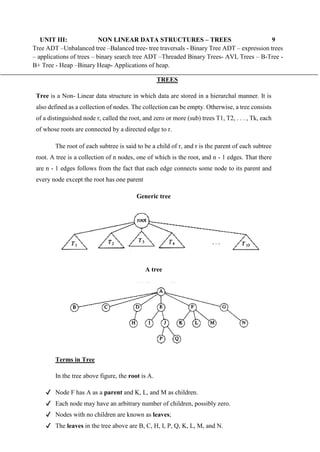
  • 1. UNIT III: NON LINEAR DATA STRUCTURES – TREES 9 Tree ADT –Unbalanced tree –Balanced tree- tree traversals - Binary Tree ADT – expression trees – applications of trees – binary search tree ADT –Threaded Binary Trees- AVL Trees – B-Tree - B+ Tree - Heap –Binary Heap- Applications of heap. TREES Tree is a Non- Linear data structure in which data are stored in a hierarchal manner. It is also defined as a collection of nodes. The collection can be empty. Otherwise, a tree consists of a distinguished node r, called the root, and zero or more (sub) trees T1, T2, . . . , Tk, each of whose roots are connected by a directed edge to r. The root of each subtree is said to be a child of r, and r is the parent of each subtree root. A tree is a collection of n nodes, one of which is the root, and n - 1 edges. That there are n - 1 edges follows from the fact that each edge connects some node to its parent and every node except the root has one parent Generic tree A tree Terms in Tree In the tree above figure, the root is A. ✔ Node F has A as a parent and K, L, and M as children. ✔ Each node may have an arbitrary number of children, possibly zero. ✔ Nodes with no children are known as leaves; ✔ The leaves in the tree above are B, C, H, I, P, Q, K, L, M, and N.
  • 2. ✔ Nodes with the same parent are siblings; thus K, L, and M are all siblings. Grandparent and grandchild relations can be defined in a similar manner. ✔ A path from node n1 to nk is defined as a sequence of nodes n1, n2, . . . , nk such that ni is the parent of ni+1 for 1 i < k. ✔ The length of this path is the number of edges on the path, namely k -1. ✔ There is a path of length zero from every node to itself. ✔ For any node ni, the depth of ni is the length of the unique path from the root to ni. Thus, the root is at depth 0. ✔ The height of ni is the longest path from ni to a leaf. Thus all leaves are at height 0. ✔ The height of a tree is equal to the height of the root. Example: For the above tree, E is at depth 1 and height 2; F is at depth 1 and height 1; the height of the tree is 3. T Note: ✔ The depth of a tree is equal to the depth of the deepest leaf; this is always equal to the height of the tree. ✔ If there is a path from n1 to n2, then n1 is an ancestor of n2 and n2 is a descendant of n1. If n1 n2, then n1 is a proper ancestor of n2 and n2 is a proper descendant of n1. ✔ A tree there is exactly one path from the root to each node. Types of the Tree Based on the no. of children for each node in the tree, it is classified into two to types. 1. Binary tree 2. General tree Binary tree In a tree, each and every node has a maximum of two children. It can be empty, one or two. Then it is called as Binary tree.
  • 3. Eg: General Tree In a tree, node can have any no of children. Then it is called as general Tree. Eg: Implementation of Trees Tree can be implemented by two methods. 1. Array Implementation 2. Linked List implementation Apart from these two methods, it can also be represented by First Child and Next sibling Representation. One way to implement a tree would be to have in each node, besides its data, a pointer to each child of the node. However, since the number of children per node can vary so greatly and is not known in advance, it might be infeasible to make the children direct links in the data structure, because there would be too much wasted space. The solution is simple: Keep the children of each node in a linked list of tree nodes. Node declarations for trees typedef struct tree_node *tree_ptr; struct tree_node {
  • 4. element_type element; tree_ptr first_child; tree_ptr next_sibling; }; First child/next sibling representation of the tree shown in the below Figure Arrows that point downward are first_child pointers. Arrows that go left to right are next_sibling pointers. Null pointers are not drawn, because there are too many. In the above tree, node E has both a pointer to a sibling (F) and a pointer to a child (I), while some nodes have neither. Tree Traversals Visiting of each and every node in a tree exactly only once is called as Tree traversals. Here Left subtree and right subtree are traversed recursively. Types of Tree Traversal: 1. Inorder Traversal 2. Preorder Traversal 3. Postorder Traversal Inorder traversal: Rules: ● Traverse Left subtree recursively ● Process the node ● Traverse Right subtree recursively
  • 5. Eg Inorder traversal: a + b*c + d*e + f*g. Preorder traversal: Rules: ● Process the node ● Traverse Left subtree recursively ● Traverse Right subtree recursively Preorder traversal: ++a*b c*+*d e f g Postorder traversal: Rules: ● Traverse Left subtree recursively ● Traverse Right subtree recursively ● Process the node Postorder traversal: a b c*+de*f + g* + Tree Traversals with an Application There are many applications for trees. Most important two applications are, 1. Listing a directory in a hierarchical file system 2. Calculating the size of a directory 1. Listing a directory in a hierarchical file system
  • 6. One of the popular uses is the directory structure in many common operating systems, including UNIX, VAX/VMS, and DOS. Typical directories in the UNIX file system (UNIX directory) ✔ The root of this directory is /usr. (The asterisk next to the name indicates that /usr is itself a directory.) ✔ /usr has three children, mark, alex, and bill, which are themselves directories. Thus, /usr contains three directories and no regular files. ✔ The filename /usr/mark/book/ch1.r is obtained by following the leftmost child three times. Each / after the first indicates an edge; the result is the full pathname. ✔ Two files in different directories can share the same name, because they must have different paths from the root and thus have different pathnames. ✔ A directory in the UNIX file system is just a file with a list of all its children, so the directories are structured almost exactly in accordance with the type declaration. ✔ Each directory in the UNIX file system also has one entry that points to itself and another entry that point to the parent of the directory. Thus, technically, the UNIX file system is not a tree, but is treelike. Routine to list a directory in a hierarchical file system void list_directory ( Directory_or_file D ) { list_dir ( D, 0 ); } Void list_dir ( Directory_or_file D, unsigned int depth )
  • 7. { if ( D is a legitimate entry) { print_name ( depth, D ); if( D is a directory ) for each child, c, of D list_dir( c, depth+1 ); } } The logic of the algorithm is as follow. ✔ The argument to list_dir is some sort of pointer into the tree. As long as the pointer is valid, the name implied by the pointer is printed out with the appropriate number of tabs. ✔ If the entry is a directory, then we process all children recursively, one by one. These children are one level deeper, and thus need to be indenting an extra space. This traversal strategy is known as a preorder traversal. In a preorder traversal, work at a node is performed before (pre) its children are processed. If there are n file names to be output, then the running time is O (n). 2. Calculating the size of a directory As above UNIX Directory Structure, the numbers in parentheses representing the number of disk blocks taken up by each file, since the directories are themselves files, they have sizes too. Suppose we would like to calculate the total number of blocks used by all the files in the tree. Here the work at a node is performed after its children are evaluated. So it follows Postorder traversal. The most natural way to do this would be to find the number of blocks contained in the subdirectories /usr/mark (30), /usr/alex (9), and /usr/bill (32). The total number of blocks is then the total in the subdirectories (71) plus the one block used by /usr, for a total of 72. Routine to calculate the size of a directory unsigned
  • 8. int size_directory( Directory_or_file D ) { unsigned int total_size; total_size = 0; if( D is a legitimate entry) { total_size = file_size( D ); if( D is a directory ) for each child, c, of D total_size += size_directory( c ); } return( total_size ); } Binary Trees A binary tree is a tree in which no node can have more than two children. Figure shows that a binary tree consists of a root and two subtrees, Tl and Tr, both of which could possibly be empty. Worst-case binary tree
  • 9. Implementation A binary tree has at most two children; we can keep direct pointers to them. The declaration of tree nodes is similar in structure to that for doubly linked lists, in that a node is a structure consisting of the key information plus two pointers (left and right) to other nodes. Binary tree node declarations typedef struct tree_node *tree_ptr; struct tree_node { element_type element; tree_ptr left; tree_ptr right; }; typedef tree_ptr TREE; Expression Trees When an expression is represented in a binary tree, then it is called as an expression Tree. The leaves of an expression tree are operands, such as constants or variable names, and the other nodes contain operators. It is possible for nodes to have more than two children. It is also possible for a node to have only one child, as is the case with the unary minus operator. We can evaluate an expression tree, T, by applying the operator at the root to the values obtained by recursively evaluating the left and right subtrees. In our example, the left subtree evaluates to a + (b * c) and the right subtree evaluates to ((d *e) + f ) *g. The entire tree therefore represents (a + (b*c)) + (((d * e) + f)* g). We can produce an (overly parenthesized) infix expression by recursively producing a parenthesized left expression, then printing out the operator at the root, and finally recursively producing a parenthesized right expression. This general strattegy ( left, node, right ) is known as an inorder traversal; it gives Infix Expression.
  • 10. An alternate traversal strategy is to recursively print out the left subtree, the right subtree, and then the operator. If we apply this strategy to our tree above, the output is a b c * + d e * f + g * +, which is called as postfix Expression. This traversal strategy is generally known as a postorder traversal. A third traversal strategy is to print out the operator first and then recursively print out the left and right subtrees. The resulting expression, + + a * b c * + * d e f g, is the less useful prefix notation and the traversal strategy is a preorder traversal Expression tree for (a + b * c) + ((d * e + f ) * g) Constructing an Expression Tree Algorithm to convert a postfix expression into an expression tree 1. Read the postfix expression one symbol at a time. 2. If the symbol is an operand, then a. We create a one node tree and push a pointer to it onto a stack. 3. If the symbol is an operator, a. We pop pointers to two trees T1 and T2 from the stack (T1 is popped first) and form a new tree whose root is the operator and whose left and right children point to T2 and T1 respectively. 4. A pointer to this new tree is then pushed onto the stack. Suppose the input is a b + c d e + * *
  • 11. The first two symbols are operands, so we create one-node trees and push pointers to them onto a stack. Next, a '+' is read, so two pointers to trees are popped, a new tree is formed, and a pointer to it is pushed onto the stack. Next, c, d, and e are read, and for each a one-node tree is created and a pointer to the corresponding tree is pushed onto the stack. Now a '+' is read, so two trees are merged. Continuing, a '*' is read, so we pop two tree pointers and form a new tree with a '*' as root. Finally, the last symbol is read, two trees are merged, and a pointer to the final
  • 12. tree is left on the stack. The Search Tree ADT-Binary Search Tree The property that makes a binary tree into a binary search tree is that for every node, X, in the tree, the values of all the keys in the left subtree are smaller than the key value in X, and the values of all the keys in the right subtree are larger than the key value in X. Notice that this implies that all the elements in the tree can be ordered in some consistent manner. In the above figure, the tree on the left is a binary search tree, but the tree on the right is not. The tree on the right has a node with key 7 in the left subtree of a node with key 6. The average depth of a binary search tree is O(log n). Binary search tree declarations typedef struct tree_node *tree_ptr; struct tree_node { element_type element;
  • 13. tree_ptr left; tree_ptr right; }; typedef tree_ptr SEARCH_TREE; Make Empty: This operation is mainly for initialization. Some programmers prefer to initialize the first element as a one-node tree, but our implementation follows the recursive definition of trees more closely. Find This operation generally requires returning a pointer to the node in tree T that has key x, or NULL if there is no such node. The structure of the tree makes this simple. If T is , then we can just return . Otherwise, if the key stored at T is x, we can return T. Otherwise, we make a recursive call on a subtree of T, either left or right, depending on the relationship of x to the key stored in T. Routine to make an empty tree SearchTree makeempty (search tree T) { if(T!=NULL) { Makeempty (T->left); Makeempty (T->Right); Free( T); } return NULL; }
  • 14. Routine for Find operation Position find( Elementtype X, SearchTree T ) { if( T == NULL ) return NULL; if( x < T->element ) return( find( x, T->left ) ); else if( x > T->element ) return( find( x, T->right ) ); else return T; } FindMin & FindMax: These routines return the position of the smallest and largest elements in the tree, respectively. To perform a findmin, start at the root and go left as long as there is a left child. The stopping point is the smallest element. The findmax routine is the same, except that branching is to the right child. Recursive implementation of Findmin for binary search trees Position findmin( SearchTree T ) {
  • 15. if( T == NULL ) return NULL; else if( T->left == NULL ) return( T ); else return( findmin ( T->left ) ); } Recursive implementation of FindMax for binary search trees Position findmax( SearchTree T ) { if( T == NULL ) return NULL; else if( T->Right == NULL ) return( T ); else return( findmax( T->right ) ); } Nonrecursive implementation of FindMin for binary search trees Position findmin( SearchTree T ) { if( T != NULL )
  • 16. while( T->left != NULL ) T=T->left; return(T); } Nonrecursive implementation of FindMax for binary search trees Position findmax( SearchTree T ) { if( T != NULL ) while( T->right != NULL ) T=T->right; return(T); } Insert To insert x into tree T, proceed down the tree. If x is found, do nothing. Otherwise, insert x at the last spot on the path traversed. To insert 5, we traverse the tree as though a find were occurring. At the node with key 4, we need to go right, but there is no subtree, so 5 is not in the tree, and this is the correct spot. Insertion routine Since T points to the root of the tree, and the root changes on the first insertion, insert is written as a function that returns a pointer to the root of the new tree.
  • 17. searchTree insert( elementtype x, SearchTree T ) { if( T == NULL ) { T = (SEARCH_TREE) malloc ( sizeof (struct tree_node) ); if( T == NULL ) fatal_error("Out of space!!!"); else { T->element = x; T->left = T->right = NULL; } } else if( x < T->element ) T->left = insert( x, T->left ); else if( x > T->element ) T->right = insert( x, T->right ); /* else x is in the tree already. We'll do nothing */ return T; } Delete Once we have found the node to be deleted, we need to consider several possibilities. If the node is a leaf, it can be deleted immediately.
  • 18. If the node has one child, the node can be deleted after its parent adjusts a pointer to bypass the node if a node with two children. The general strategy is to replace the key of this node with the smallest key of the right subtree and recursively delete that node. Because the smallest node in the right subtree cannot have a left child, the second delete is an easy one. The node to be deleted is the left child of the root; the key value is 2. It is replaced with the smallest key in its right subtree (3), and then that node is deleted as before. Deletion of a node (4) with one child, before and after Deletion of a node (2) with two children, before and after If the number of deletions is expected to be small, then a popular strategy to use is lazy deletion: When an element is to be deleted, it is left in the tree and merely marked as being deleted.
  • 19. Deletion routine for binary search trees Searchtree delete( elementtype x, searchtree T ) { Position tmpcell; if( T == NULL ) error("Element not found"); else if( x < T->element ) /* Go left */ T->left = delete( x, T->left ); else if( x > T->element ) /* Go right */ T->right = delete( x, T->right ); else /* Found element to be deleted */ if( T->left && T->right ) /* Two children */ { tmp_cell = find_min( T->right ); T->element = tmp_cell->element; T->right = delete( T->element, T->right ); } else /* One child */ { tmpcell = T; if( T->left == NULL ) /* Only a right child */ T= T->right;
  • 20. if( T->right == NULL ) /* Only a left child */ T = T->left; free( tmpcell ); } return T; } Average-Case Analysis of BST ✔ All of the operations of the previous section, except makeempty, should take O(log n) time, because in constant time we descend a level in the tree, thus operating on a tree that is now roughly half as large. ✔ The running time of all the operations, except makeempty is O(d), where d is the depth of the node containing the accessed key. ✔ The average depth over all nodes in a tree is O(log n). ✔ The sum of the depths of all nodes in a tree is known as the internal path length. Threaded Binary Tree ● A binary tree is threaded by making all right child pointers that would normally be null point to the inorder successor of the node (if it exists), and all left child pointers that would normally be null point to the inorder predecessor of the node. ● We have the pointers reference the next node in an inorder traversal; called threads ● We need to know if a pointer is an actual link or a thread, so we keep a boolean for each pointer Why do we need Threaded Binary Tree? ● Binary trees have a lot of wasted space: the leaf nodes each have 2 null pointers. We can use these pointers to help us in inorder traversals. ● Threaded binary tree makes the tree traversal faster since we do not need stack or recursion for traversal Types of threaded binary trees: ● Single Threaded: each node is threaded towards either the in-order predecessor or successor (left orright) means all right null pointers will point to inorder successor OR all left null pointers will point to inorder predecessor. ● Double threaded: each node is threaded towards both the in-order predecessor and successor (left andright) means all right null pointers will point to inorder successor AND all left null pointers will point to inorder predecessor.
  • 21. Single Threaded: each node is threaded towards either the in-order predecessor or successor (left or right) means all right null pointers will point to inorder successor OR all left null pointers will point to inorder predecessor. Implementation: Let’s see how the Node structure will look like class Node{ Node left; Node right; int data; boolean rightThread; public Node(int data){ this.data = data; rightThread = false; } } In normal BST node we have left and right references and data but in threaded binary tree we have boolean another field called “rightThreaded”. This field will tell whether node’s right pointer is pointing to its inorder successor, but how, we will see it further. Operations: We will discuss two primary operations in single threaded binary tree 1. Insert node into tree 2. Print or traverse the tree.( here we will see the advantage of threaded tree) Insert(): The insert operation will be quite similar to Insert operation in Binary search tree with few modifications. ● To insert a node our first task is to find the place to insert the node.
  • 22. ● Take current = root . ● start from the current and compare root.data with n. ● Always keep track of parent node while moving left or right. ● if current.data is greater than n that means we go to the left of the root, if after moving to left, the current = null then we have found the place where we will insert the new node. Add the new node to the left of parent node and make the right pointer points to parent node and rightThread = true for new node. ● ● if current.data is smaller than n that means we need to go to the right of the root, while going into the right subtree, check rightThread for current node, means right thread is provided and points to the in order successor, if rightThread = false then and current reaches to null, just insert the new node else if rightThread = true then we need to detach the right pointer (store the reference, new node right reference will be point to it) of current node and make it point to the new node and make the right reference point to stored reference. (See image and code for better understanding) Traverse(): traversing the threaded binary tree will be quite easy, no need of any recursion or any stack for storing the node. Just go to the left most node and start traversing the tree using right pointer and whenever rightThread = false again go to the left most node in right subtree. (See image and code for better understanding)
  • 23. Double threaded: Each node is threaded towards both the in-order predecessor and successor (left and right) means all right null pointers will point to inorder successor AND all left null pointers will point to inorder predecessor. Implementation: Let’s see how the Node structure will look like class Node { int data; int leftBit; int rightBit; Node left; Node right; public Node(int data) { this.data = data; } } If you notice we have two extra fields in the node than regular binary tree node. leftBit and rightBit. Let’s see what these fields represent. leftBit=0 left reference points to the inorder predecessor leftBit=1 left reference points to the left child rightBit=0 right reference points to the inorder successor righBit=1 right reference points to the right child Let’s see why do we need these fields and why do we need a dummy node when If we try to convert the normal binary tree to threaded binary Now if you see the picture above , there are two references left most reference and right most reference pointers has nowhere to point to. Need of a Dummy Node: As we saw that references left most reference and right most reference pointers has nowhere to point to so we need a dummy node and this node will
  • 24. always present even when tree is empty. In this dummy node we will put rightBit = 1 and its right child will point to it self and leftBit = 0, so we will construct the threaded tree as the left child of dummy node. Let’s see how the dummy node will look like: Now we will see how this dummy node will solve our problem of references left most reference and right most reference pointers has nowhere to point to. Double Threaded binary tree with dummy node Now we will see the some operations in double threaded binary tree. Insert(): The insert operation will be quite similar to Insert operation in Binary search tree with few modifications. 1. To insert a node our first task is to find the place to insert the node. 2. First check if tree is empty, means tree has just dummy node then then insert the new node into left subtree of the dummy node. 3. If tree is not empty then find the place to insert the node, just like in normal BST. 4. If new node is smaller than or equal to current node then check if leftBit =0, if yes then we have found the place to insert the node, it will be in the left of the subtree and if leftBit=1 then go left. 5. If new node is greater than current node then check if rightBit =0, if yes then we have found the place to insert the node, it will be in the right of the subtree and if rightBit=1 then go right. 6. Repeat step 4 and 5 till the place to be inserted is not found. 7. Once decided where the node will be inserted, next task would be to insert the node. first we will see how the node will be inserted as left child. n.left = current.left; current.left = n;
  • 25. n.leftBit = current.leftBit; current.leftBit = 1; n.right = current; see the image below for better understanding 8. To insert the node as right child. n.right = current.right; current.right = n; n.rightBit = current.rightBit; current.rightBit = 1; n.left = current; see the image below for better understanding.
  • 26. Traverse(): Now we will see how to traverse in the double threaded binary tree, we do not need a recursion to do that which means it won’t require stack, it will be done n one single traversal in O(n). Starting from left most node in the tree, keep traversing the inorder successor and print it.(click here to read more about inorder successor in a tree). See the image below for more understanding. AVL Trees The balance condition and allow the tree to be arbitrarily deep, but after every operation, a restructuring rule is applied that tends to make future operations efficient. These types of data structures are generally classified as self-adjusting. An AVL tree is identical to a binary search tree, except that for every node in the tree, the height of the left and right subtrees can differ by at most 1. (The height of an empty tree is defined to be -1.) An AVL (Adelson-Velskii and Landis) tree is a binary search tree with a balance condition. The simplest idea is to require that the left and right subtrees have the same height. The balance condition must be easy to maintain, and it ensures that the depth of the tree is O(log n).
  • 27. The above figure shows, a bad binary tree. Requiring balance at the root is not enough. In Figure, the tree on the left is an AVL tree, but the tree on the right is not. Thus, all the tree operations can be performed in O(log n) time, except possibly insertion. When we do an insertion, we need to update all the balancing information for the nodes on the path back to the root, but the reason that insertion is difficult is that inserting a node could violate the AVL tree property. Inserting a node into the AVL tree would destroy the balance condition. Let us call the unbalanced node α. Violation due to insertion might occur in four cases: 1. An insertion into the left subtree of the left child of α 2. An insertion into the right subtree of the left child of α 3. An insertion into the left subtree of the right child of α 4. An insertion into the right subtree of the right child of α Violation of AVL property due to insertion can be avoided by doing some modification on the node α. This modification process is called as Rotation. Types of rotation 1. Single Rotation 2. Double Rotation
  • 28. Single Rotation (case 1) – Single rotate with Left The two trees in the above Figure contain the same elements and are both binary search trees. First of all, in both trees k1 < k2. Second, all elements in the subtree X are smaller than k1 in both trees. Third, all elements in subtree Z are larger than k2. Finally, all elements in subtree Y are in between k1 and k2. The conversion of one of the above trees to the other is known as a rotation. In an AVL tree, if an insertion causes some node in an AVL tree to lose the balance property: Do a rotation at that node. The basic algorithm is to start at the node inserted and travel up the tree, updating the balance information at every node on the path. In the above figure, after the insertion of the in the original AVL tree on the left, node 8 becomes unbalanced. Thus, we do a single rotation between 7 and 8, obtaining the tree on the right. Routine : Static position Singlerotatewithleft( Position K2) {
  • 29. Position k1; K1=k2->left; K2->left=k1->right; K1->right=k2; K2->height=max(height(k2->left),height(k2->right)); K1->height=max(height(k1->left),k2->height); Return k1; } Single Rotation (case 4) – Single rotate with Right (Refer diagram from Class note) Suppose we start with an initially empty AVL tree and insert the keys 1 through 7 in sequential order. The first problem occurs when it is time to insert key 3, because the AVL property is violated at the root. We perform a single rotation between the root and its right child to fix the problem. The tree is shown in the following figure, before and after the rotation. A dashed line indicates the two nodes that are the subject of the rotation. Next, we insert the key 4, which causes no problems, but the insertion of 5 creates a violation at node 3, which is fixed by a single rotation. Next, we insert 6. This causes a balance problem for the root, since its left subtree is of height 0, and its right subtree would be height 2. Therefore, we perform a single rotation at the root between 2 and 4.
  • 30. The rotation is performed by making 2 a child of 4 and making 4's original left subtree the new right subtree of 2. Every key in this subtree must lie between 2 and 4, so this transformation makes sense. The next key we insert is 7, which causes another rotation. Routine : Static position Singlerotatewithright( Position K1) { Position k2; K2=k1->right; K1->right=k2->left; K2->left=k1;
  • 32. In the above diagram, suppose we insert keys 8 through 15 in reverse order. Inserting 15 is easy, since it does not destroy the balance property, but inserting 14 causes a height imbalance at node 7. As the diagram shows, the single rotation has not fixed the height imbalance. The problem is that the height imbalance was caused by a node inserted into the tree containing the middle elements (tree Y in Fig. (Right-left) double rotation) at the same time as the other trees had identical heights. This process is called as double rotation, which is similar to a single rotation but involves four subtrees instead of three.
  • 33. In our example, the double rotation is a right-left double rotation and involves 7, 15, and 14. Here, k3 is the node with key 7, k1 is the node with key 15, and k2 is the node with key 14. Next we insert 13, which require a double rotation. Here the double rotation is again a right-left double rotation that will involve 6, 14, and 7 and will restore the tree. In this case, k3 is the node with key 6, k1 is the node with key 14, and k2 is the node with key 7. Subtree A is the tree rooted at the node with key 5, subtree B is the empty subtree that was originally the left child of the node with key 7, subtree C is the tree rooted at the node with key 13, and finally, subtree D is the tree rooted at the node with key 15. If 12 is now inserted, there is an imbalance at the root. Since 12 is not between
  • 34. 4 and 7, we know that the single rotation will work. Insertion of 11 will require a single rotation: To insert 10, a single rotation needs to be performed, and the same is true for the subsequent insertion of 9. We insert 8 without a rotation, creating the almost perfectly balanced tree. Routine for double Rotation with left (Case 2) Static position doublerotatewithleft(position k3) { K3->left=singlerotatewithright(k3->left); Return singlerotatewithleft(k3); } Routine for double Rotation with right (Case 3) Static position doublerotatewithlright(position k1) { K1->right=singlerotatewithleft(k1->right); Return singlerotatewithright(k1); } Node declaration for AVL trees: typedef struct avlnode *position; typedef struct avlnode *avltree; struct avlnode
  • 35. { elementtype element; avltree left; avltree right; int height; }; typedef avl_ptr SEARCH_TREE; Routine for finding height of an AVL node Int height (avltree p) { if( p == NULL ) return -1; else return p->height; } Routine for insertion of new element into a AVL TREE (Refer Class note) B-Trees AVL tree and Splay tree are binary; there is a popular search tree that is not binary. This tree is known as a B-tree. A B-tree of order m is a tree with the following structural properties: a. The root is either a leaf or has between 2 and m children. b. All nonleaf nodes (except the root) have between m/2 and m children. c. All leaves are at the same depth. All data is stored at the leaves. Contained in each interior node are pointers p1, p2, . . . , pm to the children, and values k1, k2, . . . , km - 1, representing the smallest key
  • 36. found in the subtrees p2, p3, . . . , pm respectively. Some of these pointers might be NULL, and the corresponding ki would then be undefined. For every node, all the keys in subtree p1 are smaller than the keys in subtree p2, and so on. The leaves contain all the actual data, which is either the keys themselves or pointers to records containing the keys. The number of keys in a leaf is also between m/2 and m. An example of a B-tree of order 4 A B-tree of order 4 is more popularly known as a 2-3-4 tree, and a B-tree of order 3 is known as a 2-3 tree Our starting point is the 2-3 tree that follows.
  • 37. We have drawn interior nodes (nonleaves) in ellipses, which contain the two pieces of data for each node. A dash line as a second piece of information in an interior node indicates that the node has only two children. Leaves are drawn in boxes, which contain the keys. The keys in the leaves are ordered. To perform a find, we start at the root and branch in one of (at most) three directions, depending on the relation of the key we are looking for to the two values stored at the node. When we get to a leaf node, we have found the correct place to put x. Thus, to insert a node with key 18, we can just add it to a leaf without causing any violations of the 2-3 tree properties. The result is shown in the following figure. If we now try to insert 1 into the tree, we find that the node where it belongs is already full. Placing our new key into this node would give it a fourth element which is not allowed. This can be solved by making two nodes of two keys each and adjusting the information in the parent.
  • 38. To insert 19 into the current tree, two nodes of two keys each, we obtain the following tree. This tree has an internal node with four children, but we only allow three per node. Again split this node into two nodes with two children. Now this node might be one of three children itself, and thus splitting it would create a problem for its parent but we can keep on splitting nodes on the way up to the root until we either get to the root or find a node with only two children. If we now insert an element with key 28, we create a leaf with four children, which is split into two leaves of two children.
  • 39. This creates an internal node with four children, which is then split into two children. Like to insert 70 into the tree above, we could move 58 to the leaf containing 41 and 52, place 70 with 59 and 61, and adjust the entries in the internal nodes. Deletion in B-Tree ● If this key was one of only two keys in a node, then its removal leaves only one key. We can fix this by combining this node with a sibling. If the sibling has three keys, we can steal one and have both nodes with two keys. ● If the sibling has only two keys, we combine the two nodes into a single node with three keys. The parent of this node now loses a child, so we might have to percolate this strategy all the way to the top. ● If the root loses its second child, then the root is also deleted and the tree becomes one level shallower. We repeat this until we find a parent with less than m children. If we split the root, we create a new root with two children. The depth of a B-tree is at most log m/2 n. The worst-case running time for each of the insert and delete operations is thus O(m logm n) = O( (m / log m ) log n), but a find takes only O(log n ).
  • 40. B+ Tree ● B+ Tree is an extension of B Tree which allows efficient insertion, deletion and search operations. ● In B Tree, Keys and records both can be stored in the internal as well as leaf nodes. Whereas, in B+ tree, records (data) can only be stored on the leaf nodes while internal nodes can only store the key values. ● The leaf nodes of a B+ tree are linked together in the form of a singly linked lists to make the search queries more efficient. ● B+ Tree are used to store the large amount of data which can not be stored in the main memory. Due to the fact that, size of main memory is always limited, the internal nodes (keys to access records) of the B+ tree are stored in the main memory whereas, leaf nodes are stored in the secondary memory. ● The internal nodes of B+ tree are often called index nodes. A B+ tree of order 3 is shown in the following figure. B+ Tree Advantages of B+ Tree ● Records can be fetched in equal number of disk accesses. ● Height of the tree remains balanced and less as compare to B tree. ● We can access the data stored in a B+ tree sequentially as well as directly. ● Keys are used for indexing. ● Faster search queries as the data is stored only on the leaf nodes. B Tree VS B+ Tree S.NO B Tree B+ Tree
  • 41. 1 Search keys can not be repeatedly stored. Redundant search keys can be present. 2 Data can be stored in leaf nodes as well as internal nodes Data can only be stored on the leaf nodes. 3 Searching for some data is a slower process since data can be found on internal nodes as well as on the leaf nodes. Searching is comparatively faster as data can only be found on the leaf nodes. 4 Deletion of internal nodes are so complicated and time consuming. Deletion will never be a complexed process since element will always be deleted from the leaf nodes. 5 Leaf nodes can not be linked together. Leaf nodes are linked together to make the search operations more efficient. Insertion in B+ Tree Step 1: Insert the new node as a leaf node Step 2: If the leaf doesn't have required space, split the node and copy the middle node to the next index node. Step 3: If the index node doesn't have required space, split the node and copy the middle element to the next index page. Example : Insert the value 195 into the B+ tree of order 5 shown in the following figure. 195 will be inserted in the right sub-tree of 120 after 190. Insert it at the desired position. The node contains greater than the maximum number of elements i.e. 4, therefore split it and place the median node up to the parent. Now, the index node contains 6 children and 5 keys which violates the B+ tree properties, therefore we need to split it, shown as follows.
  • 42. Deletion in B+ Tree Step 1: Delete the key and data from the leaves. Step 2: if the leaf node contains less than minimum number of elements, merge down the node with its sibling and delete the key in between them. Step 3: if the index node contains less than minimum number of elements, merge the node with the sibling and move down the key in between them. Example Delete the key 200 from the B+ Tree shown in the following figure. 200 is present in the right sub-tree of 190, after 195. delete it. Merge the two nodes by using 195, 190, 154 and 129. Now, element 120 is the single element present in the node which is violating the B+ Tree
  • 43. properties. Therefore, we need to merge it by using 60, 78, 108 and 120. Now, the height of B+ tree will be decreased by 1. PRIORITY QUEUES (HEAPS) A queue is said to be priority queue, in which the elements are dequeued based on the priority of the elements. A priority queue is used in, ● Jobs sent to a line printer are generally placed on a queue. For instance, one job might be particularly important, so that it might be desirable to allow that job to be run as soon as the printer is available. ● In a multiuser environment, the operating system scheduler must decide which of several processes to run. Generally a process is only allowed to run for a fixed period of time. One algorithm uses a queue. Jobs are initially placed at the end of the queue. The scheduler will repeatedly take the first job on the queue, run it until either it finishes or its time limit is up, and place it at the end of the queue. This strategy is generally not appropriate, because very short jobs will seem to take a long time because of the wait involved to run. Generally, it is important that short jobs finish as fast as possible. This is called as Shortest Job First (SJF). This particular application seems to require a special kind of queue, known as a priority queue. Basic model of a priority queue A priority queue is a data structure that allows at least the following two operations: 1. Insert, equivalent of enqueue 2. Deletemin, removes the minimum element in the heap equivalent of the Queue’s dequeue operation. Implementations of Priority Queue 1. Array Implementation 2. Linked list Implementation 3. Binary Search Tree implementation 4. Binary Heap Implementation Array Implementation
  • 44. Drawbacks: 1. There will be more wastage of memory due to maximum size of the array should be define in advance 2. Insertion taken at the end of the array which takes O (N) time. 3. Delete_min will also take O (N) times.
  • 45. Linked list Implementation It overcomes first two problems in array implementation. But delete_min operation takes O(N) time similar to array implementation. Binary Search Tree implementation Another way of implementing priority queues would be to use a binary search tree. This gives an O(log n) average running time for both operations. Binary Heap Implementation Another way of implementing priority queues would be to use a binary heap. This gives an O(1) average running time for both operations. Binary Heap Like binary search trees, heaps have two properties, namely, a structure property and a heap order property. As with AVL trees, an operation on a heap can destroy one of the properties, so a heap operation must not terminate until all heap properties are in order. 1. Structure Property 2. Heap Order Property Structure Property A heap is a binary tree that is completely filled, with the possible exception of the bottom level, which is filled from left to right. Such a tree is known as a complete binary tree. A complete Binary Tree A complete binary tree of height h has between 2h and 2h+1 - 1 nodes. This implies that the height of a complete binary tree is log n, which is clearly O(log n).
  • 46. Array implementation of complete binary tree Note: For any element in array position i, the left child is in position 2i, the right child is in the cell after the left child (2i + 1), and the parent is in position i/2 . The only problem with this implementation is that an estimate of the maximum heap size is required in advance. Types of Binary Heap Min Heap A binary heap is said to be Min heap such that any node x in the heap, the key value of X is smaller than all of its descendants children. Max Heap A binary heap is said to be Min heap such that any node x in the heap, the key value of X is larger than all of its descendants children.
  • 47. It is easy to find the minimum quickly, it makes sense that the smallest element should be at the root. If we consider that any subtree should also be a heap, then any node should be smaller than all of its descendants. Applying this logic, we arrive at the heap order property. In a heap, for every node X, the key in the parent of X is smaller than (or equal to) the key in X. Similarly we can declare a (max) heap, which enables us to efficiently find and remove the maximum element, by changing the heap order property. Thus, a priority queue can be used to find either a minimum or a maximum. By the heap order property, the minimum element can always be found at the root. Declaration for priority queue struct heapstruct { int capacity; int size; element_type *elements; }; typedef struct heapstruct *priorityQ; Create routine of priority Queue priorityQ create (int max_elements )
  • 48. { priorityQ H; if( max_elements < MIN_PQ_SIZE ) error("Priority queue size is too small"); H = (priorityQ) malloc ( sizeof (struct heapstruct) ); if( H == NULL ) fatal_error("Out of space!!!"); H->elements = (element_type *) malloc( ( max_elements+1) * sizeof (element_type) ); if( H->elements == NULL ) fatal_error("Out of space!!!"); H->capacity= max_elements; H->size = 0; H->elements[0] = MIN_DATA; return H; } Basic Heap Operations It is easy to perform the two required operations. All the work involves ensuring that the heap order property is maintained. 1. Insert 2. Deletemi n Insert To insert an element x into the heap, we create a hole in the next available location, since otherwise the tree will not be complete. If x can be placed in the hole without violating heap order, then we do so and are done. Otherwise we slide the element that is in the hole's parent node into the hole, thus bubbling the hole up toward the root. We continue this process until x can be placed in the hole.
  • 49. Figure shows that to insert 14, we create a hole in the next available heap location. Inserting 14 in the hole would violate the heap order property, so 31 is slide down into the hole. This strategy is continued until the correct location for 14 is found. This general strategy is known as a percolate up; the new element is percolated up the heap until the correct location is found. We could have implemented the percolation in the insert routine by performing repeated swaps until the correct order was established, but a swap requires three assignment statements. If an element is percolated up d levels, the number of assignments performed by the swaps would be 3d. Our method uses d + 1 assignments. Routine to insert into a binary heap /* H->element[0] is a sentinel */ Void insert( element_type x, priorityQ H ) { int i; if( is_full( H ) )
  • 50. error("Priority queue is full"); else { i = ++H->size; while( H->elements[i/2] > x ) { H->elements[i] = H->elements[i/2]; i /= 2; } H->elements[i] = x; } } If the element to be inserted is the new minimum, it will be pushed all the way to the top. The time to do the insertion could be as much as O (log n), if the element to be inserted is the new minimum and is percolated all the way to the root. On Deletemin Deletemin are handled in a similar manner as insertions. Finding the minimum is easy; the hard part is removing it. When the minimum is removed, a hole is created at the root. Since the heap now becomes one smaller, it follows that the last element x in the heap must move somewhere in the heap. If x can be placed in the hole, then we are done. This is unlikely, so we slide the smaller of the hole's children into the hole, thus pushing the hole down one level. We repeat this step until x can be placed in the hole. This general strategy is known as a percolate down.
  • 51. In Figure, after 13 is removed, we must now try to place 31 in the heap. 31 cannot be placed in the hole, because this would violate heap order. Thus, we place the smaller child (14) in the hole, sliding the hole down one level. We repeat this again, placing 19 into the hole and creating a new hole one level deeper. We then place 26 in the hole and create a new hole on the bottom level. Finally, we are able to place 31 in the hole. Routine to perform deletemin in a binary heap element_type delete_min( priorityQ H ) { int i, child; element_type min_element, last_element; if( is_empty( H ) ) { error("Priority queue is empty"); return H->elements[0]; } min_element = H->elements[1];
  • 52. last_element = H->elements[H->size--]; for( i=1; i*2 <= H->size; i=child ) { child = i*2; if( ( child != H->size ) && ( H->elements[child+1] < H->elements [child] ) ) child++; if( last_element > H->elements[child] ) H->elements[i] = H->elements[child]; else break; } H->elements[i] = last_element; return min_element; } The worst-case running time for this operation is O(log n). On average, the element that is placed at the root is percolated almost to the bottom of the heap, so the average running time is O (log n). Other Heap Operations The other heap operations are 1. Decreasekey 2. Increasekey 3. Delete 4. Buildheap Decreasekey The decreasekey(x, ∆, H) operation lowers the value of the key at position x by a positive amount ∆. Since this might violate the heap order, it must be fixed by a percolate up.
  • 53. USE: This operation could be useful to system administrators: they can make their programs run with highest priority. Increasekey The increasekey(x, ∆, H) operation increases the value of the key at position x by a positive amount ∆. This is done with a percolate down. USE: Many schedulers automatically drop the priority of a process that is consuming excessive CPU time. Delete The delete(x, H) operation removes the node at position x from the heap. This is done by first performing decreasekey(x,∆ , H) and then performing deletemin(H). When a process is terminated by a user, it must be removed from the priority queue. Buildheap The buildheap(H) operation takes as input n keys and places them into an empty heap. This can be done with n successive inserts. Since each insert will take O(1) average and O(log n) worst-case time, the total running time of this algorithm would be O(n) average but O(n log n) worst-case.
  • 54. UNIT IV : NON LINEAR DATA STRUCTURES – GRAPHS 9 Definition – Representation of Graph – Types of graph - Breadth-first traversal - Depth-first traversal – Topological Sort – Bi-connectivity – Cut vertex – Euler circuits – Applications of graphs-minimum spanning tree-dijkstra's algorithm-kruskal's algorithm Graph A graph can be defined as group of vertices and edges that are used to connect these vertices. A graph can be seen as a cyclic tree, where the vertices (Nodes) maintain any complex relationship among them instead of having parent child relationship. Definition A graph G can be defined as an ordered set G(V, E) where V(G) represents the set of vertices and E(G) represents the set of edges which are used to connect these vertices. A Graph G(V, E) with 5 vertices (A, B, C, D, E) and six edges ((A,B), (B,C), (C,E), (E,D), (D,B), (D,A)) is shown in the following figure. Directed and Undirected Graph A graph can be directed or undirected. However, in an undirected graph, edges are not associated with the directions with them. An undirected graph is shown in the above figure since its edges are not attached with any of the directions. If an edge exists between vertex A and B then the vertices can be traversed from B to A as well as A to B. In a directed graph, edges form an ordered pair. Edges represent a specific path from some vertex A to another vertex B. Node A is called initial node while node B is called terminal node. A directed graph is shown in the following figure.
  • 55. Graph Terminology Path A path can be defined as the sequence of nodes that are followed in order to reach some terminal node V from the initial node U. Closed Path A path will be called as closed path if the initial node is same as terminal node. A path will be closed path if V0=VN. Simple Path If all the nodes of the graph are distinct with an exception V0=VN, then such path P is called as closed simple path. Cycle A cycle can be defined as the path which has no repeated edges or vertices except the first and last vertices. Connected Graph A connected graph is the one in which some path exists between every two vertices (u, v) in V. There are no isolated nodes in connected graph. Complete Graph A complete graph is the one in which every node is connected with all other nodes. A complete graph contain n(n-1)/2 edges where n is the number of nodes in the graph. Weighted Graph In a weighted graph, each edge is assigned with some data such as length or weight. The weight of an edge e can be given as w(e) which must be a positive (+) value indicating the cost of traversing the edge. Digraph A digraph is a directed graph in which each edge of the graph is associated with some direction and the traversing can be done only in the specified direction.
  • 56. Loop An edge that is associated with the similar end points can be called as Loop. Adjacent Nodes If two nodes u and v are connected via an edge e, then the nodes u and v are called as neighbours or adjacent nodes. Degree of the Node A degree of a node is the number of edges that are connected with that node. A node with degree 0 is called as isolated node. Graph representation In this article, we will discuss the ways to represent the graph. By Graph representation, we simply mean the technique to be used to store some graph into the computer's memory. A graph is a data structure that consist a sets of vertices (called nodes) and edges. There are two ways to store Graphs into the computer's memory: o Sequential representation (or, Adjacency matrix representation) o Linked list representation (or, Adjacency list representation) In sequential representation, an adjacency matrix is used to store the graph. Whereas in linked list representation, there is a use of an adjacency list to store the graph. Representation of Graphs 1. Adjacency matrix / Incidence Matrix 2. Adjacency Linked List/ Incidence Linked List Adjacency matrix We will consider directed graphs. (Fig. 1) Now we can number the vertices, starting at 1. The graph shown in above figure represents 7 vertices and 12 edges. One simple way to represent a graph is to use a two-dimensional array. This is known as an adjacency matrix representation.
  • 57. For each edge (u, v), we set a[u][v]= 1; otherwise the entry in the array is 0. If the edge has a weight associated with it, then we can set a[u][v] equal to the weight and use either a very large or a very small weight as a sentinel to indicate nonexistent edges. Advantage is, it is extremely simple, and the space requirement is (|V|2 ). For directed graph A[u][v]= { 1, if there is edge from u to v 0 otherwise } For undirected graph A[u][v]= { 1, if there is edge between u and v 0 otherwise } For weighted graph A[u][v]= { value , if there is edge from u to v ∞, if no edge between u and v } Adjacency lists Adjacency lists are the standard way to represent graphs. Undirected graphs can be similarly represented; each edge (u, v) appears in two lists, so the space usage essentially doubles. A common requirement in graph algorithms is to find all vertices adjacent to some given vertex v, and this can be done, in time proportional to the number of such vertices found, by a simple scan down the appropriate adjacency list. An adjacency list representation of a graph (See above fig 5.1)
  • 58. Topological Sort A topological sort is an ordering of vertices in a directed acyclic graph, such that if there is a path from vi to vj, then vj appears after vi in the ordering. It is clear that a topological ordering is not possible if the graph has a cycle, since for two vertices v and w on the cycle, v precedes w and w precedes v. Directed acyclic graph In the above graph v1, v2, v5, v4, v3, v7, v6 and v1, v2, v5, v4, v7, v3, v6 are both topological orderings. A simple algorithm to find a topological ordering First, find any vertex with no incoming edges (Source vertex). We can then print this vertex, and remove it, along with its edges, from the graph. To formalize this, we define the indegree of a vertex v as the number of edges (u,v). We compute the indegrees of all vertices in the graph. Assuming that the indegree array is initialized and that the graph is read into an adjacency list, Indegree Before Dequeue # Vertex 1 2 3 4 5 6 7 v1 0 0 0 0 0 0 0 v2 1 0 0 0 0 0 0 v3 2 1 1 1 0 0 0 v4 3 2 1 0 0 0 0
  • 59. v5 1 1 0 0 0 0 0 v6 3 3 3 3 2 1 0 v7 2 2 2 1 0 0 0 Enqueue v1 v2 v5 v4 v3 v7 v6 Dequeue v1 v2 v5 v4 v3 v7 v6 Simple Topological Ordering Routine Void topsort( graph G ) { unsigned int counter; vertex v, w; for( counter = 0; counter < NUM_VERTEX; counter++ ) { v = find_new_vertex_of_indegree_zero( ); if( v = NOT_A_VERTEX ) { error("Graph has a cycle"); break; } top_num[v] = counter; for each w adjacent to v indegree[w]--; }
  • 60. } Explanation The function find_new_vertex_of_indegree_zero scans the indegree array looking for a vertex with indegree 0 that has not already been assigned a topological number. It returns NOT_A_VERTEX if no such vertex exists; this indicates that the graph has a cycle. Routine to perform Topological Sort Void topsort( graph G ) { QUEUE Q; unsigned int counter; vertex v, w; Q = create_queue( NUM_VERTEX ); makeempty( Q ); counter = 0; for each vertex v if( indegree[v] = 0 ) enqueue( v, Q ); while( !isempty( Q ) ) { v = dequeue( Q ); top_num[v] = ++counter; /* assign next number */ for each w adjacent to v if( --indegree[w] = 0 ) enqueue( w, Q );
  • 61. } if( counter != NUMVERTEX ) error("Graph has a cycle"); dispose_queue( Q ); /* free the memory */ } Graph Traversal: Visiting of each and every vertex in the graph only once is called as Graph traversal. There are two types of Graph traversal. 1. Depth First Traversal/ Search (DFS) 2. Breadth First Traversal/ Search (BFS) Depth First Traversal/ Search (DFS) Depth-first search is a generalization of preorder traversal. Starting at some vertex, v, we process v and then recursively traverse all vertices adjacent to v. If this process is performed on a tree, then all tree vertices are systematically visited in a total of O(|E|) time, since |E| = (|V|). We need to be careful to avoid cycles. To do this, when we visit a vertex v, we mark it visited, since now we have been there, and recursively call depth-first search on all adjacent vertices that are not already marked. The two important key points of depth first search 1. If path exists from one node to another node walk across the edge – exploring the edge 2. If path does not exist from one specific node to any other nodes, return to the previous node where we have been before – backtracking
  • 62. Procedure for DFS Starting at some vertex V, we process V and then recursively traverse all the vertices adjacent to V. This process continues until all the vertices are processed. If some vertex is not processed recursively, then it will be processed by using backtracking. If vertex W is visited from V, then the vertices are connected by means of tree edges. If the edges not included in tree, then they are represented by back edges. At the end of this process, it will construct a tree called as DFS tree. Routine to perform a depth-first search void void dfs( vertex v ) { visited[v] = TRUE; for each w adjacent to v if( !visited[w] ) dfs( w ); } The (global) boolean array visited[ ] is initialized to FALSE. By recursively calling the procedures only on nodes that have not been visited, we guarantee that we do not loop indefinitely. * An efficient way of implementing this is to begin the depth-first search at v1. If we need to restart the depth-first search, we examine the sequence vk, vk + 1, . . . for an unmarked vertex,where vk - 1 is the vertex where the last depth-first search was started. An undirected graph
  • 63. Steps to construct depth-first spanning tree a. We start at vertex A. Then we mark A as visited and call dfs(B) recursively. dfs(B) marks B as visited and calls dfs(C) recursively. b. dfs(C) marks C as visited and calls dfs(D) recursively. c. dfs(D) sees both A and B, but both these are marked, so no recursive calls are made. dfs(D) also sees that C is adjacent but marked, so no recursive call is made there, and dfs(D) returns back to dfs(C). d. dfs(C) sees B adjacent, ignores it, finds a previously unseen vertex E adjacent, and thus calls dfs(E). e. dfs(E) marks E, ignores A and C, and returns to dfs(C). f. dfs(C) returns to dfs(B). dfs(B) ignores both A and D and returns. g. dfs(A) ignores both D and E and returns. Depth-first search of the graph ---------> Back edge Tree edge The root of the tree is A, the first vertex visited. Each edge (v, w) in the graph is present in the tree. If, when we process (v, w), we find that w is unmarked, or if, when we process (w, v), we find that v is unmarked, we indicate this with a tree edge. If when we process (v, w), we find that w is already marked, and when processing (w, v), we find that v is already marked, we draw a dashed line, which we will call a back edge, to indicate that this "edge" is not really part of the tree.
  • 64. Breadth First Traversal (BFS) Here starting from some vertex v, and its adjacency vertices are processed. After all the adjacency vertices are processed, then selecting any one the adjacency vertex and process will continue. If the vertex is not visited, then backtracking is applied to visit the unvisited vertex. Routine: void BFS (vertex v) { visited[v]= true; For each w adjacent to v If (!visited[w]) visited[w] = true; } Example of BFS algorithm Now, let's understand the working of BFS algorithm by using an example. In the example given below, there is a directed graph having 7 vertices. In the above graph, minimum path 'P' can be found by using the BFS that will start from Node A and end at Node E. The algorithm uses two queues, namely QUEUE1 and QUEUE2. QUEUE1 holds all the nodes that are to be processed, while QUEUE2 holds all the nodes that are processed and deleted from QUEUE1. Now, let's start examining the graph starting from Node A. Step 1 - First, add A to queue1 and NULL to queue2. 1. QUEUE1 = {A} 2. QUEUE2 = {NULL}
  • 65. Step 2 - Now, delete node A from queue1 and add it into queue2. Insert all neighbors of node A to queue1. 1. QUEUE1 = {B, D} 2. QUEUE2 = {A} Step 3 - Now, delete node B from queue1 and add it into queue2. Insert all neighbors of node B to queue1. 1. QUEUE1 = {D, C, F} 2. QUEUE2 = {A, B} Step 4 - Now, delete node D from queue1 and add it into queue2. Insert all neighbors of node D to queue1. The only neighbor of Node D is F since it is already inserted, so it will not be inserted again. 1. QUEUE1 = {C, F} 2. QUEUE2 = {A, B, D} Step 5 - Delete node C from queue1 and add it into queue2. Insert all neighbors of node C to queue1. 1. QUEUE1 = {F, E, G} 2. QUEUE2 = {A, B, D, C} Step 5 - Delete node F from queue1 and add it into queue2. Insert all neighbors of node F to queue1. Since all the neighbors of node F are already present, we will not insert them again. 1. QUEUE1 = {E, G} 2. QUEUE2 = {A, B, D, C, F} Step 6 - Delete node E from queue1. Since all of its neighbors have already been added, so we will not insert them again. Now, all the nodes are visited, and the target node E is encountered into queue2. 1. QUEUE1 = {G} 2. QUEUE2 = {A, B, D, C, F, E}
  • 66. Difference between DFS & BFS S. No DFS BFS 1 Back tracking is possible from a dead end. Back tracking is not possible. 2 Vertices from which exploration is incomplete are processed in a LIFO order. The vertices to be explored are organized as a FIFO queue. 3 Search is done in one particular direction at the time. The vertices in the same level are maintained parallel. (Left to right) ( alphabetical ordering)
  • 67. Bi-connectivity / Bi connected Graph: An undirected graph is called Biconnected if there are two vertex-disjoint paths between any two vertices. In a Biconnected Graph, there is a simple cycle through any two vertices. By convention, two nodes connected by an edge form a biconnected graph, but this does not verify the above properties. For a graph with more than two vertices, the above properties must be there for it to be Biconnected. Or in other words: A graph is said to be Biconnected if: 1. It is connected, i.e. it is possible to reach every vertex from every other vertex, by a simple path. 2. Even after removing any vertex the graph remains connected. Following are some examples: How to find if a given graph is Biconnected or not? A connected graph is Biconnected if it is connected and doesn’t have any Articulation Point. We mainly need to check two things in a graph. 1. The graph is connected. 2. There is not articulation point in graph. We start from any vertex and do DFS traversal. In DFS traversal, we check if there is any articulation point. If we don’t find any articulation point, then the graph is Biconnected. Finally, we need to check whether all vertices were reachable in DFS or not. If all vertices were not reachable, then the graph is not even connected.
  • 68. Articulation points If a graph is not biconnected, the vertices whose removal would disconnect the graph are known as articulation points. The above graph is not biconnected: C and D are articulation points. The removal of C would disconnect G, and the removal of D would disconnect E and F, from the rest of the graph. Depth-first search provides a linear-time algorithm to find all articulation points in a connected graph. ● First, starting at any vertex, we perform a depth-first search and number the nodes as they are visited. ● For each vertex v, we call this preorder number num (v). Then, for every vertex v in the depth-first search spanning tree, we compute the lowest-numbered vertex, which we call low(v), that is reachable from v by taking zero or more tree edges and then possibly one back edge (in that order). By the definition of low, low (v) is the minimum of 1. num(v) 2. the lowest num(w) among all back edges (v, w) 3. the lowest low(w) among all tree edges (v, w)
  • 69. The first condition is the option of taking no edges, the second way is to choose no tree edges and a back edge, and the third way is to choose some tree edges and possibly a back edge. The depth-first search tree in the above Figure shows the preorder number first, and then the lowest-numbered vertex reachable under the rule described above. The lowest-numbered vertex reachable by A, B, and C is vertex 1 (A), because they can all take tree edges to D and then one back edge back to A and find low value for all other vertices. Depth-first tree that results if depth-first search starts at C To find articulation points, ● The root is an articulation point if and only if it has more than one child, because if it has two children, removing the root disconnects nodes in different subtrees, and if it has only one child, removing the root merely disconnects the root. ● Any other vertex v is an articulation point if and only if v has some child w such that low (w)>= num (v). Notice that this condition is always satisfied at the root;
  • 70. We examine the articulation points that the algorithm determines, namely C and D. D has a child E, and low (E)>= num (D), since both are 4. Thus, there is only one way for E to get to any node above D, and that is by going through D. Similarly, C is an articulation point, because low (G)>= num (C). Routine to assign num to vertices Void assignnum( vertex v ) { vertex w; num[v] = counter++; visited[v] = TRUE; for each w adjacent to v if( !visited[w] ) { parent[w] = v; assignnum ( w ); } } Routine to compute low and to test for articulation Void assignlow( vertex v ) { vertex w; low[v] = num[v]; /* Rule 1 */ for each w adjacent to v {
  • 71. if( num[w] > num[v] ) /* forward edge */ { assignlow( w ); if( low[w] >= num[v] ) printf( "%v is an articulation pointn", v ); low[v] = min( low[v], low[w] ); /* Rule 3 */ } else if( parent[v] != w ) /* back edge */ low[v] = min( low[v], num[w] ); /* Rule 2 */ } } Testing for articulation points in one depth-first search (test for the root is omitted) void findart( vertex v ) { vertex w; visited[v] = TRUE; low[v] = num[v] = counter++; /* Rule 1 */ for each w adjacent to v { if( !visited[w] ) /* forward edge */ { parent[w] = v; findart( w ); if( low[w] >= num[v] ) printf ( "%v is an articulation pointn", v );
  • 72. low[v] = min( low[v], low[w] ); /* Rule */ } else if( parent[v] != w ) /* back edge */ low[v] = min( low[v], num[w] ); /* Rule 2 */ } } Euler Circuits We must find a path in the graph that visits every edge exactly once. If we are to solve the "extra challenge," then we must find a cycle that visits every edge exactly once. This graph problem was solved in 1736 by Euler and marked the beginning of graph theory. The problem is thus commonly referred to as an Euler path or Euler tour or Euler circuit problem, depending on the specific problem statement. Consider the three figures as shown below. A popular puzzle is to reconstruct these figures using a pen, drawing each line exactly once. The pen may not be lifted from the paper while the drawing is being performed. As an extra challenge, make the pen finish at the same point at which it started. Three drawings 1. The first figure can be drawn only if the starting point is the lower left- or right-hand corner, and it is not possible to finish at the starting point.
  • 73. 2. The second figure is easily drawn with the finishing point the same as the starting point. 3. The third figure cannot be drawn at all within the parameters of the puzzle. We can convert this problem to a graph theory problem by assigning a vertex to each intersection. Then the edges can be assigned in the natural manner, as in figure. The first observation that can be made is that an Euler circuit, which must end on its starting vertex, is possible only if the graph is connected and each vertex has an even degree (number of edges). This is because, on the Euler circuit, a vertex is entered and then left. If exactly two vertices have odd degree, an Euler tour, which must visit every edge but need not return to its starting vertex, is still possible if we start at one of the odd-degree vertices and finish at the other. If more than two vertices have odd degree, then an Euler tour is not possible. That is, any connected graph, all of whose vertices have even degree, must have an Euler circuit As an example, consider the graph in The main problem is that we might visit a portion of the graph and return to the starting point prematurely. If all the edges coming out of the start vertex have been used up, then part of the graph is untraversed. The easiest way to fix this is to find the first vertex on this path that has an untraversed edge, and perform another depth-first search. This will give another circuit, which can be spliced into the original. This is continued until all edges have been traversed.
  • 74. Suppose we start at vertex 5, and traverse the circuit 5, 4, 10, 5. Then we are stuck, and most of the graph is still untraversed. The situation is shown in the Figure. We then continue from vertex 4, which still has unexplored edges. A depth-first search might come up with the path 4, 1, 3, 7, 4, 11, 10, 7, 9, 3, 4. If we splice this path into the previous path of 5, 4, 10, 5, then we get a new path of 5, 4, 1, 3, 7 ,4, 11, 10, 7, 9, 3, 4, 10, 5. The graph that remains after this is shown in the Figure The next vertex on the path that has untraversed edges is vertex 3. A possible circuit would then be 3, 2, 8, 9, 6, 3. When spliced in, this gives the path 5, 4, 1, 3, 2, 8, 9, 6, 3, 7, 4, 11, 10, 7, 9, 3, 4, 10, 5. The graph that remains is in the Figure. On this path, the next vertex with an untraversed edge is 9, and the algorithm finds the circuit 9, 12, 10, 9. When this is added to the current path, a circuit of 5, 4, 1, 3, 2, 8, 9, 12, 10, 9, 6, 3, 7, 4, 11, 10, 7, 9, 3, 4, 10, 5 is obtained. As all the edges are traversed, the algorithm terminates with an Euler circuit.
  • 75. Then the Euler Path for the above graph is 5, 4, 1, 3, 2, 8, 9, 12, 10, 9, 6, 3, 7, 4, 11, 10, 7, 9, 3, 4, 10, 5 Cut vertex and edges A cut vertex is a vertex that when removed (with its boundary edges) from a graph creates more components than previously in the graph. A cut edge is an edge that when removed (the vertices stay in place) from a graph creates more components than previously in the graph. Find the cut vertices and cut edges for the following graphs Answers 31) The cut vertex is c. There are no cut edges. 32) The cut vertices are c and d. The cut edge is (c,d) 33) The cut vertices are b,c,e and i. The cut edges are: (a,b),(b,c),(c,d),(c,e),(e,i),(i,h) Applications of graph: Minimum Spanning Tree Definition: A minimum spanning tree exists if and only if G is connected. A minimum spanning tree of an undirected graph G is a tree formed from graph edges that connects all the vertices of G at lowest total cost.
  • 76. The number of edges in the minimum spanning tree is |V| - 1. The minimum spanning tree is a tree because it is acyclic, it is spanning because it covers every edge. Application: ● House wiring with a minimum length of cable, reduces cost of the wiring. A graph G and its minimum spanning tree There are two algorithms to find the minimum spanning tree 1. Prim's Algorithm 2. Kruskal's Algorithm Kruskal's Algorithm A second greedy strategy is continually to select the edges in order of smallest weight and accept an edge if it does not cause a cycle. Formally, Kruskal's algorithm maintains a forest. Forest is a collection of trees. Procedure ● Initially, there are |V| single-node trees. ● Adding an edge merges two trees into one.
  • 77. ● When the algorithm terminates, there is only one tree, and this is the minimum spanning tree. ● The algorithm terminates when enough edges are accepted. At any point in the process, two vertices belong to the same set if and only if they are connected in the current spanning forest. Thus, each vertex is initially in its own set. ● If u and v are in the same set, the edge is rejected, because since they are already connected, adding (u, v) would form a cycle. ● Otherwise, the edge is accepted, and a union is performed on the two sets containing u and v. Action of Kruskal's algorithm on G Edge Weight Action (v1,v4) 1 Accepted (v6,v7) 1 Accepted (v1,v2) 2 Accepted (v3,v4) 2 Accepted (v2,v4) 3 Rejected (v1,v3) 4 Rejected (v4,v7) 4 Accepted (v3,v6) 5 Rejected (v5,v7) 6 Accepted
  • 78. Kruskal's algorithm after each stage Routine for Kruskal's algorithm void Graph:: kruskal( ) { int edgesaccepted = 0; DISJSET ds ( Numvertex); PRIORIT_QUEUE < edge> pg( getedges ( )); Edge e; Vertex U, V; while( edgesaccepted < NUMVERTEX-1 ) { Pq. deletemin( e ); // e = (u, v) Settype Uset =ds. find( U, S ); Settype Vset = ds.find( V, S );
  • 79. if( Uset != Vset ) { // accept the edge edgesaccepted++; ds.setunion( S, Uset, Vset ); } } } Dijkstra's Algorithm: ● It is a greedy algorithm that solves the single-source shortest path problem for a directed graph G = (V, E) with nonnegative edge weights, i.e., w (u, v) ≥ 0 for each edge (u, v) ∈ E. ● Dijkstra's Algorithm maintains a set S of vertices whose final shortest - path weights from the source s have already been determined. That's for all vertices v ∈ S; we have d [v] = δ (s, v). The algorithm repeatedly selects the vertex u ∈ V - S with the minimum shortest - path estimate, insert u into S and relaxes all edges leaving u. ● Because it always chooses the "lightest" or "closest" vertex in V - S to insert into set S, it is called as the greedy strategy. Dijkstra's Algorithm (G, w, s) INITIALIZE - SINGLE - SOURCE (G, s) S←∅ Q←V [G] while Q ≠ ∅ do u ← EXTRACT - MIN (Q) S ← S ∪ {u} for each vertex v ∈ Adj [u] do RELAX (u, v, w) Following are the steps used for finding the solution- Step 1; Set dist[s]=0, S=ϕ // s is the source vertex and S is a 1-D array having all the visited vertices Step 2: For all nodes v except s, set dist[v]= ∞ Step 3: find q not in S such that dist[q] is minimum // vertex q should not be visited Step 4: add q to S // add vertex q to S since it has now been visited Step 5: update dist[r] for all r adjacent to q such that r is not in S //vertex r should not be visited dist[r]=min(dist[r], dist[q]+cost[q][r]) //Greedy and Dynamic approach Step 6: Repeat Steps 3 to 5 until all the nodes are in S // repeat till all the vertices have been visited Step 7: Print array dist having shortest path from the source vertex u to all other vertices Step 8: Exit Let’s try and understand the working of this algorithm using the following example-
  • 80. Fig 1: Input Graph (Weighted and Connected) Given the above weighted and connected graph and source vertex s, following steps are used for finding the tree representing shortest path between s and all other vertices- Step A- Initialize the distance array (dist) using the following steps of algorithm – ● Step 1- Set dist[s]=0, S=ϕ // u is the source vertex and S is a 1-D array having all the visited vertices ● Step 2- For all nodes v except s, set dist[v]= ∞ Set of visited vertices (S) S A B C D 0 ∞ ∞ ∞ ∞ Fig 2: Graph after initializing dist[] Step B- a)Choose the source vertex s as dist[s] is minimum and s is not in S. Step 3- find q not in S such that dist[q] is minimum // vertex should not be visited Visit s by adding it to S Step 4- add q to S // add vertex q to S since it has now been visited Step c) For all adjacent vertices of s which have not been visited yet (are not in S) i.e A and C, update the distance array using the following steps of algorithm - Step 5- update dist[r] for all r adjacent to q such that r is not in S //vertex r should not be visited dist[r]=min(dist[r], dist[q]+cost[q][r]) //Greedy and Dynamic approach dist[A]= min(dist[A], dist[s]+cost(s, A)) = min(∞, 0+9) = 9 dist[C] = min(dist[C], dist[s]+cost(s, C)) = min(∞, 0+5) = 5 Thus dist[] gets updated as follows- Set of visited vertices (S) S A B C D [s] 0 9 ∞ 5 ∞
  • 81. Step C- Repeat Step B by a. Choosing and visiting vertex C since it has not been visited (not in S) and dist[C] is minimum b. Updating the distance array for adjacent vertices of C i.e. A, B and D Step 6- Repeat Steps 3 to 5 until all the nodes are in S dist[A]=min(dist[A], dist[C]+cost(C,A)) = min(9, 5+2)= 7 dist[B]= min(dist[B], dist[C]+cost(C,B)) = min(∞, 5+9)= 14 dist[D]= min(dist[D], dist[C]+cost(C,D))= min((∞,5+4)=9 This updates dist[] as follows- Set of visited vertices (S) S A B C D [s] 0 9 ∞ 5 ∞ [s,C] 0 7 14 5 9 Continuing on similar lines, Step B gets repeated till all the vertices are visited (added to S). dist[] also gets updated in every iteration, resulting in the following – Set of visited vertices (S) S A B C D [s] 0 9 ∞ 5 ∞ [s,C] 0 7 14 5 9 [s, C, A] 0 7 8 5 9 [s, C, A, B] 0 7 8 5 9 [s, C, A, B, D] 0 7 8 5 9 The last updation of dist[] gives the shortest path values from s to all other vertices The resultant shortest path spanning tree for the given graph is as follows- Fig 3: Shortest path spanning tree