J 2004 yu_ruiz_cac

Computers and Concrete, Vol. 1, No. 4 (2004) 371-388 371
Multi-cracking modelling in concrete solved by
a modified DR method
Rena C. Yu† and Gonzalo Ruiz‡
ETSI de Caminos, C. y P., Universidad de Castilla-La Mancha
Avda. Camilo José Cela, s/n, 13071 Ciudad Real, Spain
(Received May 19, 2004, Accepted September 13, 2004)
Abstract. Our objective is to model static multi-cracking processes in concrete. The explicit dynamic
relaxation (DR) method, which gives the solutions of non-linear static problems on the basis of the
steady-state conditions of a critically damped explicit transient solution, is chosen to deal with the high
geometric and material non-linearities stemming from such a complex fracture problem. One of the
common difficulties of the DR method is its slow convergence rate when non-monotonic spectral response
is involved. A modified concept that is distinct from the standard DR method is introduced to tackle this
problem. The methodology is validated against the stable three point bending test on notched concrete
beams of different sizes. The simulations accurately predict the experimental load-displacement curves.
The size effect is caught naturally as a result of the calculation. Micro-cracking and non-uniform crack
propagation across the fracture surface also come out directly from the 3D simulations.
Keywords: dynamic relaxation; cohesive element; self adaptive remeshing.
1. Introduction
Our objective is to model static multi-cracking processes in quasi-brittle materials like concrete.
The viability of cohesive theories of fracture applied to the dynamic regime has been demonstrated
and documented by Ortiz and his coworkers (Camacho and Ortiz 1996, Ortiz and Pandolfi 1999,
Pandolfi, et al. 1999, Ruiz, et al. 2000, 2001, Yu, et al. 2002, 2004). Multi-cracking processes were
modeled by inserting cohesive surfaces between the elements defining the original mesh. The crack
propagation was led by a fragmentation algorithm that was able to modify the topology of the mesh
at each loading step (Ortiz and Pandolfi 1999, Pandolfi and Ortiz 1998, 2002). However, the
modeling of crack propagation within static regime has been hindered by the difficulty of finding
efficient and stable numerical algorithms which are able to deal with high geometric and material
non-linearities.
One feasible way to solve non-linear static problems is based on the steady-state conditions of a
critically damped transient solution, often termed as dynamic relaxation (DR). Searching for the
solution, the DR method sets an artificial dynamic system of equations with added fictitious inertia
and damping terms, and lets it relax itself to the real solution of the physical problem. Since Day
(1965) first introduced the method in the 1960s, this simple and effective way of dealing with non-
† Researcher Ramon y Cajal
‡ Associate Professor

372 Rena C. Yu and Gonzalo Ruiz
linear problems has been used for some decades in general structural applications (Day 1965, Otter
1965, Brew and Brotton 1971, Pica and Hinton 1980, Papadrakakis 1981, Underwood, 1983, Sauvé
and Metzger 1995), in rolling (Chen, et al. 1989), bending with wrinkling (Zhang and Yu 1989) as
well as creep (Sauvé and Badie 1993). Siddiquee (1995) also used DR to trace the equilibrium path
in materially non-linear problems. Essentially, the DR method is used to maintain the advantages of
an explicit methodology compared to an otherwise implicit approach. In principle, if the physical
problem has a solution, this solution can be reached sooner or later, at which point the challenge
becomes efficiently enhancing the relaxation process.
Besides the use of parallel computing, different aspects of the effectiveness of DR have been
investigated by a series of authors, for instance, adaptively adjusting the loading rate by Rericha
(1986), adaptive damping in kinematically loaded situations by Sauvé (1996) or the effect of
constraints and mesh transitions on convergence rate by Metzger (1997). Over the years, a general
procedure for DR has been formulated to solve a wide range of problems, this includes a lumped
mass matrix, a mass proportional damping matrix and a standard procedure to estimate the damping
coefficient based on the participating frequency of the structural response (Rayleigh’s quotient).
Consequently, Oakley and Knight (1995a, 1995b, 1995c, 1996) have given detailed implementations
for single processors as well as parallel processor computers. However, the performance of DR is
highly dependent on the properties of the problem (Metzger 2003).
In particular, our model to study complex fracture processes in concrete is very non-linear. This
nonlinearity stems both from the cohesive laws governing the opening of the cracks and from the
constant insertion of new elements. The standard estimation of the critical damping coefficient
through Rayleigh’s quotient damps the system from higher frequency modes to lower frequency
modes. When there is cracking, the estimation may give a higher frequency mode, which actually
stalls the motion and makes the convergence rate unacceptably slow. For that particular situation,
we have found that by damping the system in two successive steps through two criteria, the
calculations can be greatly enhanced. During the first step, the system is artificially set in motion,
and this motion is kept as strong as possible in order to be felt by the whole system; this can only
be realized through under-damping, i.e., adopting a damping coefficient smaller than the one given
by Rayleigh’s quotient. Once the motion has reached the whole system, in the second step, critical
damping is adopted so that the system can reach its steady state at the fastest possible rate. By
doing so, the speed to achieve the convergence of the solution can be increased by a magnitude of
ten or more and therefore the solution procedure becomes acceptable to the scale of the problem
that we are considering here.
By underdamping the system we speed up the convergence process but, at the same time, we
increase the risk of fostering cohesive crack growth to a spurious and undesirable extent. This risk
is reduced here by taking the following precautions. Every load step is performed in two distinct
phases. The first one searches for stability without updating the internal variables of the irreversible
elements nor letting the fragmentation algorithm work. Insertion of new crack surfaces is only
allowed when stability is achieved, although their presence unbalances the system again and makes
a second series of iterations to regain equilibrium necessary. Only at the end of the whole step do
we update the internal variables of the irreversible elements. Finally, as might be expected, the load
or displacement increments are taken small compared to the scale of the problem in order to avoid
considerable fragmentation and subsequent fracture activity at each particular step.
This papers is structured as follows. In the following section we briefly review the cohesive
model. In Section 3 the formulation procedure of the standard explicit dynamic relaxation method is

Multi-cracking modelling in concrete solved by a modified DR method 373
explained. The modifications of the method proposed herein are presented in Section 4. The
modified method is validated by simulating some fracture experiments on concrete specimens
(Section 5): on the one hand, we compare the performance of both the standard and the modified
method and check that they provide the same results (5.1); on the other hand, we validate the model
against the experimental results (5.2). Finally, in Section 6 we draw some conclusions.
2. The cohesive model
As follows we summarize the main features of the cohesive model used in the calculations. A
complete account of the theory and its finite-element implementation may be found elsewhere
(Camacho and Ortiz 1996, Ortiz and Pandolfi 1999). A variety of mixed-mode cohesive laws
accounting for tension-shear coupling (Camacho and Ortiz 1996, Ortiz and Pandolfi 1999, De
Andrés, et al. 1999), are obtained by the introduction of an effective opening displacement δ, which
assigns different weights to the normal δn and sliding δs opening displacements,
(1)
δ = β2δs
2 +
δ 2 n
Assuming that the cohesive free-energy density depends on the opening displacements only
through the effective opening displacement δ, a reduced cohesive law, which relates δ to an
effective cohesive traction
(2)
t = β–2ts
2 +
tn
2 where ts and tn are the shear and the normal tractions respectively, can be obtained (Camacho and
Ortiz 1996, Ortiz and Pandolfi 1999). The weighting coefficient β defines the ratio between the
shear and the normal critical tractions. It is considered a material parameter that measures the ratio
of the shear and tensile resistance of the material. The existence of a loading envelope defining a
connection between t and δ under the conditions of monotonic loading, and irreversible unloading is
assumed. A simple and convenient type of irreversible cohesive law, typically used for concrete for
it is recommended by the Model Code (1993), is furnished by following the bi-linearly decreasing
envelope
fts 1 0.85δ /δ( – A) 0 δ δ A ≤ ≤
0.15fts(δc – δ )/(δc – δA) δA ≤ δ ≤ δc
0 δ δc ≥     
t = (3)
where fts is the tensile strength, δc is the critical opening displacement and δA, and δc are determined
through the following equations
δ A = 2 0.15β( – F)Gc/ft s
δc = βFGc/fts
βF
in which Gc is the material fracture energy and is related to the maximum aggregate size dm

through the expression
Cohesive theories introduce a well-defined length scale into the material description and, in
consequence, are sensitive to the size of the specimen (see, for example, Bazant and Planas 1998).
The characteristic length of the material may be expressed as
(4)
---------
where E is the material elastic modulus.
In the calculation, only decohesion along element boundaries is allowed to occur. When the
critical cohesive traction is attained at the interface between two volume elements, a cohesive
element is inserted at that location using a fragmentation algorithm (Pandolfi and Ortiz 2002). The
cohesive element subsequently governs the opening of the cohesive surface.
3. The explicit dynamic relaxation method
As mentioned earlier, in calculations, the fracture surface is confined to inter-element boundaries
and, consequently, the structural cracks predicted by the analysis are necessarily rough. Even though
this numerical roughness in concrete can be made to correspond to the physical roughness by
simply choosing the element size to resolve the cohesive zone size (Ruiz, et al. 2001), the non-linearity
of the solution thus induced plus the material non-linearity is difficult to handle in static
regime for traditional solvers. We choose the explicit dynamic relaxation method as an alternative to
tackle this situation, the standard formulation of this methodology is summarized below.
Consider the system equations for a static problem at a certain load step n:
(5)
ext
where un is the solution array (displacements), F int and are the internal and the external force
vectors. Following the ideas of dynamic relaxation, Eq. (5) is transformed into a dynamic system by
adding both artificial inertia and damping terms.
(6)
where M and C are the fictitious mass and damping matrices, and are the acceleration and the
velocity arrays respectively at load step n. The solution of Eq. (6) can be obtained by the explicit
time integration method using the standard central difference integration scheme in two steps.
First the displacements and predictor velocities are obtained:
(7)
(8)
βF = 9
1
8
– --dm
lc =
EGc
fts
2
F int un ( ) = Fn
ext
Fn
Mu··
n + Cu·
n + F int (un) = Fn
ext
u··
n u ·
n
t + 1 = un
un
t + Δtu·
t + 1
n
--Δt2u··
2
t
n
u ·
t + 1 = u ·
npred
t + 1
n
--Δtu··
2
t
n

Then we update the internal force vector and obtain the accelerations and corrected velocities:
(9)
(10)
 –1
t + 1 = M 1
 + --ΔtC
t + 1 [ – ]
ext Fint un
t + 1 = u ·
t + 1 + 1
--Δtu··
t + 1
Please notice that Eqs. (7) through (10) are obtained from the explicit Newmark scheme, which
dictates C to be diagonal. Additionally, as pointed out by Cook, et al. (1989), the presence of damping
in the plicit Newmark scheme raises the stability limit, which is in contrast to other forms of the
central-difference method in which no change, or a decrease in the stability limit, are observed.
It is customary to eliminate C through the following equation
(11)
where ξ is the damping ratio, and to set both fictitious mass M and damping C matrices to be
diagonal to preserve the explicit form of the time-stepping integrator.
To ensure that the mode associated with the applied loading condition is critically damped, ξ is
generally set to be
(12)
where ω is the undamped natural frequency corresponding to the participating mode of loading.
Since both the inertia and damping terms are artificial, the dynamic relaxation parameters,
including the mass matrix M, the damping coefficient ξ and the time step Δt, can be selected to
produce faster and more stable convergence to the static solution of the real physical system.
Owing to the explicit formulation the time step can be conservatively estimated from the
undamped system. It must satisfy the stability condition
(13)
where hmin is the size of the smallest element and cd is the dilatational wave speed, which in turn,
can be related to ωmax, the highest undamped frequency of the discretized system
ωmax = 2cd /hmin (14)
For an elastic material, the dilatational wave speed is calculated as
(15)
where λ and G are the Lamé constants, while ρ is the material density. Eqs. (13), (14) and (15)
provide a correlation between the maximum admissible time step, Δtcr = 2/ωmax, and the fictitious
mass matrix:
(16)
u··
n
2
Fn
t + 1 – ( ) Cu·
pred
u ·
n
npred
2
n
C = ξM
ξ = 2ω
Δt hmin ≤ /cd
cd = (λ + 2G)/ρ
ρ ≥ (λ + 2G) Δtct
 2
--------
h

In this implementation, the density is adjusted for each element so that the time for the elastic wave
to travel through every element is the same. The diagonal mass matrix is obtained through the nodal
lumping scheme used in the composite element defined by Thoutireddy, et al. (2002) where four
vertex have the weight 1/32 and the mid-side nodes have the weight 7/48.
Underwood (1983) pointed out that the convergence rate of dynamic relaxation is given in terms
of the spectral radius of the iterative error equations
(17)
Rsptr 1 – 2 ω
≈ ----------
ωmax
where ω and ωmax are the lowest and highest frequencies of the discretized equations of motion. By
maximizing the ratio ω/ωmax, and therefore minimizing the spectral radius, a faster convergence rate
can be obtained. As observed by Underwood (1983), the way of estimating the fictitious mass
matrix that has been described above produces a scaling in the frequencies that generally increases
the ratio ω/ωmax for faster convergence and that at the very least, does not reduce it.
In these calculations, the time increment acts as an iteration counter. So, if we set it to be 1, the
highest frequency ωmax has a fixed value of 2, whereas ω is based on the lowest participating mode
of the structure corresponding to the load distribution. In this work, the procedure to estimate the
critical damping coefficient suggested by Underwood (1983) and Oakley (1995b) is implemented.
The current value of ω is estimated at each iteration t using Rayleigh’s quotient
(18)
ωt = xt ( )TK txt
----------------------
xt ( )TMxt
where xt stands for the eigenvector associated with ωt at the tth iteration. For non-linear problems, K
represents a diagonal estimate of the tangent stiffness matrix at the tth iteration, which is given by
. (19)
Kt =
t – 1 – ( )
un
F int un
t ( ) F int un
--------------------------------------------------
t – 1 –
t un
The displacement increment vector, which better represents the local deformation mode, is utilized
for the vector xt in Eq (18). This choice also allows us to get the simpler expression of ωt in Eq.
(22), Table 1, which eliminates the possibility of zeros in the denominator.
4. The modified DR method
As we mentioned earlier, one of the common difficulties of the DR method is its slow
convergence rate when non-monotonic spectral response is involved. The standard estimation of the
critical damping coefficient is done through Rayleigh’s quotient, which damps the system from
higher frequency modes to lower frequency modes. During the calculations for non-linear problems,
when the estimation gives a higher frequency mode, the damping coefficient adopted will overdamp
the global motion and actually stall the system, making the convergence rate unacceptably slow. In
dealing with this difficulty, instead of critically damping the system equations from the beginning as
suggested by all the standard DR procedures, we intend to keep the motion as strong as possible, so
that the local movement provoked at the loading area or at the crack tip can spread to the rest. This

can only be done through under-damping, i.e., adopting a damping coefficient smaller than the one
estimated by the current Rayleigh estimation. No-damping or low damping would not work since
this may lead to a persistent noisy response (Metzger 2003). We found that by setting the damping
coefficient close to half of the one corresponding to the undamaged system (which was obtained
through the Rayleigh quotient estimation in the trial run), the motion can be kept strong so that the
system could move faster toward its external force equilibrium avoiding an incessant noisy
response. Once the external force equilibrium is achieved, the system is critically damped to its
steady state to obtain the static solution.
Taking into account the aforementioned considerations, we implement two combined convergence
criteria to be used during the iteration process. One is the ratio between the sum of the external
forces plus the reaction forces over the estimated maximum external forces, which is a measure that
says to what extent the motion has spread to the whole system. The other is the relative global
kinetic energy, which measures whether the system is static or not. These are characterized by the
following inequalities:
Fr + Fi 2
Fext 2
----------------------- ftol <
Σ1
2
(error norm 1) (20)
--m u· t ( )2
K0
---------------------- keto l <
(error norm 2) (21)
where o 2
denotes the Euclidean norm, Fr is the sum of the reaction forces at the supports, Fi is
the external force at the loading point, Fext is the maximum value of the external force at the
loading point, m is the nodal mass and K0 is a constant used to normalize the kinetic energy. The
values of Fext and K0 vary according to the scale of the problem. They can be adjusted, respectively,
to the maximum external force and kinetic energy observed as the system evolves. Fext and K0 can
also be chosen in accordance with experimental data on condition that such information is available.
By underdamping the system we speed up the convergence process but, at the same time, we
increase the risk of overshooting the cohesive elements that are already inserted at the previous load
step, for they behave irreversibly to reproduce the damage caused by the fracture process. It also
could happen that the conditions for the insertion of new elements were met while the system was
underdamped, which could lead to a spurious crack surface. Of course, bulk elements could also be
overshot if their constitutive equation included plasticity or any other feature to represent crushing.
In our case the problem of overshooting is reduced by taking the following precautions. Every
load step is performed in two distinct phases. The first one searches for stability without updating
the internal variables of the irreversible elements nor letting the fragmentation algorithm work.
Insertion of new elements is only allowed when stability is achieved, although the formation of new
crack surfaces unbalance the system again and make a second series of iterations to regain
equilibrium necessary. Only at the end of the whole step do we update the internal variables of the
cohesive elements. Finally, as might be expected, the load or displacement increments are taken
small compared to the scale of the problem in order to avoid considerable fragmentation and
subsequent fracture activity at each particular step.
The algorithm as implemented is summarized in Table 1, where ξ 0 is the damping coefficient
computed in the program after the first insertion of the cohesive element takes place, or when the
non-linearity of the material started to emerge. By setting the damping coefficient to this value

Table 1 Modified explicit dynamic relaxation algorithm
1. Get Fint from initial condition and initialize M for Δt = 1.01 for each element.
2. At iteration t
(i) compute displacements and predictor velocities at t + 1:
,
t + 1/2Δt2u··
;
t + Δtu·
t + 1 = un
un
n
u ·
t + 1 = u ·
npred
t + 1/2Δt2u··
n
t ( )
Fint un
(ii) compute internal forces and calculate residuals
t
n
;
ext−Fint un
t = Fn
Rn
(iii.1) evaluate current damping coefficient ξ t:
t ( )
,
, (22)
t – 1 –
t un
t ( ) Fint
( t – Ft – 1 )
int
------------------------------------------
t ( )TM Δun
;
Δun = un
ωt = Δun
Δun
ξt = 2ωt
(iii.2) if error norm 1 > 1.1 ftol and ξ t > 0.3 ξmax, set ξ t = ξ0;
(iv) compute accelerations and velocities at t + 1:
,
t ( )
t + 1 ( )−ξtMu·
t [ ]
;
(v) check error norm
t + 1 = M 1/2Δtξt( + M) –1
,
;
t
n
u··
n
ext Fin t – un
Fn
npred
u ·
t + 1 = u ·
n
t + 1 + 1/2Δtu··
npred
t + 1
n
Fr Fi + 2
Fext 2
---------------------- ftol <
Σ1
2
--m u·
( t )2
n
K0
----------------------- ket ol <
if satisfied, compute stress and strain vectors, update internal variables and move to the next load step n+1;
(vi). Otherwise, go to (i) ant set t = t + 1.

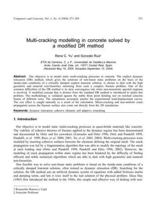
Fig. 1 A notched concrete beam subjected to three point bending
when the solution is far from equilibrium and the estimated frequency is high, the global convergence
rate is remarkably enhanced. The details are going to be shown later on with the examples.
5. Numerical applications
We apply the modified dynamic relaxation method to solve the static crack propagation through a
notched concrete beam subjected to three point bending, see Fig. 1. Particularly, we use the
experiments in Ruiz (1999): three specimens, with depth D = 75, 150 and 300 mm respectively, all
with the same thickness B = 50 mm are modeled. The material parameters for the concrete given in
Table 2 are also taken from Ruiz (1999). The cohesive law adopted in the calculation is the one
suggested in the Model Code (1993) for concrete, Eq. (3).
In previous studies, Camacho and Ortiz (1996) have noted that the accurate description of fracture
processes by means of cohesive elements requires the resolution of the characteristic cohesive length
of the material. Further studies (Ruiz, et al. 2001) showed that in concrete, the element size can be
made to be comparable to the minimum aggregate size, which is 5 mm in our case. So all specimens
are discretized into ten-node quadratic tetrahedral elements and have an element size of 6 mm near
the middle surface. Figs. 2a, b and c show the mesh used in the calculations for the small, medium
and large size specimens, which consists of 2103, 4048 and 10745 10-node quadratic tetrahedrons,
respectively. Concrete bulk is modeled as a finite elastic Neo-Hookean material extended to the
compressible range.
Regarding the tolerances defined in Eq. (21), the product Fext is taken as 1 N for all the
2
ftol simulations, whereas the product K0ketol is taken as 10−8, 10−7 and 5 × 10−7 Nmm for the small,
intermediate and big specimens respectively.
For the purpose of having an order of magnitude in the case of the error norm 1, please remember
that Fext in Eq. (21) represents the modulus of the maximum external force and thus it varies
2
with the scale of the problem. Here we use the experimental values for Fext , which were 800,
2
1300 and 1800 N for the 75, 150 and 300 mm deep beams respectively. Likewise, in the case of the
Table 2 Concrete mechanical properties
fts (MPa) E (GPa) ν Gc (N/m) lch (mm)
3.8 30.5 0.2 62.5 130

Fig. 2 The meshes used in the simulations for D = (a) 75 mm; (b) 150 mm; (c) 300 mm
error norm 2, a convenient choice for K0 in our simulations is the fracture energy expenditure for
each size. This is equivalent to the work of the external forces throughout the whole fracture
process and was measured in the experiments. Its value can be obtained by the product of the
specific fracture energy A 3 and the fracture surface created in each size, which is DB/2. This
multiplication gives 117, 234 and 469 Nmm, the results ordered by size. So, convergence is
achieved in the small beam when the out-of-balance forces are 0.125% of the maximum external
force applied on it and when the total kinetic energy is 8.5 × 10−9% of the total energy consumed by
the fracture process. The corresponding percentages for the intermediate size beam are 0.077 and
4.3 × 10−8 while for the big beam the figures are 0.055 and 1.1 × 10−7.
Before starting to run the model, it is also necessary to set the damping coefficient defining the
verge of an acceptable damping. Our choice for this particular problem, after several trial runs, is
0.3ξmax ( ≈
20ξ 0 in this case), as indicated in Table 1 (command iii. 2). The trial runs showed that
the behavior of the model is not very sensitive to this parameter, i.e., small variations of it lead to
small changes in the convergence rate.
5.1. Comparison between the standard and the modified DR procedures
In this section, we choose one loading step within the simulation of the small specimen to show
the improved convergence rate using the modified DR method. We also check that the modified
method does not affect the final result in any detrimental way by comparing with the results
obtained with the standard DR method. The step chosen corresponds to an imposed displacement of
d = 0.0224 mm. In the previous step there were already four cohesive elements inserted, i.e., the
step corresponds to the initiation of the crack and the system may evolve irreversibly even if there
were no crack advance.
As mentioned in Section 4, when searching for the solution of a particular step, we divide the
iteration process into two phases. During the first phase the specimen is loaded by a small increase
of the imposed displacement and is left to evolve until equilibrium is reached. During this phase we
do not activate the fragmentation algorithm nor do we update the internal variables of the elements
so that no irreversible processes may take place. Actually, as the tetrahedrons are Neo-Hookean, the
only possible irreversibility is concentrated on the fracture development and then, as long as there is
no insertion of new elements nor any updating of the ones that are initially present, overshooting is
avoided altogether. Fig. 3 shows, for both the standard and the modified method, the evolution of
the out-of-balance forces and the kinetic energy of the system during the iterations belonging to this

Fig. 3 Comparison between the standard and modified DR procedures: (a) Out-of-balance forces and (b)
kinetic energy corresponding to the small specimen during the first phase in the step for an imposed
displacement of δ = 0.0224 mm
phase. In fact, the modified procedure is not activated at all during this phase because the forces are
not balanced and Rayleigh’s quotient gives a good estimation of the frequency of vibration of the
beam.
The second phase starts when convergence has been achieved in the first one. Then the program
checks the traction of all the element interfaces and, if the opening criterion is satisfied at any of
them, a cohesive element is inserted there (in this particular case only two new elements are
inserted). Consequently, before moving to the next displacement increment, an iteration loop is
carried out to adjust the solutions because of the stress release coming from the crack propagation.
The elements are updated at convergence of the second phase. Fig. 4 shows the histories of the out-of-
balance forces and of the kinetic energy as the loop proceeds.
Since the dynamic equilibrium has been enhanced by previous iterations during the first phase, the
two methods give the same damping forces and kinetic energy until at some point the program
detects that the system is becoming unbalanced. Moreover, the frequencies generated by the
insertion are considerably bigger than the ones corresponding to the imposed displacements over the
undamaged beam. Thus the modified DR is activated. Fig. 4a shows that the out-of-balance forces
with the modified DR method in practice are of the same order of magnitude as with the standard
procedure. In this particular step they almost reach the value of 6 N (the out-of-balance forces at the
beginning of the first phase were bigger than 400 N, Fig. 3a). The values of the kinetic energy at
the beginning of the phase are relatively high, of the order of 0.01 Nmm according to Fig. 4b,
which is almost three times the maximum energy of the first phase (Fig. 3b). By then the system is
critically damped because the unbalanced forces fall under the tolerance and so the motion is
rapidly stalled. When the system gets unbalanced and, consequently, underdamped, the kinetic
energy starts to oscillate between 0 and 0.001 Nmm (Fig. 4c zooms the energy cycles). Please
remember that the energy needed to split the specimen is 117 Nmm and thus the oscillation is five
orders of magnitude below it. The movement towards the equilibrium position is relatively fast at
this stage and balance is soon restored. Consequently, the damping goes back to its critical value
and final convergence is achieved in a few more iterations as illustrated in Fig. 4d.
In the example shown, where the non-linearity is not strong, it takes 25785 iterations for the

Fig. 4 Comparison between the standard and modified DR procedures: (a) Out-of-balance forces and (b)
kinetic energy corresponding to the small specimen during the second phase in the step for an imposed
displacement of δ = 0.0224 mm. Successive zooms of the kinetic energy curve: (c) noisy response due
to underdamping and (d) final achievement of convergence with critical damping.
standard DR method to converge, whereas the modified DR method only needs 3625. It is not
possible for us to make a comparison in a situation of higher non-linear conditions —for instance a
situation involving many cohesive elements and possible insertions at the same step— simply
because the normal DR method would take too long to arrive at the solution of the static system.
The performance of the precautions taken to avoid overshooting can be evaluated by comparing
the results given by both methods. For this purpose we have rendered the contour plots
corresponding to the stresses along the x axis (σ11) in Figs. 5a and b. Since the stresses are updated
according to the converged solution, the stress distribution given by the standard and by the
modified DR methods look so alike that it is not possible to differentiate between them. In passing
we can notice that the crack does not propagate uniformly across the width of the beam but rather
has a convex front.
We have also rendered the variable called “damage” in Fig. 6. It is defined as the fraction of the
expended fracture energy over the total fracture energy per unit surface. Thus, a damage density of

Fig. 5 Stress σ11 comparison at middle surface for (a) the normal and (b) the modified damping procedures for
the small specimen (D = 75 mm) at an imposed displacement of 0.0224 mm. Dotted contour lines
represent compressive stress values whereas solid contour lines stand for tensile stress values. The
legend is in MPa.
Fig. 6 Cohesive damage comparison at middle surface for (a) the normal and (b) the modified damping
procedures for the small specimen (D = 75 mm) at an imposed displacement of 0.0224 mm.
zero denotes an uncracked surface, whereas a damage density of one is indicative of a fully cracked
or free surface. As it stems from the definition, this variable is proper of cohesive elements only.
Regrettably, our rendering tool reads the values of the variables at the nodes and interpolates them
to get the contour plot (the values are actually computed at the Gauss points and interpolated to the
nodes by the program). This is why in Fig. 6 the damage spreads out of the cohesive elements. In
fact, only the elements where the damage is positive in all the nodes are cohesive: a careful
observation of the figure allows recognition of the six elements present at the end of the step —the
two elements inserted in the step only have a node in the notch tip—, which confirms that the
growth of the crack is not uniform. Regardless, it is not that difficult to observe that Figs. 6a and b

look alike. Again, the numerical differences in the damage incurred using the standard and the
modified methods are very small and cannot be resolved in the contour plot.
All the aforementioned considered, we can conclude that both methodologies lead to the same
results and that overshooting is avoided completely. Likewise, it is pertinent to reiterate here that the
loading steps have to be kept small so that the cohesive elements are inserted gradually. Physically,
this is consistent with a stable crack propagation. Otherwise, it would be the case of an unstable
crack advancement for which neither the standard nor the modified DR method would find a
corresponding static solution. We should have in mind that there may be cases in which static
loading leads to unstable crack propagation, the so called “negative” geometries in Fracture
Mechanics terminology, and again the DR method cannot handle them. In the end, the methodology
that we propose here is close to the actual mechanics of crack propagation, which can be stable but
are never absolutely static.
5.2. Validation against experimental results
5.2.1. Load-displacement curves
The load versus displacement curve for specimens of three different sizes, compared with the
experimental results are shown in Fig. 7.
The model reproduces fairly well the P-δ response of the beams. The calculated maximum load
only differs 0.4% from the experimental one for the small specimen, 3.0% for the intermediate one
and 10.0% for the large specimen, which is specially remarkable if we have in mind that all the
parameters feeding the model are measured experimentally and that we are using a standard
cohesive law. Fig. 7 depicts two horizontal dashed lines to aid the direct visualization of size effect.
The one at the level of 800 N indicates the load peak of the small beam, whereas the one which is
above it marks the load level corresponding to twice such load. The load-peak of the intermediate
Fig. 7 Experimental and numerical load-displacement curves for specimens of three different sizes

beam does not reach that second line in spite that its size doubles the one of the small beam, indeed
it only gets a 70% increase. Likewise, the load-peak given by the big beam is only 30% bigger than
the one of the intermediate (the simulation gives a 50% increase). The experimentally observed size
effect comes naturally from the simulations.
The post-peak behavior is also properly caught by the model. Particularly the simulations for the
small and intermediate specimens give curves that are very close to the ones recorded in the
experiments. The numerical softening branch corresponding to the big beam slightly deviates from
its experimental counterpart, although such a difference can be registered between two identical
actual beams due to the intrinsic concrete heterogeneity.
Nevertheless, the model is not that efficient when it comes to simulate the tail of the P-δ curves.
On the one hand, the degree of fragmentation by the end of the test is very high. On the other hand,
as the specimen is almost split, the displacement increase needed for variations in the loads and
internal variables of the elements is high. Consequently, the number of iterations to achieve
convergence increases dramatically at the end of the test and the run has to be stopped.
5.2.2. Fracture patterns
Three snapshots of the fracture patterns on mid-plane for each one of the simulated specimens are
shown in Fig. 8, where the displacements have been magnified 100 times to aid visualization. Also
shown in the figure are the level contours of damage, as defined above in 5.1. The transition zone
wherein the damage variable takes intermediate values may be regarded as the cohesive zone, and
the crack front may conventionally be identified with the level contour of 1/2. As it is normal in
notched three-point bending tests, the real crack patterns were straight lines starting from the notch
tip and ending in the loading point. Of course, such pattern is easily reproduced by the model.
Indeed, our approach could be readily used in mixed-mode loading cases, which usually generate
more complex fracture patterns than the case we are considering now.
Figs. 8a, d, and g correspond to the peak loads for the small, intermediate and big size beams
respectively. The snapshots in Figs. 8c, f and i catch the moment where the beams are almost
completely broken, while Figs. 8b, e and h represent a point in between which shows how the
fracture zone has developed. For all the sizes it can be noticed that in the peak load the fracture
zone has developed to some degree, but that the crack surfaces are not fully open yet. Later on, the
same zone is more developed while new surfaces are open and the crack front propagates in a non-uniform
way, which can only be observed in a full threedimensional modeling. It is interesting to
note that the crack front is convex in the direction of propagation, a feature which is characteristic
of mode-I crack growth, the exterior of the crack front ostensibly lags behind the interior points. In
Figs. 8c, f and i the crack continues to grow until the specimen is almost completely split and loses
its strength.
6. Conclusions
We have put together a modified explicit dynamic relaxation method in conjunction with the
cohesive theory to solve the static multi-cracking fracture process in a three-point-bend concrete
beam. In calculations, the fracture surface is confined to inter-element boundary elements and,
consequently, the structural cracks predicted by the analysis are necessarily rough. Even though, this

Fig. 8 Snapshots of the fracture patterns at middle surface developed at imposed displacements of (a) 0.05
mm, (b) 0.07 mm and (c) 0.11 mm respectively for the small specimen (D = 75 mm); (d) 0.074 mm,
(e) 0.16 mm and (f) 0.24 mm for the middle size specimen (D = 150 mm); and (g) 0.1 mm, (h) 0.25
mm and (i) 0.50 mm for the large size specimen (D = 300 mm)
numerical roughness in concrete can be made to correspond to the physical roughness by choosing
the element size comparable to the aggregate size, the thus-induced geometrical non-linearity and
the material non-linearity inherent to concrete are hard to handle for traditional static solvers.
The explicit dynamic relaxation method, as an alternative, avoids the use of direct solvers as well
as the large storage requirements associated with large matrices, making it specially attractive in
computational mechanics (Sauvé and Metzger 1995). We have followed the ideas of Underwood
(1983) and Oakley (1995b) for fictitious mass and damping matrices and implemented the explicit
dynamic relaxation method with a concept that is distinct from the standard one. An initial damping
coefficient estimated from the system is adopted to enhance the motion instead of critically damping it

from the beginning. A criterion that measures the balance between reaction forces from the supports
and externally applied forces is used to control the iterations in this stage. While the global kinetic
energy is chosen to control the balance of accuracy and efficiency of the solution for the static system.
Overshooting is avoided by a simple strategy consisting of dividing each step into two distinct
phases. The first one takes the system to the equilibrium point without activating any of the
irreversible mechanisms to reproduce concrete fracture. The second phase starts once equilibrium is
achieved. Then the fragmentation routine inserts as many cohesive elements as necessary and
searches for the new equilibrium point. The stresses, strains, damage limits etc. are only updated at
the end of the iteration process. Of course, the load-displacement increments are taken small
compared to the scale of the problem to avoid a big extent of fragmentation and subsequent fracture
activity at each particular step.
Three sizes of concrete beams with different depth were modeled to validate against the
experimental results of Ruiz (1999). The results show that the model captures the peak load
accurately, the loaddisplacement curve follows closely the experimental results before and after the
peak load. A comparison of the convergence rate between the standard and the modified DR
method reveals the modified concept eliminates the stalling part of the traditional DR method and
makes it a feasible and efficient solution technique for the problem considered.
Acknowledgements
Financial support from the DGICYT, Spain, under grant MAT2003-0843, and from Ministerio de
Fomento, Spain, under grant BOE305/2003. Rena C. Yu thanks the Ministerio de Ciencia y
Tecnología (MCYT), Spain, for the financial support given under the Ramón y Cajal Program.
References
Bazant, Z. P. and Planas, J. (1998), Fracture and Size Effect in Concrete and Other Quasibrittle Materials, CRC
Press, Boca Raton, Florida.
Brew, J. and Brotton, D. M. (1971), “Non-linear structural analysis by dynamic relaxation”, Int. J. Num. Meth.
Eng., 3, 436-483.
Camacho, G. T. and Ortiz, M. (1996), “Computational modelling of impact damage in brittle materials”, Int. J.
Solids Structs., 33(20-22), 2899-2938.
Chen, B. K., Choi, S. K. and Thomson, P. F. (1989), “Analysis of plane strain rolling by the dynamic relaxation
method”, Int. J. Mech. Sci., 31(11/12), 839-851.
Comite Euro-International du Beton (CEB) and the Federation Internationale de la Precont (FIP) (1993), CEB-FIP
Model Code 1990, Thomas Telford Ltd, London, UK.
Cook, R. D., Malkus, D. S. and Plesha, M. E. (1989), Concepts and Applications of Finite Element Analysis,
third edition, John Wiley & Sons, Inc., New York.
Day, A. (1965), “An introduction to dynamic relaxation”, The Engineer, 219, 218-221.
De Andrés, A., P´erez, J. L. and Ortiz, M. (1999), “Elastoplastic finite-element analysis of three-dimensional
fatigue crack growth in aluminum shafts subjected to axial loading”, Int. J. Solids Structs., 36(15), 2231-2258.
Metzger, D. (2003), “Adaptive damping for dynamic relaxation problems with non-monotonic spectral response”,
Int. J. Num. Meth. Eng., 56, 57-80.
Metzger, D. R. and Sauvé, R. G. (1997), “The effect of discretization and boundary conditions on the
convergence rate of the dynamic relaxation method”, Current Topics in the Design and Analysis of Pressure

Vessels and Piping, ASME PVP 354, 105-110.
Oakley, D. R. and Knight, N. F. J. (1995a), “Adaptive dynamic relaxation algorithm for non-linear hyperelastic
structures. Part I. formulation”, Comput. Meth. Appl. Mech. Eng., 126, 67-89.
Oakley, D. R. and Knight, N. F. J. (1995b), “Adaptive dynamic relaxation algorithm for non-linear hyperelastic
structures. part ii. single processor implementation”, Comput. Meth. Appl. Mech. Eng., 126, 91-109.
Oakley, D. R. and Knight, N. F. J. (1995c), “Adaptive dynamic relaxation algorithm for non-linear hyperelastic
structures. part iii. parallel implementation”, Comput. Meth. Appl. Mech. Eng., 126, 111-129.
Oakley, D. R. and Knight, N. F. J. (1996), “Non-linear structural response using adaptive dynamic relaxation on
a massively parallel processor system”, Int. J. Num. Meth. Eng., 39, 235-259.
Ortiz, M. and Pandolfi, A. (1999), “Finite-deformation irreversible cohesive elements for three-dimensional
crack-propagation analysis”, Int. J. Num. Meth. Eng., 44, 1267-1282.
Otter, J. (1965), “Computations for prestressed concrete reactor pressure vessels using dynamic relaxation”, Nucl.
Struct. Eng., 1, 61-75.
Pandolfi, A., Krysl, P. and Ortiz, M. (1999), “Finite element simulation of ring expansion and fragmentation”,
Int. J. Fract., 95, 279-297.
Pandolfi, A. and Ortiz, M. (1998), “Solid modeling aspects of three-dimensional fragmentation”, Eng. Comput,
14(4), 287-308.
Pandolfi, A. and Ortiz, M. (2002), “An efficient adaptive procedure for three-dimensional fragmentation
simulations”, Eng. Comput, 18(2), 148-159.
Papadrakakis, M. (1981), “A method for automated evaluation of the dynamic relaxation parameters”, Comput.
Meth. Appl. Mech. Eng., 25, 35-48.
Pica, A. and Hinton, E. (1980), “Transient and pseudo-transient analysis of mindlin plates”, Int. J. Num. Meth.
Eng., 15, 189-208.
Rericha, P. (1986), “Optimum load time history for non-linear analysis using dynamic relaxation”, Int. J. Num.
Meth. Eng., 23, 2313-2324.
Ruiz, G., Elices, M. and Planas, J. (1999), “Size effect and bond-slip dependence of lightly reinforced concrete
beams”, Minimum Reinforcement in Concrete Beams, ESIS Publications 24, 67-98.
Ruiz, G., Ortiz, M. and Pandolfi, A. (2000), “Three-dimensional finite-element simulation of the dynamic
Brazilian tests on concrete cylinders”, Int. J. Num. Meth. Eng., 48, 963-994.
Ruiz, G., Pandolfi, A. and Ortiz, M. (2001), “Three-dimensional cohesive modeling of dynamic mixed-mode
fracture”, Int. J. Num. Meth. Eng., 52, 97-120.
Sauvé, R. G. and Badie, N. (1993), “Nonlinear shell formulation for reactor fuel channel creep”, Design
Analysis, Robust Methods and Stress Classification, ASME PVP 265, 269-275.
Sauvé, R. G. and Metzger, D. (1995), “Advances in dynamic relaxation techniques for nonlinear finite element
analysis”, Trans. ASME 117, 170-176.
Sauvé, R. G. and Metzger, D. (1996), “A hybrid explicit solution technique for quasi-static transients”, Computer
Technology: Applications and Methodology, ASME PVP 326, 151-157.
Siddiquee, M., Tanaka, T. and Tatsouka, F. (1995), “Tracing the equilibrium path by dynamic relaxation in
materially nonlinear finite element problems”, Int. J. Num. Anal. Meth. Geomech., 19, 749-767.
Thoutireddy, P., Molinari, J. F., Repetto, E. A. and Ortiz, M. (2002), “Tetrahedral composites finite elements”,
Int. J. Num. Meth. Eng., 53, 1337-1351.
Underwood, P. (1983), “Dynamic relaxation”, Comput. Meth. Trans. Anal., 1, 145-265.
Yu, R. C., Pandolfi, A., Coker, D., Ortiz, M. and Rosakis, A. J. (2002), “Three-dimensional modeling of
intersonic shear-crack growth in asymmetrically-loaded unidirectional composite plates”, Int. J. Solids
Structs., 39(25), 6135-6157.
Yu, R. C., Ruiz, G. and Pandolfi, A. (2004), “Numerical investigation on the dynamic behavior of advanced
ceramics”, Eng. Fract. Mech., 71, 897-911.
Zhang, L. G. and Yu, T. X. (1989), “Modified adaptive dynamic relaxation method and its application to elastic-plastic
bending and wrinkling of circular plates”, Comput. Struct., 33(2), 839-851.
CC

J 2004 yu_ruiz_cac

Recommended

Recommended

More Related Content

What's hot

What's hot (20)

Viewers also liked

Viewers also liked (20)

Similar to J 2004 yu_ruiz_cac

Similar to J 2004 yu_ruiz_cac (20)

Recently uploaded

Recently uploaded (20)

J 2004 yu_ruiz_cac