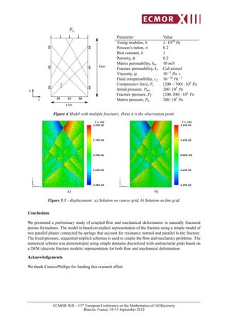
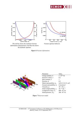
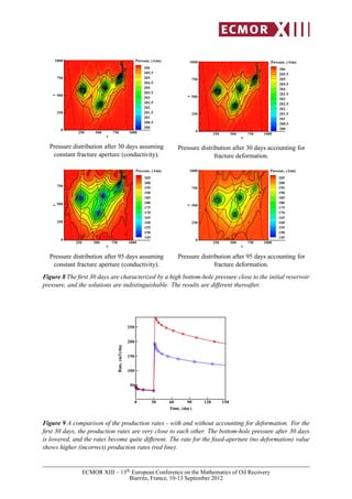
A coupled SPH-DEM model for fluid-structure interaction problems with free-su...
GaripovTT_Ecmor13
1. Introduction
For many reservoirs, the geomechanical effects due to changes in the stress and strain fields can be
quite important. This is especially true for naturally fractured reservoirs. In recent years, there has been
an increased interest in the development of very low-permeability reservoirs, which require stimulation
techniques such as hydraulic fracturing. Successful management such reservoirs requires modeling tools
that account for coupled geomechanics and flow. The importance of geomechanics is not limited to oil
and gas field development. The success of any carbon dioxide sequestration project, or more generally
any underground waste management project, requires detailed understanding of the subsurface geology
and sensitivities to changes in the mechanical equilibrium of the formation.
In this work, we are interested in configurations where the stress field has a significant impact on fluid
flow through changes in the rock and fracture properties. The most common techniques for modeling
flow in naturally fractured media are based on a dual-continuum representation. In these techniques,
the fracture network and the porous matrix are identified as different continua, and their interactions
are modeled using transfer functions. There are many variations of these techniques depending on
the physics of the problem and the simplification strategies. For instance, the original dual-porosity
model by Warren and Root (1963) was developed for highly fractured reservoirs with good fracture
connectivity. Since then, many extensions were proposed to account for more complex physics. In
dual-continuum models, the geometrical distribution of the fractures is lost in the simplification process.
For flow simulation, such approaches are reasonable, as long as, the overall connectivity and the pore-
volume of the fracture network are represented accurately. In contrast, for the mechanical problem, the
geometrical distribution of the fractures has an important impact on the stress and strain fields. Thus,
explicit representation of these features may be necessary.
In recent years, thanks to an increase in computational power, discrete fracture modeling (DFM) tech-
niques have become more popular. In the majority of these models, the fracture network is repre-
sented explicitly using unstructured grids. Different techniques have been proposed to discretize the
flow equations on such grids with special treatment for the fractures. Finite-element based approaches
Kim and Deo (2000), finite-volume based approaches Karimi-Fard et al. (2004)) and control-volume
finite-element approaches Matthäi et al. (2007) are examples. These disctretization techniques are used
either as stand-alone tools to model a limited number of fractures, or as an upscaling tool to construct
coarse reservoir models from detailed fracture characterizations.
Much of the research on the geomechanics of fractured oil reservoirs employs a dual-continuum model
(e.g., Settari (1988), Rutqvist et al. (2002)). Here, we are interested in explicit modeling of the fractured
system for both flow and mechanical deformation. Monteagudo et al. (2011) employed such an ap-
proach, whereby they have developed two separate codes, one for the flow through the fractured porous
medium and one for the mechanical behavior of the porous media. The two codes are coupled by using
an iterative process. Although our objective is to address the same physical problem, our methodology is
different in many aspects including the treatment of the fractures and integration with a general-purpose
research simulator (GPRS).
A fully integrated DFM (discrete fracture model) for flow and geomechanics is presented. The two sets
of equations - flow and mechanics - are discretized using the same unstructured DFM grid. For the flow
equations, we use the finite-volume based DFM approach Karimi-Fard et al. (2004), and for the poro-
elasticity equations, the finite-element approach is considered with special treatment for the fractures.
This mixed formulation leads to a set of coupled nonlinear equations. A fully implicit solution strategy
provides the most stable method but at a high computational cost. However, as shown by Kim (2011),
sequential strategies can provide accurate solution at significantly lower cost. Although these techniques
have been originally developed for porous media without fractures, we explore their applicability for
naturally fractured porous media. A three-dimensional implementation of the methodology is carried
ECMOR XIII – 13th European Conference on the Mathematics of Oil Recovery
Biarritz, France, 10-13 September 2012
2. out within the General Purpose Research Simulator (GPRS) framework developed at Stanford by Cao
(2011) and Jiang (2007) among others.
Mathematical formulation
The quasi-static poro-elasticity model as described by Coussy (2004) is used. The governing equations
are: mass conservation (fluid flow) and momentum balance of the fluid-filled porous skeleton. For
simplicity, only single-phase flow equations are presented here, but the results can be easily extended to
multi-phase flow. The mass conservation equation is written as
(φρf ),t +(ρf vi),i = 0, (1)
where the subscripts t and i indicate derivatives with respect to time and space, respectively.
The Darcy velocity for a single-phase fluid is given by
vi =
k
µf
(−pf,i +ρf gi), (2)
where φ and k are the porosity and permeability; ρf and µf are the fluid density and viscosity; vi and pf
are the fluid velocity and pressure, and gi is the gravity vector.
The poroelasticity equations describing the balance of all forces are defined as follows
σij,j +ρbgi = 0, (3)
where σij is the total stress tensor; ρs is the density of the solid, and ρb = φρf + (1− φ)ρs is the bulk
density. The tensor σij contains the contribution of both the solid skeleton and the pore fluid. Assuming
small deformation and linear elasticity, the constitutive relation for the skeleton are:
σij = Dijklεkl −bpf δij, (4)
where b is the Biot coefficient (Coussy, 2004), and δij is the Kronecker delta. The strain tensor compo-
nents εij are defined as a function of the displacement vector components wi:
εij =
1
2
(wi,j +wj,i). (5)
The stiffness tensor Dijkl is represented as a function of the Lamé rock coefficients µ and λ as follows:
Dijkl = µ δikδjl +δilδjk +λδijδkl. (6)
Eq. 4 describes the balance between inter-grain stresses within the solid matrix and the pressure of the
fluid.
The flow parameters that are sensitive to changes in the stress and strain fields are the porosity and
permeability. The porosity dependence can be expressed as (Nikolaevskiy, 1970; Coussy, 2004):
ECMOR XIII – 13th European Conference on the Mathematics of Oil Recovery
Biarritz, France, 10-13 September 2012
3. φ = φ0 +
(b−φ0)(1−b)
K
(pf − pf0)+b(εv), (7)
where φ0 and pf0 are the reference porosity and pressure, εv = εii is the volumetric strain, and K is the
drainage bulk modulus. Here, the focus is on changes in the fracture permeability due to geomechanical
deformation, and changes in the matrix permeability are assumed to be negligible.
Geomechanical model for fractures
The response of subsurface naturally fractured formations due to changes in the stress and strain fields
can be quite complex. In some cases, the fractured rock is described using an effective medium approach
(Warren and Root, 1963). Another approach is to represent fractures explicitly and use a simple equation
for the fracture permeability, namely, k ∼
a2
f
12
, where af is the fracture aperture. Many experiments have
shown (Ranjith and Viete, 2011) that flow in fractures can be approximated using a cubic relationship
between the pressure gradient and the filtration velocity. A schematic of a ‘natural’ fracture and the
mathematical model used here is shown in Fig. 1. For details regarding this representation, see (Good-
nw -
nw +
n
γτ
γaf
Γf
+
Γf
-
Figure 1 Schematic plot for a natural fracture and a mathematical idealization.
man, 1974; Bandis et al., 1983; Barton and Stephansson, 2011). The ‘springs’ in the model represent
resistances; the parameters γn and γτ represent the resistance in the normal and tangential directions,
respectively. For example, Bandis et al. (1983) suggested the following relationship between the change
in aperture and the normal stress:
σn =
∆af
β1 −β2∆af
, (8)
where β1 and β2 are constants. The aperture, af , is an average value,
af = af0 −∆af
∆af = w+
n −w−
n ,
(9)
where w+
n and w−
n are displacements of the opposite faces and af0 is a maximum aperture when fracture
faces are in contact. We use the Mohr-Coulomb model for shear deformation:
στ = γτσn +c, (10)
where the parameter c represents cohesion. For a fully saturated rock, when the rock grains lose contact,
all the forces are transferred by the fluid, and the total stress is equal to the fluid pressure σn = −pf . This
is possible only when σ
′
n = σn + pf = 0. So, the tensor components σ
′
n are responsible for inter-grain
connections.
Eq. 8 and Eq. 10 connect opposite fracture faces Γ+
f and Γ−
f . To ensure solution continuity, the stress
components must satisfy:
σ
′
ijnj|Γ+
f
= σ
′
ijnj|Γ−
f
(11)
ECMOR XIII – 13th European Conference on the Mathematics of Oil Recovery
Biarritz, France, 10-13 September 2012
4. Numerical treatment
In this paper, a sequential-implicit method is used to solve the coupled flow-mechanics problem. The
solution procedure is shown in Table 1. The Mechanical problem is approximated by finite elements,
while a finite-volume method is used for flow equations. As shown by Kim (2011), the fixed-stress
formulation has good stability and convergence properties. In this procedure, the porosity is calculated
as follows:
φ = φ0 +
(b−φ0)(1−b)
Kdr
(pf − pf0)+
b2
Kdr
(pf − pf0)+
b
Kdr
(σv −σv0 ), (12)
where the volumetric stress is equal to σv = 1
3σii, here σij is the total-stress tensor.
Stage Procedure
0 Initialization:
pt+1,k
f = pt
f , wt+1,k = wt
1a Properties calculation:
volumetric stress σt+1,k
v
porosity φt+1,k
other properties
1b Flow problem:
get pt+1,k+1
f
2 Mechanics problem:
get wt+1,k+1
3 Error norm calculation:
Flow part pt+1,k+1 − pt+1,k
Mechanical part wt+1,k+1 −wt+1,k
IF · < ε then EXIT
4 New sequential step:
pt+1,k
f = pt+1,k+1
f , wt+1,k = wt,k+1
k = k + 1, GOTO stage 1
Table 1 Fixed-stress sequential-implicit procedure
Table 1 shows that the mechanical and flow part are completely independent. This circumstance makes
this method so attractive in code development perspective (Cappa and Rutqvist, 2008; Rutqvist et al.,
2002).
Numerical results
Single fracture model. The proposed model is compared with the example problem presented by Lamb
et al. (2010), which is for single-phase fluid saturating a fractured medium. The medium is 10 by 16
meters with a single fracture inclined at 45 degrees. The model parameters are shown in Fig. 2. The
domain is loaded by an external force Fy = 104Pa on the top as shown in Fig. 2. All boundaries are
closed except the top, which is open to flow. The initial domain pressure is 104Pa. The deformation field
is shown in Fig. 3. Note that the extended finite element method is used by Lamb et al. (2010).
Fractures set model. Fig. 4 shows the schematic for a problem with multiple fractures, and the pa-
ECMOR XIII – 13th European Conference on the Mathematics of Oil Recovery
Biarritz, France, 10-13 September 2012
5. 10m
16m
45
x
y
Fy
undrained boundary
drained boundary
(P = 0 Pa)
P
4
init
= 10 Pa
= 10 Pa
4
Parameter Value
Young modulus, E 40·104 Pa
Poisson’s ratio, ν 0.3
Biot constant, b 1
Porosity, φ 0.1
Matrix permeability, km 10 mD
Fracture permeability, kf 104 mD
Viscosity, µ 10−3 Pa·s
Fluid compressibility, cf 10−10 Pa−1
Compressive force, Fy 104 Pa
Initial pressure, Pinit 104 Pa
Boundary pressure, Ptop 0 Pa
Figure 2 Lamb et al. (2010) single-fracture model.
Figure 3 Reference solution: original solution (left), obtained solution (right).
rameters are given in Fig. 4. The domain is loaded by a constant force, Fy, on the top. The shear
stress components on the fracture are set to zero. All the boundaries are closed. Fig. 5 shows the
x-displacement for different grid sizes. Fig. 6 shows the complex deformation behaviors.
Reservoir model. In the next example, a simple reservoir model is considered (Fig. 7). The matrix
permeability has a log-normal distribution lnN(2.5,0.15). The reservoir is fully saturated with oil.
The model has a set of vertical intersecting fractures and four vertical production wells. A depletion
scenario is considered. The wells, which intersect the fractures, are operated using a constant bottom-
hole pressure. A high bottom-hole pressure, which is close to the initial reservoir pressure, is used
for the first month. Fig. 8 shows that the solutions with and without accounting for deformation are
indistinguishable for the first month. A second period follows, in which the bottom-hole pressure of all
the wells is below 70· 105Pa. The pressure decreases in the fractures faster than in the matrix, and the
fractures start to close. As a result, the fracture conductivities and the production rates decrease.
ECMOR XIII – 13th European Conference on the Mathematics of Oil Recovery
Biarritz, France, 10-13 September 2012
6. 10m
16m
x
y
Fy
A
Parameter Value
Young modulus, E 2·1010 Pa
Poisson’s ration, ν 0.2
Biot constant, b 1
Porosity, φ 0.2
Matrix permeability, km 10 mD
Fracture permeability, kf Calculated
Viscosity, µ 10−3 Pa·s
Fluid compressibility, cf 10−10 Pa−1
Compressive force, Fy (200−700)·105 Pa
Initial pressure, Pinit 200·105 Pa
Fracture pressure, Pf (200,300)·105 Pa
Matrix pressure, Pm 200·105 Pa
Figure 4 Model with multiple fractures. Point A is the observation point.
X
Y
Z
Ux, (m)
3.39E-03
1.70E-03
3.50E-06
-1.69E-03
-3.38E-03
a)
X
Y
Z
Ux, (m)
3.39E-03
1.69E-03
0.00E+00
-1.69E-03
-3.39E-03
b)
Figure 5 X - displacement: a) Solution on course grid, b) Solution on fine grid.
Conclusions
We presented a preliminary study of coupled flow and mechanical deformation in naturally fractured
porous formations. The model is based on explicit representation of the fracture using a simple model of
two parallel planes connected by springs that account for resistance normal and parallel to the fracture.
The fixed-pressure, sequential-implicit schemes is used to couple the flow and mechanics problems. The
numerical scheme was demonstrated using simple domains discretized with unstructured grids based on
a DFM (discrete fracture models) representation for both flow and mechanical deformation.
Acknowledgements
We thank ConocoPhillips for funding this research effort.
ECMOR XIII – 13th European Conference on the Mathematics of Oil Recovery
Biarritz, France, 10-13 September 2012
7. Aperture change, (m)
Hydraulicaperture,(m)
Compressivestress,σn
(Atm)
0 0.0005 0.001 0.0015
0.0005
0.001
0.0015
0.002
0
200
400
600
800
The red line shows the nonlinear fracture
deformation characteristics; the blue line shows
the hydraulic aperture.
Compressive force Fy
, (Atm)Aperture,(m)
300 400 500 600 700
0
0.0005
0.001
0.0015
0.002
Pf = 200 Atm.
Pf = 300 Atm.
Fracture aperture behavior.
Figure 6 Fracture deformation.
x
0
250
500
750
1000
y
250
500
750
1000
Parameter Value
Young modulus, E 2·1010 Pa
Poisson’s ration, ν 0.2
Biot constant, b 1
Porosity, φ 0.2
Matrix permeability, km lnN(2.5,0.15) mD
Fracture permeability, kf Calculated
Viscosity, µ 10−3 Pa·s
Fluid compressibility, cf 10−10 Pa−1
Compressive force, Fy 600·105 Pa
Initial pressure, Pinit 200·105 Pa
Figure 7 Reservoir model.
ECMOR XIII – 13th European Conference on the Mathematics of Oil Recovery
Biarritz, France, 10-13 September 2012
8. x
y
250 500 750 1000
0
250
500
750
1000 Pressure, (Atm)
206
205.5
205
204.5
204
203.5
203
202.5
202
201.5
201
200.5
200
Pressure distribution after 30 days assuming
constant fracture aperture (conductivity).
x
y
250 500 750 1000
0
250
500
750
Pressure, (Atm)
205
200
195
190
185
180
175
170
165
160
155
150
145
Pressure distribution after 95 days assuming
constant fracture aperture (conductivity).
x
y
250 500 750 1000
0
250
500
750
1000 Pressure, (Atm)
206
205.5
205
204.5
204
203.5
203
202.5
202
201.5
201
200.5
200
Pressure distribution after 30 days accounting for
fracture deformation.
x
y
250 500 750 1000
0
250
500
750
1000 Pressure, (Atm)
205
200
195
190
185
180
175
170
165
160
155
150
145
Pressure distribution after 95 days accounting for
fracture deformation.
Figure 8 The first 30 days are characterized by a high bottom-hole pressure close to the initial reservoir
pressure, and the solutions are indistinguishable. The results are different thereafter.
Time, (day)
Rate,(m3)/day
0 30 60 90 120 150
50
100
150
200
250
Figure 9 A comparison of the production rates - with and without accounting for deformation. For the
first 30 days, the production rates are very close to each other. The bottom-hole pressure after 30 days
is lowered, and the rates become quite different. The rate for the fixed-aperture (no deformation) value
shows higher (incorrect) production rates (red line).
ECMOR XIII – 13th European Conference on the Mathematics of Oil Recovery
Biarritz, France, 10-13 September 2012
9. References
Bandis, S., Lumsden, A., Barton, N.:, "Fundamentals of Rock Joint Deformation," Int. J. Rock Mech. Min. and
Geomech. Abstr. (1983), Vol. 20, No. 6
Burton, N. and Stephansson, O.:, "Rock joints," Proceedings of the International Symposium on Rock Joints
(1990), Loen, Norway
Cao, H.:, "Development of Techniques for General Purpose Simulators," Ph.D. thesis (2002), Stanford University
Cappa, F., Rutqvist, J.:, "Modeling of coupled deformation and permeability evolution during fault reactivation
induced by deep underground injection of CO2," International Journal of Greenhouse Gas Control (2011),
Vol. 5
Coussy, O.:, "Poromechanics,", John Wiley and Sons, Ltd (2004)
Goodman, R.:, "The Mechanical Properties of Joints," Proc. 3rd Congr. ISRM (1974), Vol. IA
Jiang, Y. "Techniques for modeling complex reservoirs and advanced wells," Ph.D. thesis (2007), Stanford Uni-
versity
Karimi-Fard, M., Durlofsky, L., Aziz, K.:, "An Efficient Discrete-Fracture Model Applicable for General-Purpose
Reservoir Simulators," SPE (2004), 88812-PA
Kim, J., and Deo, M.:, "Finite Element, Discrete-Fracture Model for Multiphase Flow in Porous Media," AIChE
Journal (2000)
Kim, J., Tchelepi, H., and Juanes, R.:, "Stability, Accuracy, and Efficiency of Sequential Methods for Coupled
Flow and Geomechanics," SPE Journal (2011), 16, No. 2
Lamb, A., Gorman. G., Gosselin O.:, "Finite Element Coupled Deformation and Fluid Flow in Fractured Porous
Media," SPE (2010), 131725
Matthäi, S., Mezentsev, A., and Belayneh, M.:, "Finite Element-Node-Centred Finite-Volume Two-Phase-Flow
Experiments with Fractured Rock Represented by Unstructured Hybrid-Element Meshes," SPE Reservoir Eval-
uation & Engineering (2007)
Monteagudo, J., Rodriguez, A., Florez, H.:, "Simulation of Flow in Discrete Deformable Fractured Porous Media,"
SPE (2011), 141267
Nikolaevskiy, V.:, "Mechanics of Saturated Porous Media," Moscow, "NEDRA" (1970), (in Russian)
Ranjith, P., Viete, D.:, "Applicability of the cubic law for non-Darcian Fracture Flow," Journal of Petroleum
Science and Engineering (2011), No. 78
Rutqvist, J., Wu, Y., Tsang, C., Bodvarsson, G.:, "A Modeling Approach for Analysis of Coupled Multiphase Fluid
Flow, Heat Transfer, and Deformation in Fractured Porous Rock," International Journal of Rock Mechanics and
Mining Sciences (2002), Vol. 39
Settari, A.:, "Numerical Modelling of Hydraulic Fracturing In Underground Rocks," ISRM Conference Paper
(1989), IS-1989-120
Warren, J., Root, P.:, "The Behavior of Naturally Fractured Reservoirs," SPEJ (1963)
ECMOR XIII – 13th European Conference on the Mathematics of Oil Recovery
Biarritz, France, 10-13 September 2012