SlideShare a Scribd company logo
1 of 539
Download to read offline
Table of Chapters
1. Overview of Digital Signal Processing
2. Review of Analog Signal Analysis
3. Discrete-Time Signals and Systems
4. Sampling and Reconstruction of Analog Signals
5. z Transform
6. Discrete-Time Fourier Transform
7. Discrete Fourier Series and Discrete Fourier Transform
8. Responses of Digital Filters
9. Realization of Digital Filters
10. Finite Impulse Response Filter Design
11. Infinite Impulse Response Filter Design
12. Tools and Applications
H. C. So Page 1
Chapter 1: Overview of Digital Signal Processing
Chapter Intended Learning Outcomes:
(i) Understand basic terminology in digital signal processing
(ii) Differentiate digital signal processing and analog signal
processing
(iii) Describe basic digital signal processing application areas
H. C. So Page 2
Signal:
 Anything that conveys information, e.g.,
 Speech
 Electrocardiogram (ECG)
 Radar pulse
 DNA sequence
 Stock price
 Code division multiple access (CDMA) signal
 Image
 Video
H. C. So Page 3
0 0.005 0.01 0.015 0.02
-0.6
-0.4
-0.2
0
0.2
0.4
0.6
0.8
time (s)
vowel
of
"a"
Fig.1.1: Speech
H. C. So Page 4
0 0.5 1 1.5 2 2.5
-50
0
50
100
150
200
250
time (s)
ECG
Fig.1.2: ECG
H. C. So Page 5
0 0.2 0.4 0.6 0.8 1
-1
-0.5
0
0.5
1
time
transmitted
pulse
0 0.2 0.4 0.6 0.8 1
-1
-0.5
0
0.5
1
time
received
pulse
t
Fig.1.3: Transmitted & received radar waveforms
H. C. So Page 6
Radar transceiver sends a 1-D sinusoidal pulse at time 0
It then receives echo reflected by an object at a range of
Reflected signal is noisy and has a time delay of which
corresponds to round trip propagation time of radar pulse
Given the signal propagation speed, denoted by , is
simply related to as:
(1.1)
As a result, the radar pulse contains the object range
information
H. C. So Page 7
 Can be a function of one, two or three independent
variables, e.g., speech is 1-D signal, function of time;
image is 2-D, function of space; wind is 3-D, function of
latitude, longitude and elevation
 3 types of signals that are functions of time:
 Continuous-time (analog) : defined on a continuous
range of time , amplitude can be any value
 Discrete-time : defined only at discrete instants of
time , amplitude can be any value
 Digital (quantized) : both time and amplitude are
discrete, i.e., it is defined only at and
amplitude is confined to a finite set of numbers
H. C. So Page 8
quantized
signal
digital
signal
processor
sample at
analog
signal
sampled
signal
t
amplitude
t
amplitude
0 0
1
t
amplitude
0
1
time and amplitude
continuous
time discrete
amplitude continuous
time and amplitude
discrete
Fig. 1.4: Relationships between , and
H. C. So Page 9
at is close to 2 and
at and
Using 4-bit representation, and , and
in general, the value of is restricted to be an integer
between and according to the two’s complement
representation.
In digital signal processing (DSP), we deal with as it
corresponds to computer-based processing. Throughout the
course, it is assumed that discrete-time signal = digital
signal, or the quantizer has infinite resolution
H. C. So Page 10
System:
 Mathematical model or abstraction of a physical process
that relates input to output, e.g.,
 Grading system: inputs are coursework and examination
marks, output is grade
 Squaring system: input is 5, then the output is 25
 Amplifier: input is )
cos( t
ω , then output is )
cos(
10 t
ω
 Communication system: input to mobile phone is voice,
output from mobile phone is CDMA signal
 Noise reduction system: input is a noisy speech, output
is a noise-reduced speech
 Feature extraction system: input is )
cos( t
ω , output is ω
 Any system that processes digital signals is called a digital
system, digital filter or digital (signal) processor
H. C. So Page 11
Processing:
 Perform a particular function by passing a signal through
system
analog signal
processor
analog
input
analog
output
Fig.1.5: Analog processing of analog signal
analog-to-digital
converter
digital signal
processor
digital-to-analog
converter
analog
input
analog
output
Fig.1.6: Digital processing of analog signal
H. C. So Page 12
Advantages of DSP over Analog Signal Processing
 Allow development with the use of PC, e.g., MATLAB
 Allow flexibility in reconfiguring the DSP operations simply
by changing the program
 Reliable: processing of 0 and 1 is almost immune to noise
and data are easily stored without deterioration
 Lower cost due to advancement of VLSI technology
 Security can be introduced by encrypting/scrambling
 Simple: additions and multiplications are main operations
H. C. So Page 13
DSP Application Areas
 Speech
 Compression (e.g., LPC is a coding standard for
compression of speech data)
 Synthesis (computer production of speech signals, e.g.,
text-to-speech engine by Microsoft)
 Recognition (e.g., automatic telephone number enquiry
system)
 Enhancement (e.g., noise reduction for a noisy speech)
 Audio
 Compression (e.g., MP3 is a coding standard for
compression of audio data)
H. C. So Page 14
 Generation of music by different musical instruments
such as piano, cello, guitar and flute using computer
 Song with low-cost electronic piano keyboard quality
 Automatic music transcription (writing a piece of music
down from a recording)
 Image and Video
 Compression (e.g., JPEG and MPEG is are coding
standards for image and video compression, respectively)
 Recognition such as face, palm and fingerprint
 Enhancement
 Construction of 3-D objects from 2-D images
 Animation, e.g., “Avatar”
H. C. So Page 15
 Communications: encoding and decoding of digital
communication signals
 Astronomy: finding the periods of orbits
 Biomedical Engineering: medical care and diagnosis,
analysis of ECG, electroencephalogram (EEG), nuclear
magnetic resonance (NMR) data
 Bioinformatics: DNA sequence analysis, extracting,
processing, and interpreting the information contained in
genomic and proteomic data
 Finance: market risk management, trading algorithm design,
investment portfolio analysis
H. C. So Page 1
Chapter 2: Review of Analog Signal Analysis
Chapter Intended Learning Outcomes:
(i) Review of Fourier series which is used to analyze
continuous-time periodic signals
(ii) Review of Fourier transform which is used to analyze
continuous-time aperiodic signals
(iii) Review of analog linear time-invariant system
H. C. So Page 2
Fourier series and Fourier transform are the tools for
analyzing analog signals. Basically, they are used for signal
conversion between time and frequency domains:
(2.1)
Fourier Series
 For analysis of continuous-time periodic signals
 Express periodic signals using harmonically related
sinusoids with frequencies where is
called the fundamental frequency
 In the frequency domain, only takes discrete values at
H. C. So Page 3
continuous and periodic discrete and aperiodic
time domain
... ... ... ...
frequency domain
Fig.2.1: Illustration of Fourier series
H. C. So Page 4
A continuous-time function is said to be periodic if there
exists such that
(2.2)
The smallest for which (2.2) holds is called the
fundamental period
The fundamental frequency is related to as:
(2.3)
Every periodic function can be expanded into a Fourier
series as
H. C. So Page 5
(2.4)
where
, (2.5)
are called Fourier series coefficients
is characterized by , the Fourier series coefficients
in fact correspond to the frequency representation of .
Generally, is complex and we use magnitude and phase
for its representation
H. C. So Page 6
(2.6)
and
(2.7)
Example 2.1
Find the Fourier series coefficients for
.
It is clear that the fundamental frequency of is .
According to (2.3), the fundamental period is thus equal to
, which is validated as follows:
H. C. So Page 7
With the use of Euler formulas:
and
we can express as:
By inspection and using (2.4), we have
while all other Fourier series
coefficients are equal to zero
H. C. So Page 8
Example 2.2
Find the Fourier series coefficients for
.
Can we use (2.5)? Why?
With the use of Euler formulas, can be written as:
Using (2.4), we have:
H. C. So Page 9
To plot , we need to compute and for all , e.g.,
and
H. C. So Page 10
Example 2.3
Find the Fourier series coefficients for , which is a
periodic continuous-time signal of fundamental period and
is a pulse with a width of in each period. Over the
specific period from to , is:
with . According to (2.3), the fundamental frequency
is . Using (2.5), we get:
H. C. So Page 11
For :
For :
The reason of separating the cases of and is to
facilitate the computation of , whose value is not
straightforwardly obtained from the general expression
which involves “0/0”. Nevertheless, using ’s rule:
H. C. So Page 12
In summary, if a signal is continuous in time and
periodic, we can write:
(2.4)
The basic steps for finding the Fourier series coefficients are:
1. Determine the fundamental period and fundamental
frequency
2. For all , multiply by , then integrate with
respect to for one period, finally divide the result by .
Usually we separate the calculation into two cases:
and
H. C. So Page 13
Fourier Transform
 For analysis of continuous-time aperiodic signals
 Defined on a continuous range of
The Fourier transform of an aperiodic and continuous-time
signal is:
(2.8)
which is also called spectrum. The inverse transform is
given by
(2.9)
H. C. So Page 14
continuous and aperiodic continuous and aperiodic
time domain frequency domain
Fig.2.2: Illustration of Fourier transform
H. C. So Page 15
The delta function has the following characteristics:
(2.10)
(2.11)
and
(2.12)
where is a continuous-time signal.
(2.10) and (2.11) indicate that has a very large value or
impulse at . That is, is not well defined at
(2.12) is known as the sifting property
H. C. So Page 16
Fig.2.3: Representation of
The unit step function has the form of:
(2.13)
As there is a sudden change from 0 to 1 at , is not
well defined
H. C. So Page 17
Example 2.4
Find the Fourier transform of which is a rectangular
pulse of the form:
Note that the signal is of finite length and corresponds to
one period of the periodic function in Example 2.3. Applying
(2.8) on yields:
H. C. So Page 18
Define the sinc function as:
It is seen that is a scaled sinc function because
Fig.2.4: Fourier transform pair for rectangular pulse of
H. C. So Page 19
Example 2.5
Find the inverse Fourier transform of which is a
rectangular pulse of the form:
Using (2.9), we get:
H. C. So Page 20
Fig.2.5: Fourier transform pair for rectangular pulse of
From Examples 2.4 and 2.5, we observe the duality
property of Fourier transform
Can you guess why we have the duality property?
Example 2.6
Find the Fourier transform of with .
Employing the property of in (2.13) and (2.8), we get:
H. C. So Page 21
Note that when ,
and
Fig.2.6: Magnitude and phase plots for
H. C. So Page 22
Example 2.7
Find the Fourier transform of the delta function .
Using (2.11) and (2.12) with and , we get:
Spectrum of has unit amplitude at all frequencies
Based on , Fourier transform can be used to represent
continuous-time periodic signals. Consider
(2.14)
H. C. So Page 23
Taking the inverse Fourier transform of and employing
Example 2.7, is computed as:
(2.15)
As a result, the Fourier transform pair is:
(2.16)
From (2.4) and (2.16), the Fourier transform pair for a
continuous-time periodic signal is:
(2.17)
H. C. So Page 24
Example 2.8
Find the Fourier transform of which is
called an impulse train.
Clearly, is a periodic signal with a period of . Using
(2.5) and Example 2.7, the Fourier series coefficients are:
with . According to (2.17), the Fourier transform is:
H. C. So Page 25
...
... ...
...
Fig.2.7: Fourier transform pair for impulse train
Fourier transform can be derived from Fourier series:
Consider and :
... ...
Fig.2.8: Constructing from
H. C. So Page 26
is constructed as a periodic version of , with period
According to (2.5), the Fourier series coefficients of are:
(2.18)
where . Noting that for and
for , (2.18) can be expressed as:
(2.19)
H. C. So Page 27
According to (2.8), we can express as:
(2.20)
The Fourier series expansion for is thus:
(2.21)
Considering as or and
as the area of a rectangle whose height is and
width corresponds to the interval of , we obtain
(2.22)
H. C. So Page 28
Linear Time-Invariant (LTI) System
 Linearity: if and are two input-output
pairs, then
 Time-Invariance: if , then
 The input-output relationship for a LTI system is
characterized by convolution:
(2.23)
where , and are input, output and impulse
response, respectively
 Convolution in time domain corresponds to multiplication
in Fourier transform domain, i.e.,
(2.24)
H. C. So Page 29
Proof:
The Fourier transform of is
(2.25)
This suggests that can be computed from inverse
Fourier transform of .
H. C. So Page 1
Chapter 3: Discrete-Time Signals and Systems
Chapter Intended Learning Outcomes:
(i) Understanding deterministic and random discrete-time
signals and ability to generate them
(ii) Ability to recognize the discrete-time system properties,
namely, memorylessness, stability, causality, linearity and
time-invariance
(iii) Understanding discrete-time convolution and ability to
perform its computation
(iv) Understanding the relationship between difference
equations and discrete-time signals and systems
H. C. So Page 2
Discrete-Time Signal
 Discrete-time signal can be generated using a computing
software such as MATLAB
 It can also be obtained from sampling continuous-time
signals in real world
t
Fig.3.1:Discrete-time signal obtained from analog signal
H. C. So Page 3
 The discrete-time signal is equal to only at the
sampling interval of ,
(3.1)
where is called the sampling period
 is a sequence of numbers, , with
being the time index
Basic Sequences
 Unit Sample (or Impulse)
(3.2)
H. C. So Page 4
It is similar to the continuous-time unit impulse which is
defined in (2.10)-(2.12)
is simpler than because it is well defined for all
while is not defined at
 Unit Step
(3.3)
It is similar to to the continuous-time of (2.13)
is well defined for all but is not defined .
H. C. So Page 5
is an important function because it serves as the
building block of any discrete-time signal :
(3.4)
For example, can be expressed in terms of as:
(3.5)
Conversely, we can use to represent :
(3.6)
H. C. So Page 6
Introduction to MATLAB
 MATLAB stands for ”Matrix Laboratory”
 Interactive matrix-based software for numerical and
symbolic computation in scientific and engineering
applications
 Its user interface is relatively simple to use, e.g., we can
use the help command to understand the usage and
syntax of each MATLAB function
 Together with the availability of numerous toolboxes,
there are many useful and powerful commands for various
disciplines
 MathWorks offers MATLAB to C conversion utility
 Similar packages include Maple and Mathematica
H. C. So Page 7
Discrete-Time Signal Generation using MATLAB
A deterministic discrete-time signal satisfies a
generating model with known functional form:
(3.7)
where is a function of parameter vector and time
index . That is, given and , can be produced
e.g., the time-shifted unit sample and unit step
function , where the parameter is
e.g., for an exponential function , we have
where is the decay factor and is the time shift
e.g., for a sinusoid , we have
H. C. So Page 8
Example 3.1
Use MATLAB to generate a discrete-time sinusoid of the
form:
with , , and , which has a duration of
21 samples
We can generate by using the following MATLAB code:
N=21; %number of samples is 21
A=1; %tone amplitude is 1
w=0.3; %frequency is 0.3
p=1; %phase is 1
for n=1:N
x(n)=A*cos(w*(n-1)+p); %time index should be >0
end
Note that x is a vector and its index should be at least 1.
H. C. So Page 9
Alternatively, we can also use:
N=21; %number of samples is 21
A=1; %tone amplitude is 1
w=0.3; %frequency is 0.3
p=1; %phase is 1
n=0:N-1; %define time index vector
x=A.*cos(w.*n+p); %first time index is also 1
Both give
x =
Columns 1 through 7
0.5403 0.2675 -0.0292 -0.3233 -0.5885 -0.8011 -0.9422
Columns 8 through 14
-0.9991 -0.9668 -0.8481 -0.6536 -0.4008 -0.1122 0.1865
Columns 15 through 21
0.4685 0.7087 0.8855 0.9833 0.9932 0.9144 0.7539
Which approach is better? Why?
H. C. So Page 10
To plot , we can either use the commands stem(x) and
plot(x)
If the time index is not specified, the default start time is
Nevertheless, it is easy to include the time index vector in
the plotting command
e.g., Using stem to plot with the correct time index:
n=0:N-1; %n is vector of time index
stem(n,x) %plot x versus n
Similarly, plot(n,x) can be employed to show
The MATLAB programs for this example are provided as
ex3_1.m and ex3_1_2.m
H. C. So Page 11
0 5 10 15 20
-1
-0.8
-0.6
-0.4
-0.2
0
0.2
0.4
0.6
0.8
1
n
x[n]
Fig.3.2: Plot of discrete-time sinusoid using stem
H. C. So Page 12
0 5 10 15 20
-1
-0.8
-0.6
-0.4
-0.2
0
0.2
0.4
0.6
0.8
1
n
x[n]
Fig.3.3: Plot of discrete-time sinusoid using plot
H. C. So Page 13
Apart from deterministic signal, random signal is another
importance signal class. It cannot be described by
mathematical expressions like deterministic signals but is
characterized by its probability density function (PDF).
MATLAB has commands to produce two common random
signals, namely, uniform and Gaussian (normal) variables.
A uniform integer sequence whose values are uniformly
distributed between 0 and , can be generated using:
(3.8)
where and are very large positive integers, is the
reminder of dividing by
Each admissible value of has the same
probability of occurrence of approximately
H. C. So Page 14
We also need an initial integer or seed, say, ,
for starting the generation of
(3.8) can be easily modified by properly scaling and shifting
e.g., a random number which is uniformly between –0.5
and 0.5, denoted by , is obtained from :
(3.9)
The MATLAB command rand is used to generate random
numbers which are uniformly between 0 and 1
e.g., each realization of stem(0:20,rand(1,21)) gives a
distinct and random sequence, with values are bounded
between 0 and 1
H. C. So Page 15
0 5 10 15 20
0
0.5
1
n
0 5 10 15 20
0
0.5
1
n
Fig.3.4: Uniform number realizations using rand
H. C. So Page 16
Example 3.2
Use MATLAB to generate a sequence of 10000 random
numbers uniformly distributed between –0.5 and 0.5 based
on the command rand. Verify its characteristics.
According to (3.9), we use u=rand(1,10000)-0.5 to
generate the sequence
To verify the uniform distribution, we use hist(u,10),
which bins the elements of u into 10 equally-spaced
containers
We see all numbers are bounded between –0.5 and 0.5, and
each bar which corresponds to a range of 0.1, contains
approximately 1000 elements.
H. C. So Page 17
-0.5 0 0.5
0
200
400
600
800
1000
1200
Fig.3.5: Histogram for uniform sequence
H. C. So Page 18
On the other hand, the PDF of u, denoted by , is
such that . The theoretical mean and power of
u, are computed as
and
Average value and power of u in this realization are
computed using mean(u) and mean(u.*u), which give 0.002
and 0.0837, and they align with theoretical calculations
H. C. So Page 19
Gaussian numbers can be generated from the uniform
variables
Given a pair of independent random numbers uniformly
distributed between 0 and 1, , a pair of independent
Gaussian numbers , which have zero mean and unity
power (or variance), can be generated from:
(3.10)
and
(3.11)
The MATLAB command is randn. Equations (3.10) and
(3.11) are known as the Box-Mueller transformation
e.g., each realization of stem(0:20,randn(1,21)) gives a
distinct and random sequence, whose values are fluctuating
around zero
H. C. So Page 20
0 5 10 15 20
-2
0
2
4
n
0 5 10 15 20
-2
-1
0
1
2
n
Fig.3.6: Gaussian number realizations using randn
H. C. So Page 21
Example 3.3
Use the MATLAB command randn to generate a zero-mean
Gaussian sequence of length 10000 and unity power. Verify
its characteristics.
We use w=randn(1,10000) to generate the sequence and
hist(w,50) to show its distribution
The distribution aligns with Gaussian variables which is
indicated by the bell shape
The empirical mean and power of w computed using
mean(w) and mean(w.*w) are and 1.0028
The theoretical standard deviation is 1 and we see that
most of the values are within –3 and 3
H. C. So Page 22
-4 -3 -2 -1 0 1 2 3 4
0
100
200
300
400
500
600
700
Fig.3.7: Histogram for Gaussian sequence
H. C. So Page 23
Discrete-Time Systems
A discrete-time system is an operator which maps an
input sequence into an output sequence :
(3.12)
 Memoryless: at time depends only on at time
Are they memoryless systems?
y[n]=(x[n])2
y[n]=x[n]+ x[n-2]
 Linear: obey principle of superposition, i.e., if
and
then
(3.13)
H. C. So Page 24
Example 3.4
Determine whether the following system with input and
output , is linear or not:
A standard approach to determine the linearity of a system
is given as follows. Let
with
If , then the system is linear. Otherwise,
the system is nonlinear.
H. C. So Page 25
Assigning , we have:
Note that the outputs for and are
and
As a result, the system is linear
H. C. So Page 26
Example 3.5
Determine whether the following system with input and
output , is linear or not:
The system outputs for and are
and . Assigning
, its system output is then:
As a result, the system is nonlinear
H. C. So Page 27
 Time-Invariant: a time-shift of input causes a
corresponding shift in output, i.e., if
then
(3.14)
Example 3.6
Determine whether the following system with input and
output , is time-invariant or not:
A standard approach to determine the time-invariance of a
system is given as follows.
H. C. So Page 28
Let
with
If , then the system is time-invariant.
Otherwise, the system is time-variant.
From the given input-output relationship, is:
Let , its system output is:
As a result, the system is time-invariant.
H. C. So Page 29
Example 3.7
Determine whether the following system with input and
output , is time-invariant or not:
From the given input-output relationship, is of the
form:
Let , its system output is:
As a result, the system is time-variant.
H. C. So Page 30
 Causal: output at time depends on input up to
time
For linear time-invariant (LTI) systems, there is an
alternative definition. A LTI system is causal if its impulse
response satisfies:
(3.15)
Are they causal systems?
y[n]=x[n]+x[n+1]
y[n]=x[n]+x[n-2]
 Stable: a bounded input ( ) produces a
bounded output ( )
H. C. So Page 31
For LTI system, stability also corresponds to
(3.16)
Are they stable systems?
y[n]=x[n]+x[n+1]
y[n]=1/x[n]
Convolution
The input-output relationship for a LTI system is
characterized by convolution:
(3.17)
which is similar to (2.23)
H. C. So Page 32
(3.17) is simpler as it only needs additions and
multiplications
specifies the functionality of the system
 Commutative
(3.18)
and
(3.19)
H. C. So Page 33
Fig.3.8: Commutative property of convolution
H. C. So Page 34
 Linearity
(3.20)
Fig.3.9: Linear property of convolution
H. C. So Page 35
Example 3.8
Compute the output if the input is and the
LTI system impulse response is .
Determine the stability and causality of system.
Using (3.17), we have:
H. C. So Page 36
Alternatively, we can first establish the general relationship
between and with the specific and (3.4):
Substituting yields the same .
Since and for
the system is stable and causal
H. C. So Page 37
Example 3.9
Compute the output if the input is and the
LTI system impulse response is .
Determine the stability and causality of system.
Using (3.17), we have:
H. C. So Page 38
Let and
such that . By employing a change of
variable, is expressed as
Since for , for . For , is:
That is,
H. C. So Page 39
Similarly, is:
Since for , for . For , is:
That is,
H. C. So Page 40
Combining the results, we have:
or
Since , the system is stable.
Moreover, the system is causal because for .
H. C. So Page 41
Example 3.10
Determine where and are
and
Here, the lengths of both and are finite. More
precisely, , , , , , ,
and while all other and have zero
values.
H. C. So Page 42
We still use (3.17) but now it reduces to a finite summation:
By considering the non-zero values of , we obtain:
H. C. So Page 43
Alternatively, for finite-length discrete-time signals, we can
use the MATLAB command conv to compute the convolution
of finite-length sequences:
n=0:3;
x=n.^2+1;
h=n+1;
y=conv(x,h)
The results are
y = 1 4 12 30 43 50 40
As the default starting time indices in both h and x are 1,
we need to determine the appropriate time index for y
H. C. So Page 44
The correct index can be obtained by computing one value
of using (3.17). For simplicity, we may compute :
In general, if the lengths of and are and ,
respectively, the length of is .
H. C. So Page 45
Linear Constant Coefficient Difference Equations
For a LTI system, its input and output are related via
a th-order linear constant coefficient difference equation:
(3.21)
which is useful to check whether a system is both linear and
time-invariant or not
Example 3.11
Determine if the following input-output relationships
correspond to LTI systems:
(a)
(b)
(c)
H. C. So Page 46
We see that (a) corresponds to a LTI system with ,
, and
For (b), we reorganize the equation as:
which agrees with (3.21) when , and
. Hence (b) also corresponds to a LTI system
For (c), it does not correspond to a LTI system because
and are not linear in the equation
Note that if a system cannot be fitted into (3.21), there are
three possibilities: linear and time-variant; nonlinear and
time-invariant; or nonlinear and time-variant
H. C. So Page 47
Example 3.12
Compute the impulse response for a LTI system which is
characterized by the following difference equation:
Expanding (3.17) as
we can easily deduce that only and are nonzero. That
is, the impulse response is:
H. C. So Page 48
The difference equation is also useful to generate the
system output and input.
Assuming that , is computed as:
(3.22)
Assuming that , can be obtained from:
(3.23)
H. C. So Page 49
Example 3.13
Given a LTI system with difference equation of
, compute the system output
for with an input of . It is assumed
that .
The MATLAB code is:
N=50; %data length is N+1
y(1)=1; %compute y[0], only x[n] is nonzero
for n=2:N+1
y(n)=0.5*y(n-1)+2; %compute y[1],y[2],…,y[50]
%x[n]=x[n-1]=1 for n>=1
end
n=[0:N]; %set time axis
stem(n,y);
H. C. So Page 50
0 10 20 30 40 50
0
0.5
1
1.5
2
2.5
3
3.5
4
n
y[n]
system output
Fig.3.10: Output generation with difference equation
H. C. So Page 51
Alternatively, we can use the MATLAB command filter by
rewriting the equation as:
The corresponding MATLAB code is:
x=ones(1,51); %define input
a=[1,-0.5]; %define vector of a_k
b=[1,1]; %define vector of b_k
y=filter(b,a,x); %produce output
stem(0:length(y)-1,y)
The x is the input which has a value of 1 for , while
a and b are vectors which contain and , respectively.
The MATLAB programs for this example are provided as
ex3_13.m and ex3_13_2.m.
H. C. So Page 1
Chapter 4: Sampling and Reconstruction of
Analog Signals
Chapter Intended Learning Outcomes:
(i) Ability to convert an analog signal to a discrete-time
sequence via sampling
(ii) Ability to construct an analog signal from a discrete-time
sequence
(iii) Understanding the conditions when a sampled signal
can uniquely represent its analog counterpart
H. C. So Page 2
Sampling
 Process of converting a continuous-time signal into a
discrete-time sequence
 is obtained by extracting every s where is
known as the sampling period or interval
sample at
analog
signal
discrete-time
signal
Fig.4.1: Conversion of analog signal to discrete-time sequence
 Relationship between and is:
(4.1)
H. C. So Page 3
 Conceptually, conversion of to is achieved by a
continuous-time to discrete-time (CD) converter:
t n
impulse train
to sequence
conversion
CD converter
Fig.4.2: Block diagram of CD converter
H. C. So Page 4
 A fundamental question is whether can uniquely
represent or if we can use to reconstruct
t
Fig.4.3: Different analog signals map to same sequence
H. C. So Page 5
But, the answer is yes when:
(1) is bandlimited such that its Fourier transform
for where is called the bandwidth
(2) Sampling period is sufficiently small
Example 4.1
The continuous-time signal is used as the
input for a CD converter with the sampling period s.
Determine the resultant discrete-time signal .
According to (4.1), is
The frequency in is while that of is
H. C. So Page 6
Frequency Domain Representation of Sampled Signal
In the time domain, is obtained by multiplying by
the impulse train :
(4.2)
with the use of the sifting property of (2.12)
Let the sampling frequency in radian be (or
in Hz). From Example 2.8:
(4.3)
H. C. So Page 7
Using multiplication property of Fourier transform:
(4.4)
where the convolution operation corresponds to continuous-
time signals
Using (4.2)-(4.4) and properties of , is:
H. C. So Page 8
(4.5)
which is the sum of infinite copies of scaled by
H. C. So Page 9
When is chosen sufficiently large such that all copies of
do not overlap, that is, or , we
can get from
...
...
...
...
Fig.4.4: for sufficiently large
H. C. So Page 10
When is not chosen sufficiently large such that ,
copies of overlap, we cannot get from ,
which is referred to aliasing
...
...
...
...
Fig.4.5: when is not large enough
H. C. So Page 11
Nyquist Sampling Theorem (1928)
Let be a bandlimited continuous-time signal with
(4.6)
Then is uniquely determined by its samples ,
, if
(4.7)
The bandwidth is also known as the Nyquist frequency
while is called the Nyquist rate and must exceed it in
order to avoid aliasing
H. C. So Page 12
Application
Biomedical Hz 1 kHz
Telephone speech kHz 8 kHz
Music kHz 44.1 kHz
Ultrasonic kHz 250 kHz
Radar MHz 200 MHz
Table 4.1: Typical bandwidths and sampling frequencies in
signal processing applications
Example 4.2
Determine the Nyquist frequency and Nyquist rate for the
continuous-time signal which has the form of:
The frequencies are 0, and . The Nyquist
frequency is and the Nyquist rate is
H. C. So Page 13
...
...
Fig.4.6: Multiplying and to recover
In frequency domain, we multiply by with
amplitude and bandwidth with , to
obtain , and it corresponds to
H. C. So Page 14
Reconstruction
 Process of transforming back to
sequence to
impulse train
conversion
DC converter
Fig.4.7: Block diagram of DC converter
From Fig.4.6, is
(4.8)
where
H. C. So Page 15
For simplicity, we set as the average of and :
(4.9)
To get , we take inverse Fourier transform of and
use Example 2.5:
(4.10)
where
H. C. So Page 16
Using (2.23)-(2.24), (4.2) and (2.11)-(2.12), is:
(4.11)
which holds for all real values of
H. C. So Page 17
The interpolation formula can be verified at :
(4.12)
It is easy to see that
(4.13)
For , we use ’s rule to obtain:
(4.14)
Substituting (4.13)-(4.14) into (4.12) yields:
(4.15)
which aligns with
H. C. So Page 18
Example 4.3
Given a discrete-time sequence . Generate its
time-delayed version which has the form of
where and is a positive integer. Applying
(4.11) with :
By employing a change of variable of :
Is it practical to get y[n]?
H. C. So Page 19
Note that when , the time-shifted signal is simply
obtained by shifting the sequence by samples:
Sampling and Reconstruction in Digital Signal Processing
CD converter
digital signal
processor
DC converter
Fig.4.8: Ideal digital processing of analog signal
 CD converter produces a sequence from
 is processed in discrete-time domain to give
 DC converter creates from according to (4.11):
(4.16)
H. C. So Page 20
anti-aliasing
filter
digital signal
processor
digital-to-analog
converter
analog-to-digital
converter
Fig.4.9: Practical digital processing of analog signal
 may not be precisely bandlimited ⇒ a lowpass filter or
anti-aliasing filter is needed to process
 Ideal CD converter is approximated by AD converter
 Not practical to generate
 AD converter introduces quantization error
 Ideal DC converter is approximated by DA converter
because ideal reconstruction of (4.16) is impossible
 Not practical to perform infinite summation
 Not practical to have future data
 and are quantized signals
H. C. So Page 21
Example 4.4
Suppose a continuous-time signal is sampled at
a sampling frequency of 1000Hz to produce :
Determine 2 possible positive values of , say, and .
Discuss if or will be obtained when passing
through the DC converter.
According to (4.1) with s:
is easily computed as:
H. C. So Page 22
can be obtained by noting the periodicity of a sinusoid:
As a result, we have:
This is illustrated using the MATLAB code:
O1=250*pi; %first frequency
O2=2250*pi; %second frequency
Ts=1/100000;%successive sample separation is 0.01T
t=0:Ts:0.02;%observation interval
x1=cos(O1.*t); %tone from first frequency
x2=cos(O2.*t); %tone from second frequency
There are 2001 samples in 0.02s and interpolating the
successive points based on plot yields good approximations
H. C. So Page 23
0 5 10 15 20
-1
-0.8
-0.6
-0.4
-0.2
0
0.2
0.4
0.6
0.8
1
n
x[n]
Fig.4.10: Discrete-time sinusoid
H. C. So Page 24
0 0.005 0.01 0.015 0.02
-1
-0.8
-0.6
-0.4
-0.2
0
0.2
0.4
0.6
0.8
1
t
Ω
1
Ω
2
Fig.4.11: Continuous-time sinusoids
H. C. So Page 25
Passing through the DC converter only produces
but not
The Nyquist frequency of is and hence the
sampling frequency without aliasing is
Given Hz or , does not
correspond to
We can recover because the Nyquist frequency
and Nyquist rate for are and
Based on (4.11), is:
with s
H. C. So Page 26
The MATLAB code for reconstructing is:
n=-10:30; %add 20 past and future samples
x=cos(pi.*n./4);
T=1/1000; %sampling interval is 1/1000
for l=1:2000 %observed interval is [0,0.02]
t=(l-1)*T/100;%successive sample separation is 0.01T
h=sinc((t-n.*T)./T);
xr(l)=x*h.'; %approximate interpolation of (4.11)
end
We compute 2000 samples of in s
The value of each at time t is approximated as x*h.'
where the sinc vector is updated for each computation
The MATLAB program is provided as ex4_4.m
H. C. So Page 27
0 0.005 0.01 0.015 0.02
-1
-0.8
-0.6
-0.4
-0.2
0
0.2
0.4
0.6
0.8
1
t
x
r
(t)
Fig.4.12: Reconstructed continuous-time sinusoid
H. C. So Page 28
Example 4.5
Play the sound for a discrete-time tone using MATLAB. The
frequency of the corresponding analog signal is 440 Hz
which corresponds to the A note in the American Standard
pitch. The sampling frequency is 8000 Hz and the signal has
a duration of 0.5 s.
The MATLAB code is
A=sin(2*pi*440*(0:1/8000:0.5));%discrete-time A
sound(A,8000); %DA conversion and play
Note that sampling frequency in Hz is assumed for sound.
The frequencies of notes B, C#, D, E and F# are 493.88 Hz,
554.37 Hz, 587.33 Hz, 659.26 Hz and 739.99 Hz,
respectively. You can easily produce a piece of music with
notes: A, A, E, E, F#, F#, E, E, D, D, C#, C#, B, B, A, A.
H. C. So Page 1
Chapter 5: z Transform
Chapter Intended Learning Outcomes:
(i) Understanding the relationship between transform and
the Fourier transform for discrete-time signals
(ii) Understanding the characteristics and properties of
transform
(iii) Ability to compute transform and inverse transform
(iv) Ability to apply transform for analyzing linear time-
invariant (LTI) systems
H. C. So Page 2
Definition
The transform of , denoted by , is defined as:
(5.1)
where is a continuous complex variable.
Is X(z) real-valued or complex-valued?
Relationship with Fourier Transform
Employing (4.2), we construct the continuous-time sampled
signal with a sampling interval of from :
(5.2)
H. C. So Page 3
Taking Fourier transform of with using properties of :
(5.3)
Defining as the discrete-time frequency parameter
and writing as , (5.3) becomes
(5.4)
which is known as discrete-time Fourier transform (DTFT) or
Fourier transform of discrete-time signals
H. C. So Page 4
is periodic with period :
(5.5)
where is any integer. Since is a continuous complex
variable, we can write
(5.6)
where is magnitude and is angle of .
Employing (5.6), the transform is:
(5.7)
which is equal to the DTFT of . When or ,
(5.7) and (5.4) are identical:
H. C. So Page 5
(5.8)
unit circle
-plane
Fig.5.1: Relationship between and on the -plane
H. C. So Page 6
Region of Convergence (ROC)
ROC indicates when transform of a sequence converges
Generally there exists some such that
(5.9)
where the transform does not converge
The set of values of for which converges or
(5.10)
is called the ROC, which must be specified along with in
order for the transform to be complete
H. C. So Page 7
Assuming that is of infinite length, we decompose :
(5.11)
where
(5.12)
and
(5.13)
Let , is expanded as:
(5.14)
H. C. So Page 8
According to the ratio test, convergence of requires
(5.15)
Let . converges if
(5.16)
That is, the ROC for is .
H. C. So Page 9
Let . converges if
(5.17)
As a result, the ROC for is
Combining the results, the ROC for is :
 ROC is a ring when
 No ROC if and does not exist
H. C. So Page 10
-plane
-plane
-plane
-plane
Fig.5.2: ROCs for , and
Poles and Zeros
Values of for which are the zeros of
Values of for which are the poles of
H. C. So Page 11
In many real-world applications, is represented as a
rational function:
(5.18)
Factorizing and , (5.18) can be written as
(5.19)
How many poles and zeros in (5.18)? What are they?
H. C. So Page 12
Example 5.1
Determine the transform of where is the
unit step function. Then determine the condition when the
DTFT of exists.
Using (5.1) and (3.3), we have
According to (5.10), converges if
Applying the ratio test, the convergence condition is
H. C. So Page 13
Note that we cannot write because may be complex
For , is computed as
Together with the ROC, the transform of is:
It is clear that has a zero at and a pole at .
Using (5.8), we substitute to obtain
As a result, the existence condition for DTFT of is .
H. C. So Page 14
Otherwise, its DTFT does not exist. In general, the DTFT
exists if its ROC includes the unit circle. If
includes , is required.
-plane -plane
-plane
-plane
-plane
-plane
Fig.5.3: ROCs for and when
H. C. So Page 15
Example 5.2
Determine the transform of . Then
determine the condition when the DTFT of exists.
Using (5.1) and (3.3), we have
Similar to Example 5.1, converges if or ,
which aligns with the ROC for in (5.17). This gives
Together with ROC, the transform of is:
H. C. So Page 16
Using (5.8), we substitute to obtain
As a result, the existence condition for DTFT of is .
-plane -plane
-plane
-plane
-plane
-plane
Fig.5.4: ROCs for and when
H. C. So Page 17
Example 5.3
Determine the transform of where
.
Employing the results in Examples 5.1 and 5.2, we have
Note that its ROC agrees with Fig.5.2.
What are the pole(s) and zero(s) of X(z)?
H. C. So Page 18
Example 5.4
Determine the transform of .
Using (5.1) and (3.2), we have
Example 5.5
Determine the transform of which has the form of:
Using (5.1), we have
What are the ROCs in Examples 5.4 and 5.5?
H. C. So Page 19
Finite-Duration and Infinite-Duration Sequences
Finite-duration sequence: values of are nonzero only for
a finite time interval
Otherwise, is called an infinite-duration sequence:
 Right-sided: if for where is an
integer (e.g., with ; with
; with )
 Left-sided: if for where is an
integer (e.g., with )
 Two-sided: neither right-sided nor left-sided (e.g.,
Example 5.3)
H. C. So Page 20
n
Fig.5.5: Finite-duration sequences
H. C. So Page 21
n
Figure 5.6: Infinite-duration sequences
H. C. So Page 22
Sequence Transform ROC
1 All
, ; ,
Table 5.1: transforms for common sequences
H. C. So Page 23
Eight ROC properties are:
P1. There are four possible shapes for ROC, namely, the
entire region except possibly and/or , a ring, or
inside or outside a circle in the -plane centered at the
origin (e.g., Figures 5.5 and 5.6)
P2. The DTFT of a sequence exists if and only if the ROC
of the transform of includes the unit circle (e.g.,
Examples 5.1 and 5.2)
P3: The ROC cannot contain any poles (e.g., Examples 5.1
to 5.5)
P4: When is a finite-duration sequence, the ROC is the
entire -plane except possibly and/or (e.g.,
Examples 5.4 and 5.5)
H. C. So Page 24
P5: When is a right-sided sequence, the ROC is of the
form where is the pole with the largest
magnitude in (e.g., Example 5.1)
P6: When is a left-sided sequence, the ROC is of the
form where is the pole with the smallest
magnitude in (e.g., Example 5.2)
P7: When is a two-sided sequence, the ROC is of the
form where and are two poles with the
successive magnitudes in such that (e.g.,
Example 5.3)
P8: The ROC must be a connected region
Example 5.6
A transform contains three poles, namely, , and
with . Determine all possible ROCs.
H. C. So Page 25
-plane
-plane
-plane
-plane
-plane
-plane -plane
-plane
-plane
-plane
-plane
-plane
Fig.5.7: ROC possibilities for three poles
H. C. So Page 26
What are other possible ROCs?
Inverse z Transform
Inverse transform corresponds to finding given
and its ROC
The transform and inverse transform are one-to-one
mapping provided that the ROC is given:
(5.20)
There are 4 commonly used techniques to evaluate the
inverse transform. They are
1. Inspection
2. Partial Fraction Expansion
3. Power Series Expansion
4. Cauchy Integral Theorem
H. C. So Page 27
Inspection
When we are familiar with certain transform pairs, we can
do the inverse transform by inspection
Example 5.7
Determine the inverse transform of which is
expressed as:
We first rewrite as:
H. C. So Page 28
Making use of the following transform pair in Table 5.1:
and putting , we have:
By inspection, the inverse transform is:
H. C. So Page 29
Partial Fraction Expansion
It is useful when is a rational function in :
(5.21)
For pole and zero determination, it is advantageous to
multiply to both numerator and denominator:
(5.22)
H. C. So Page 30
 When , there are pole(s) at
 When , there are zero(s) at
To obtain the partial fraction expansion from (5.21), the
first step is to determine the nonzero poles,
There are 4 cases to be considered:
Case 1: and all poles are of first order
For first-order poles, all are distinct. is:
(5.23)
For each first-order term of , its inverse
transform can be easily obtained by inspection
H. C. So Page 31
Multiplying both sides by and evaluating for
(5.24)
An illustration for computing with is:
(5.25)
Substituting , we get
In summary, three steps are:
 Find poles
 Find
 Perform inverse transform for the fractions by inspection
H. C. So Page 32
Example 5.8
Find the pole and zero locations of :
Then determine the inverse transform of .
We first multiply to both numerator and denominator
polynomials to obtain:
Apparently, there are two zeros at and . On the
other hand, by solving the quadratic equation at the
denominator polynomial, the poles are determined as
and .
H. C. So Page 33
According to (5.23), we have:
Employing (5.24), is calculated as:
Similarly, is found to be . As a result, the partial
fraction expansion for is
As the ROC is not specified, we investigate all possible
scenarios, namely, , , and .
H. C. So Page 34
For , we notice that
and
where both ROCs agree with . Combining the
results, the inverse transform is:
which is a right-sided sequence and aligns with P5.
For , we make use of
and
H. C. So Page 35
where both ROCs agree with . This implies:
which is a two-sided sequence and aligns with P7.
Finally, for :
and
where both ROCs agree with . As a result, we have:
which is a left-sided sequence and aligns with P6.
H. C. So Page 36
Suppose is the impulse response of a discrete-time LTI
system. Recall (3.15) and (3.16):
and
The three possible impulse responses:
 is the impulse response of a
causal but unstable system
 corresponds to a noncausal
but stable system
 is noncausal and unstable
Which of the h[n] has/have DTFT?
H. C. So Page 37
Case 2: and all poles are of first order
In this case, can be expressed as:
(5.26)
 are obtained by long division of the numerator by the
denominator, with the division process terminating when
the remainder is of lower degree than the denominator
 can be obtained using (5.24).
Example 5.9
Determine which has transform of the form:
H. C. So Page 38
The poles are easily determined as and
According to (5.26) with :
The value of is found by dividing the numerator
polynomial by the denominator polynomial as follows:
That is, . Thus is expressed as
H. C. So Page 39
According to (5.24), and are calculated as
and
With :
and
the inverse transform is:
H. C. So Page 40
Case 3: with multiple-order pole(s)
If has a -order pole at with , this means that
there are repeated poles with the same value of . is:
(5.27)
 When there are two or more multiple-order poles, we
include a component like the second term for each
corresponding pole
 can be computed according to (5.24)
 can be calculated from:
(5.28)
H. C. So Page 41
Example 5.10
Determine the partial fraction expansion for :
It is clear that corresponds to Case 3 with
and one second-order pole at . Hence is:
Employing (5.24), is:
H. C. So Page 42
Applying (5.28), is:
and
H. C. So Page 43
Therefore, the partial fraction expansion for is
Case 4: with multiple-order pole(s)
This is the most general case and the partial fraction
expansion of is
(5.29)
assuming that there is only one multiple-order pole of order
at . It is easily extended to the scenarios when
there are two or more multiple-order poles as in Case 3.
The , and can be calculated as in Cases 1, 2 and 3
H. C. So Page 44
Power Series Expansion
When is expanded as power series according to (5.1):
(5.30)
any particular value of can be determined by finding the
coefficient of the appropriate power of
Example 5.11
Determine which has transform of the form:
Expanding yields
From (5.30), is deduced as:
H. C. So Page 45
Example 5.12
Determine whose transform is given as:
With the use of the power series expansion for :
with can be expressed as
From (5.30), is deduced as:
H. C. So Page 46
Example 5.13
Determine whose transform has the form of:
With the use of
Carrying out long division in with :
From (5.30), is deduced as:
which agrees with Example 5.1 and Table 5.1
H. C. So Page 47
Example 5.14
Determine whose transform has the form of:
We first express as:
Carrying out long division in with :
From (5.30), is deduced as:
which agrees with Example 5.2 and Table 5.1
H. C. So Page 48
Properties of z Transform
1. Linearity
Let and be two transform pairs with
ROCs and , respectively, we have
(5.31)
Its ROC is denoted by , which includes where is
the intersection operator. That is, contains at least the
intersection of and .
Example 5.15
Determine the transform of which is expressed as:
where and . By inspection,
H. C. So Page 49
the transforms of and are:
and
According to the linearity property, the transform of is
Why the ROC is |z|>0.3 instead of |z|>0.2?
2. Time Shifting
A time-shift of in causes a multiplication of in
(5.32)
The ROC for is basically identical to that of
except for the possible addition or deletion of or
H. C. So Page 50
Example 5.16
Find the transform of which has the form of:
Employing the time-shifting property with and:
we easily obtain
Note that using (5.1) with also produces the same
result but this approach is less efficient:
H. C. So Page 51
3. Multiplication by an Exponential Sequence (Modulation)
If we multiply by in the time domain, the variable
will be changed to in the transform domain. That is:
(5.33)
If the ROC for is , the ROC for is
Example 5.17
With the use of the following transform pair:
Find the transform of which has the form of:
H. C. So Page 52
Noting that , can be written as:
By means of the modulation property of (5.33) with the
substitution of and , we obtain:
and
By means of the linearity property, it follows that
which agrees with Table 5.1.
H. C. So Page 53
4. Differentiation
Differentiating with respect to corresponds to
multiplying by in the time domain:
(5.34)
The ROC for is basically identical to that of except
for the possible addition or deletion of or
Example 5.18
Determine the transform of .
Since
and
H. C. So Page 54
By means of the differentiation property, we have
which agrees with Table 5.1.
5. Conjugation
The transform pair for is:
(5.35)
The ROC for is identical to that of
H. C. So Page 55
6. Time Reversal
The transform pair for is:
(5.36)
If the ROC for is , the ROC for is
Example 5.19
Determine the transform of
Using Example 5.18:
and from the time reversal property:
H. C. So Page 56
7. Convolution
Let and be two transform pairs with
ROCs and , respectively. Then we have:
(5.37)
and its ROC includes .
The proof is given as follows.
Let
(5.38)
With the use of the time shifting property, is:
H. C. So Page 57
(5.39)
Transfer Function of Linear Time-Invariant System
A LTI system can be characterized by the transfer function,
which is a transform expression
H. C. So Page 58
Starting with:
(5.40)
Applying transform on (5.40) with the use of the linearity
and time shifting properties, we have
(5.41)
The transfer function, denoted by , is defined as:
(5.42)
H. C. So Page 59
The system impulse response is given by the inverse
transform of with an appropriate ROC, that is,
, such that . This suggests that we
can first take the transforms for and , then multiply
by , and finally perform the inverse transform of
.
Example 5.20
Determine the transfer function for a LTI system whose
input and output are related by:
Applying transform on the difference equation with the use
of the linearity and time shifting properties, is:
H. C. So Page 60
Note that there are two ROC possibilities, namely,
and and we cannot uniquely determine
Example 5.21
Find the difference equation of a LTI system whose transfer
function is given by
Let . Performing cross-multiplication and
inverse transform, we obtain:
Examples 5.20 and 5.21 imply the equivalence between the
difference equation and transfer function
H. C. So Page 61
Example 5.22
Compute the impulse response for a LTI system which is
characterized by the following difference equation:
Applying transform on the difference equation with the use
of the linearity and time shifting properties, is:
There is only one ROC possibility, namely, . Taking the
inverse transform on , we get:
which agrees with Example 3.12
H. C. So Page 62
Example 5.23
Determine the output if the input is and the
LTI system impulse response is
The transforms for and are
and
As a result, we have:
Taking the inverse transform of with the use of the
time shifting property yields:
H. C. So Page 1
Chapter 6: Discrete-Time Fourier Transform (DTFT)
Chapter Intended Learning Outcomes:
(i) Understanding the characteristics and properties of DTFT
(ii) Ability to perform discrete-time signal conversion
between the time and frequency domains using DTFT and
inverse DTFT
H. C. So Page 2
Definition
DTFT is a frequency analysis tool for aperiodic discrete-time
signals
The DTFT of , , has been derived in (5.4):
(6.1)
The derivation is based on taking the Fourier transform of
of (5.2)
As in Fourier transform, is also called spectrum and is
a continuous function of the frequency parameter
H. C. So Page 3
To convert to , we use inverse DTFT:
(6.2)
Proof: Putting (6.1) into (6.2) and using (4.13)-(4.14):
(6.3)
H. C. So Page 4
discrete and aperiodic continuous and periodic
time domain frequency domain
... ...
Fig.6.1: Illustration of DTFT
H. C. So Page 5
is continuous and periodic with a period of
is generally complex, we can illustrate using the
magnitude and phase spectra, i.e., and :
(6.4)
and
(6.5)
where both are continuous in frequency and periodic.
Convergence of DTFT
The DTFT of a sequence converges if
H. C. So Page 6
(6.6)
Recall (5.10) and assume the transform of converges
for region of convergence (ROC) of :
(6.7)
When ROC includes the unit circle:
(6.8)
which leads to the convergence condition for . This
also proves the P2 property of the transform.
H. C. So Page 7
Let be the impulse response of a linear time-invariant
(LTI) system, the following three statements are equivalent:
S1. ROC for the transform of includes unit circle
S2. The system is stable so that
S3. The DTFT of , i.e., , converges
Note that is also known as system frequency response
Example 6.1
Determine the DTFT of .
Using (6.1), the DTFT of is computed as:
H. C. So Page 8
Since
does not exist.
Alternatively, employing the stability condition:
which also indicates that the DTFT does not converge
H. C. So Page 9
Furthermore, the transform of is:
Because does not include the unit circle, there is no
DTFT for .
Example 6.2
Find the DTFT of . Plot the magnitude and
phase spectra for .
Using (6.1), we have
H. C. So Page 10
Alternatively, we can first use transform because
The transform of is evaluated as
As the ROC includes the unit circle, its DTFT exists and the
same result is obtained by the substitution of .
There are two advantages of transform over DTFT:
 transform is a generalization of DTFT and it
encompasses a broader class of signals since DTFT does
not converge for all sequences
 notation convenience of writing instead of .
H. C. So Page 11
To plot the magnitude and phase spectra, we express :
In doing so, and can be written in closed-
forms as:
and
Note that we generally employ (6.4) and (6.5) for
magnitude and phase computation
H. C. So Page 12
In using MATLAB to plot and , we utilize the
command sinc so that there is no need to separately
handle the “0/0” cases due to the sine functions
Recall the definition of sinc function:
As a result, we have:
H. C. So Page 13
The key MATLAB code for is
N=10; %N=10
w=0:0.01*pi:2*pi; %successive frequency point
%separation is 0.01pi
dtft=N.*sinc(w.*N./2./pi)./(sinc(w./2./pi)).*exp(-
j.*w.*(N-1)./2); %define DTFT function
subplot(2,1,1)
Mag=abs(dtft); %compute magnitude
plot(w./pi,Mag); %plot magnitude
subplot(2,1,2)
Pha=angle(dtft); %compute phase
plot(w./pi,Pha); %plot phase
Analogous to Example 4.4, there are 201 uniformly-spaced
points to approximate the continuous functions and
.
H. C. So Page 14
0 0.5 1 1.5 2
0
5
10
Magnitude Response
ω/p
0 0.5 1 1.5 2
-4
-2
0
2
4
Phase Response
ω/p
Fig.6.2: DTFT plots using abs and angle
H. C. So Page 15
Alternatively, we can use the command freqz:
which is ratio of two polynomials in
The corresponding MATLAB code is:
N=10; %N=10
a=[1,-1]; %vector for denominator
b=[1,zeros(1,N-1),-1]; %vector for numerator
freqz(b,a) %plot magnitude & phase (dB)
Note that it is also possible to use and in
this case we have b=ones(N,1) and a=1.
H. C. So Page 16
0 0.2 0.4 0.6 0.8 1
-200
-100
0
100
Normalized Frequency (×π rad/samπle)
Phase
(degrees)
0 0.2 0.4 0.6 0.8 1
-60
-40
-20
0
20
Normalized Frequency (×π rad/samπle)
Magnitude
(dB)
Fig.6.3: DTFT plots using freqz
H. C. So Page 17
The results in Figs. 6.2 and 6.3 are identical, although their
presentations are different:
 at in Fig. 6.2 while that of Fig. 6.3 is 20
dB. It is easy to verify that 10 corresponds to
dB
 units of phase spectra in Figs. 6.2 and 6.3 are radian and
degree, respectively. To make the phase values in both
plots identical, we also need to take care of the phase
ambiguity.
The MATLAB programs for this example are provided as
ex6_2.m and ex6_2_2.m.
H. C. So Page 18
Example 6.3
Find the inverse DTFT of which is a rectangular pulse
within :
where .
Using (6.2), we get:
That is, is an infinite-duration sequence whose values
are drawn from a scaled sinc function.
H. C. So Page 19
Example 6.4
Determine the inverse DTFT of which has the form of:
With the use of , the corresponding transform is
Note that ROC should include the unit circle as DTFT exists
Employing the time shifting property, we get
H. C. So Page 20
Properties of DTFT
Since DTFT is closely related to transform, its properties
follow those of transform. Note that ROC is not involved
because it should include unit circle in order for DTFT exists
1. Linearity
If and are two DTFT pairs, then:
(6.9)
2. Time Shifting
A shift of in causes a multiplication of in :
(6.10)
H. C. So Page 21
3. Multiplication by an Exponential Sequence
Multiplying by in time domain corresponds to a shift
of in the frequency domain:
(6.11)
which agrees with (5.33) by putting and
4. Differentiation
Differentiating with respect to corresponds to
multiplying by :
(6.12)
H. C. So Page 22
Note the RHS is obtained from (5.34) by putting :
(6.13)
5. Conjugation
The DTFT pair for is given as:
(6.14)
6. Time Reversal
The DTFT pair for is given as:
(6.15)
H. C. So Page 23
7. Convolution
If and are two DTFT pairs, then:
(6.16)
In particular, for a LTI system with input , output and
impulse response , we have:
(6.17)
which is analogous to (2.24) for continuous-time LTI
systems
H. C. So Page 24
8. Multiplication
Multiplication in the time domain corresponds to convolution
in the frequency domain:
(6.18)
where denotes convolution within one period
9. Parseval’s Relation
The Parseval’s relation addresses the energy of a sequence:
(6.19)
H. C. So Page 25
With the use of (6.2), the proof is:
(6.20)
H. C. So Page 1
Chapter 7: Discrete Fourier Series & Discrete Fourier
Transform
Chapter Intended Learning Outcomes
(i) Understanding the relationships between the
transform, discrete-time Fourier transform (DTFT), discrete
Fourier series (DFS) and discrete Fourier transform (DFT)
(ii) Understanding the characteristics and properties of DFS
and DFT
(iii) Ability to perform discrete-time signal conversion
between the time and frequency domains using DFS and
DFT and their inverse transforms
H. C. So Page 2
Discrete Fourier Series
DTFT may not be practical for analyzing because
is a function of the continuous frequency variable and we
cannot use a digital computer to calculate a continuum of
functional values
DFS is a frequency analysis tool for periodic infinite-duration
discrete-time signals which is practical because it is discrete
in frequency
The DFS is derived from the Fourier series as follows.
Let be a periodic sequence with fundamental period
where is a positive integer. Analogous to (2.2), we have:
(7.1)
for any integer value of .
H. C. So Page 3
Let be the continuous-time counterpart of . According
to Fourier series expansion, is:
(7.2)
which has frequency components at .
Substituting , and :
(7.3)
Note that (7.3) is valid for discrete-time signals as only the
sample points of are considered.
It is seen that has frequency components at
and the respective complex
exponentials are .
H. C. So Page 4
Nevertheless, there are only distinct frequencies in
due to the periodicity of .
Without loss of generality, we select the following distinct
complex exponentials, , and
thus the infinite summation in (7.3) is reduced to:
(7.4)
Defining , , as the DFS
coefficients, the inverse DFS formula is given as:
(7.5)
H. C. So Page 5
The formula for converting to is derived as follows.
Multiplying both sides of (7.5) by and summing
from to :
(7.6)
Using the orthogonality identity of complex exponentials:
(7.7)
H. C. So Page 6
(7.6) is reduced to
(7.8)
which is also periodic with period .
Let
(7.9)
The DFS analysis and synthesis pair can be written as:
(7.10)
and
(7.11)
H. C. So Page 7
discrete and periodic discrete and periodic
time domain frequency domain
... ...
... ...
Fig.7.1: Illustration of DFS
H. C. So Page 8
Example 7.1
Find the DFS coefficients of the periodic sequence with a
period of . Plot the magnitudes and phases of .
Within one period, has the form of:
Using (7.10), we have
H. C. So Page 9
Similar to Example 6.2, we get:
and
The key MATLAB code for plotting DFS coefficients is
N=5;
x=[1 1 1 0 0];
k=-N:2*N; %plot for 3 periods
Xm=abs(1+2.*cos(2*pi.*k/N));%magnitude computation
Xa=angle(exp(-2*j*pi.*k/5).*(1+2.*cos(2*pi.*k/N)));
%phase computation
The MATLAB program is provided as ex7_1.m.
H. C. So Page 10
-5 0 5 10
0
1
2
3
Magnitude Response
k
-5 0 5 10
-2
-1
0
1
2
Phase Response
k
Fig.7.2: DFS plots
H. C. So Page 11
Relationship with DTFT
Let be a finite-duration sequence which is extracted
from a periodic sequence of period :
(7.12)
Recall (6.1), the DTFT of is:
(7.13)
With the use of (7.12), (7.13) becomes
(7.14)
H. C. So Page 12
Comparing the DFS and DTFT in (7.8) and (7.14), we have:
(7.15)
That is, is equal to sampled at distinct
frequencies between with a uniform frequency
spacing of .
Samples of or DTFT of a finite-duration sequence
can be computed using the DFS of an infinite-duration
periodic sequence , which is a periodic extension of .
H. C. So Page 13
Relationship with z Transform
is also related to transform of according to
(5.8):
(7.16)
Combining (7.15) and (7.16), is related to as:
(7.17)
That is, is equal to evaluated at equally-spaced
points on the unit circle, namely, .
H. C. So Page 14
unit circle
-plane
.
.
.
.
.
.
Fig.7.3: Relationship between , and
H. C. So Page 15
Example 7.2
Determine the DTFT of a finite-duration sequence :
Then compare the results with those in Example 7.1.
Using (6.1), the DTFT of is computed as:
H. C. So Page 16
-2 -1 0 1 2 3 4
0
1
2
3
Magnitude Response
ω/p
-2 -1 0 1 2 3 4
-2
-1
0
1
2
Phase Response
ω/p
Fig.7.4: DTFT plots
H. C. So Page 17
-2 -1 0 1 2 3 4
0
1
2
3
Magnitude Response
ω/p
-2 -1 0 1 2 3 4
-2
0
2
Phase Response
ω/p
Fig.7.5: DFS and DTFT plots with
H. C. So Page 18
Suppose in Example 7.1 is modified as:
Via appending 5 zeros in each period, now we have .
What is the period of the DFS?
What is its relationship with that of Example 7.2?
How about if infinite zeros are appended?
The MATLAB programs are provided as ex7_2.m, ex7_2_2.m
and ex7_2_3.m.
H. C. So Page 19
-2 -1 0 1 2 3 4
0
1
2
3
Magnitude Response
ω/p
-2 -1 0 1 2 3 4
-2
-1
0
1
2
Phase Response
ω/p
Fig.7.6: DFS and DTFT plots with
H. C. So Page 20
Properties of DFS
1. Periodicity
If is a periodic sequence with period , its DFS is
also periodic with period :
(7.18)
where is any integer. The proof is obtained with the use of
(7.10) and as follows:
(7.19)
H. C. So Page 21
2. Linearity
Let and be two DFS pairs with the
same period of . We have:
(7.20)
3. Shift of Sequence
If , then
(7.21)
and
(7.22)
where is the period while and are any integers. Note
that (7.21) follows (6.10) by putting and (7.22)
follows (6.11) via the substitution of .
H. C. So Page 22
4. Duality
If , then
(7.23)
5. Symmetry
If , then
(7.24)
and
(7.25)
Note that (7.24) corresponds to the DTFT conjugation
property in (6.14) while (7.25) is similar to the time
reversal property in (6.15).
H. C. So Page 23
6. Periodic Convolution
Let and be two DFS pairs with the
same period of . We have
(7.26)
Analogous to (6.18), denotes discrete-time convolution
within one period.
With the use of (7.11) and (7.21), the proof is given as
follows:
H. C. So Page 24
(7.27)
To compute where both and are of period ,
we indeed only need the samples with .
H. C. So Page 25
Let . Expanding (7.26), we have:
(7.28)
For :
(7.29)
For :
(7.30)
H. C. So Page 26
A period of can be computed in matrix form as:
(7.31)
Example 7.3
Given two periodic sequences and with period :
and
Compute .
H. C. So Page 27
Using (7.31), is computed as:
The square matrix can be determined using the MATLAB
command toeplitz([1,2,3,4],[1,4,3,2]). That is, we
only need to know its first row and first column.
H. C. So Page 28
Periodic convolution can be utilized to compute convolution
of finite-duration sequences in (3.17) as follows.
Let and be finite-duration sequences with lengths
and , respectively, and which has a length
of
We append and zeros at the ends of and
for constructing periodic and where both are of
period
is then obtained from one period of .
Example 7.4
Compute the convolution of and with the use of
periodic convolution. The lengths of and are 2 and 3
with , , , and .
H. C. So Page 29
The length of is 4. As a result, we append two
zeros and one zero in and , respectively. According to
(7.31), the MATLAB code is:
toeplitz([1,-4,5,0],[1,0,5,-4])*[2;3;0;0]
which gives
2 -5 -2 15
Note that the command conv([2,3],[1,-4,5]) also
produces the same result.
H. C. So Page 30
Discrete Fourier Transform
DFT is used for analyzing discrete-time finite-duration
signals in the frequency domain
Let be a finite-duration sequence of length such that
outside . The DFT pair of is:
(7.32)
and
(7.33)
H. C. So Page 31
If we extend to a periodic sequence with period ,
the DFS pair for is given by (7.10)-(7.11). Comparing
(7.32) and (7.10), for . As a result,
DFT and DFS are equivalent within the interval of
Example 7.5
Find the DFT coefficients of a finite-duration sequence
which has the form of
Using (7.32) and Example 7.1 with , we have:
H. C. So Page 32
Together with whose index is outside the interval of
, we finally have:
If the length of is considered as such that
, then we obtain:
H. C. So Page 33
The MATLAB command for DFT computation is fft. The
MATLAB code to produce magnitudes and phases of is:
N=5;
x=[1 1 1 0 0]; %append 2 zeros
subplot(2,1,1);
stem([0:N-1],abs(fft(x))); %plot magnitude response
title('Magnitude Response');
subplot(2,1,2);
stem([0:N-1],angle(fft(x)));%plot phase response
title('Phase Response');
According to Example 7.2 and the relationship between DFT
and DFS, the DFT will approach the DTFT when we append
infinite zeros at the end of
The MATLAB program is provided as ex7_5.m.
H. C. So Page 34
0 1 2 3 4
0
1
2
3
Magnitude Response
0 1 2 3 4
-2
-1
0
1
2
Phase Response
Fig.7.7: DFT plots with
H. C. So Page 35
Example 7.6
Given a discrete-time finite-duration sinusoid:
Estimate the tone frequency using DFT.
Consider the continuous-time case first. According to
(2.16), Fourier transform pair for a complex tone of
frequency is:
That is, can be found by locating the peak of the Fourier
transform. Moreover, a real-valued tone is:
H. C. So Page 36
From the Fourier transform of , and are located
from the two impulses.
Analogously, there will be two peaks which correspond to
frequencies and in the DFT for .
The MATLAB code is
N=21; %number of samples is 21
A=2; %tone amplitude is 2
w=0.7*pi; %frequency is 0.7*pi
p=1; %phase is 1
n=0:N-1; %define a vector of size N
x=A*cos(w*n+p); %generate tone
X=fft(x); %compute DFT
subplot(2,1,1);
stem(n,abs(X)); %plot magnitude response
subplot(2,1,2);
stem(n,angle(X)); %plot phase response
H. C. So Page 37
0 5 10 15 20
0
5
10
15
20
Magnitude Response
0 5 10 15 20
-2
-1
0
1
2
Phase Response
Fig.7.8: DFT plots for a real tone
H. C. So Page 38
X =
1.0806 1.0674+0.2939i 1.0243+0.6130i
0.9382+0.9931i 0.7756+1.5027i 0.4409+2.3159i
-0.4524+4.1068i -6.7461+15.1792i 6.5451-7.2043i
3.8608-2.1316i 3.3521-0.5718i 3.3521+0.5718i
3.8608+2.1316i 6.5451+7.2043i -6.7461-15.1792i
-0.4524-4.1068i 0.4409-2.3159i 0.7756-1.5027i
0.9382-0.9931i 1.0243-0.6130i 1.0674-0.2939i
Interestingly, we observe that and
. In fact, all real-valued sequences
possess these properties so that we only have to compute
around half of the DFT coefficients.
As the DFT coefficients are complex-valued, we search the
frequency according to the magnitude plot.
H. C. So Page 39
There are two peaks, one at and the other at
which correspond to and , respectively.
From Example 7.2, it is clear that the index refers to
. As a result, an estimate of is:
To improve the accuracy, we append a large number of
zeros to . The MATLAB code for is now modified as:
x=[A*cos(w.*n+p) zeros(1,1980)];
where 1980 zeros are appended.
The MATLAB code is provided as ex7_6.m and ex7_6_2.m.
H. C. So Page 40
0 500 1000 1500 2000
0
5
10
15
20
25
Magnitude Response
0 500 1000 1500 2000
-4
-2
0
2
4
Phase Response
Fig.7.9: DFT plots for a real tone with zero padding
H. C. So Page 41
The peak index is found to be with . Thus
Example 7.7
Find the inverse DFT coefficients for which has a length
of and has the form of
Plot .
Using (7.33) and Example 7.5, we have:
H. C. So Page 42
The main MATLAB code is:
N=5;
X=[1 1 1 0 0];
subplot(2,1,1);
stem([0:N-1],abs(ifft(X)));
subplot(2,1,2);
stem([0:N-1],angle(ifft(X)));
The MATLAB program is provided as ex7_7.m.
H. C. So Page 43
0 1 2 3 4
0
0.2
0.4
Magnitude Response
0 1 2 3 4
-2
-1
0
1
2
Phase Response
Fig.7.10: Inverse DFT plots
H. C. So Page 44
Properties of DFT
Since DFT pair is equal to DFS pair within , their
properties will be identical if we take care of the values of
and when the indices are outside the interval
1. Linearity
Let and be two DFT pairs with the
same duration of . We have:
(7.34)
Note that if and are of different lengths, we can
properly append zero(s) to the shorter sequence to make
them with the same duration.
H. C. So Page 45
2. Circular Shift of Sequence
If , then
(7.35)
Note that in order to make sure that the resultant time
index is within the interval of , we need circular shift,
which is defined as
(7.36)
where the integer is chosen such that
(7.37)
H. C. So Page 46
Example 7.8
Determine where is of length 4
and has the form of:
According to (7.36)-(7.37) with , is determined
as:
H. C. So Page 47
3. Duality
If , then
(7.38)
4. Symmetry
If , then
(7.39)
and
(7.40)
H. C. So Page 48
5. Circular Convolution
Let and be two DFT pairs with the
same duration of . We have
(7.41)
where is the circular convolution operator.
H. C. So Page 49
Fast Fourier Transform
FFT is a fast algorithm for DFT and inverse DFT
computation.
Recall (7.32):
(7.42)
Each involves and complex multiplications and
additions, respectively.
Computing all DFT coefficients requires complex
multiplications and complex additions.
Assuming that , the corresponding computational
requirements for FFT are complex multiplications
and complex additions.
H. C. So Page 50
Direct Computation FFT
Multiplication Addition Multiplication Addition
2 4 2 1 2
8 64 56 12 24
32 1024 922 80 160
64 4096 4022 192 384
1048576 1047552 5120 10240
~ ~ ~ ~
Table 7.1: Complexities of direct DFT computation and FFT
H. C. So Page 51
Basically, FFT makes use of two ideas in its development:
 Decompose the DFT computation of a sequence into
successively smaller DFTs
 Utilize two properties of :
complex conjugate symmetry property:
(7.43)
periodicity in and :
(7.44)
H. C. So Page 52
Decimation-in-Time Algorithm
The basic idea is to compute (7.42) according to
(7.45)
Substituting and for the first and second
summation terms:
(7.46)
H. C. So Page 53
Using since , we have:
(7.47)
where and are the DFTs of the even-index and odd-
index elements of , respectively. That is, can be
constructed from two -point DFTs, namely, and .
Further simplifications can be achieved by writing the
equations as 2 groups of equations as follows:
(7.48)
and
H. C. So Page 54
(7.49)
with the use of and . Equations (7.48) and
(7.49) are known as the butterfly merging equations.
Noting that multiplications are also needed to calculate
, the number of multiplications is reduced from to
.
The decomposition step of (7.48)-(7.49) is repeated times
until 1-point DFT is reached.
H. C. So Page 55
Decimation-in-Frequency Algorithm
The basic idea is to decompose the frequency-domain
sequence into successively smaller subsequences.
Recall (7.42) and employing
and , the even-index DFT coefficients are:
(7.50)
H. C. So Page 56
Using and , the odd-index coefficients are:
(7.51)
and are equal to -point DFTs of
and , respectively. The
decomposition step of (7.50)-(7.51) is repeated times
until 1-point DFT is reached.
H. C. So Page 1
Chapter 8: Responses of Digital Filters
Chapter Intended Learning Outcomes:
(i) Understanding the relationships between impulse
response, frequency response, difference equation and
transfer function in characterizing a LTI system
(ii) Ability to identify infinite impulse response (IIR) and
finite impulse response (FIR) filters. Note that a digital filter
is system which processes discrete-time signals
(iii) Ability to compute system frequency response
H. C. So Page 2
LTI System Characterization
CD converter
discrete-time
LTI system
DC converter
Fig.8.1: Processing of analog signal with LTI filter
The LTI system can be characterized as
 Impulse Response
Let be the impulse response of the LTI filter. Recall from
(3.17), it characterizes the system via the convolution:
(8.1)
is the time-domain response of the LTI filter
H. C. So Page 3
 Frequency Response
We have from (6.17), which is the discrete-time Fourier
transform (DTFT) of (8.1):
(8.2)
is the frequency-domain response of the LTI filter
 Difference Equation
A LTI system satisfies a difference equation of the form:
(8.3)
H. C. So Page 4
 Transfer Function
Taking the transform on both sides of (8.3):
(8.4)
Which of them can uniquely characterize a system?
Which of them cannot?
H. C. So Page 5
Example 8.1
Given the difference equation with input and output :
Find all possible ways to compute given .
In fact, there are two ways to compute .
A straightforward and practical way is to implement a causal
system by using the difference equation recursively with a
given initial condition of :
H. C. So Page 6
On the other hand, it is possible to implement a noncausal
system via reorganizing the difference equation as:
In doing so, we need an initial future value of and
future inputs, and the recursive implementation is:
As a result, generally the difference equation cannot
uniquely characterize the system.
H. C. So Page 7
Nevertheless, if causality is assumed, then the difference
equation corresponds to a unique LTI system.
Alternatively, we can also study the computation of
using system transfer function :
Since the ROC is not specified, there are two possible cases,
namely, and .
For or , using inverse transform:
H. C. So Page 8
which corresponds to a causal system.
The same result can also be produced by first finding the
system impulse response via inverse transform of
:
and then computing .
H. C. So Page 9
For or , using inverse transform:
which corresponds to a noncausal system.
Example 8.2
Discuss all possibilities for the LTI system whose input
and output are related by:
H. C. So Page 10
Taking transform on the difference equation yields:
There are 3 possible choices:
: The ROC is outside the circle with radius
characterized by the largest-magnitude pole. The system
can be causal but is not stable since the ROC does not
include the unit circle
: The system is stable because the ROC includes
the unit circle but not causal
: The system is unstable and noncausal
H. C. So Page 11
Impulse Response of Digital Filters
When is a rational function of with only first-order
poles, we have from (5.26):
(8.5)
where the first component is present only if .
If the system is causal, then the ROC must be of the form
where is the largest-magnitude pole.
H. C. So Page 12
According to this ROC, the impulse response is:
(8.6)
There are two possible cases for (8.6) which correspond to
IIR and FIR filters:
 IIR Filter
If or there is at least one pole, the system is referred
to as an IIR filter because is of infinite duration.
 FIR Filter
If or there is no pole, the system is referred to as a
FIR filter because is of finite duration.
H. C. So Page 13
Notice that the definitions of IIR and FIR systems also hold
for noncausal systems.
Example 8.3
Determine if the following difference equations correspond
to IIR or FIR systems. All systems are assumed causal.
(a)
(b)
Taking the transform on (a) yields
which has one pole. For causal system:
H. C. So Page 14
which is a right-sided sequence and corresponds to an IIR
system as is of infinite duration.
Similarly, we have for (b):
which does not have any nonzero pole. Hence
which corresponds to a FIR system as is of finite
duration.
H. C. So Page 15
Frequency Response of Digital Filters
The frequency response of a LTI system whose impulse
response is obtained by taking the DTFT of :
(8.7)
According to (5.8), is also obtained if is available:
(8.8)
assuming that the ROC of includes the unit circle.
H. C. So Page 16
Example 8.4
Plot the frequency response of the system with impulse
response of the form:
where
Following Example 7.6, we append a large number of zeros
at the end of prior to performing discrete Fourier
transform (DFT) to produce more DTFT samples.
Is it a low-pass filter? Why?
The MATLAB program is provided as ex8_4.m.
H. C. So Page 17
0 0.5 1 1.5 2
0
5
10
Magnitude Response
ω/p
0 0.5 1 1.5 2
-4
-2
0
2
4
Phase Response
ω/p
Fig.8.2: Frequency response for sinc
H. C. So Page 18
Example 8.5
Plot the frequency response of the system with transfer
function of the form:
It is assumed that the ROC of includes the unit circle.
The MATLAB code is
b=[1,2,3];
a=[2,3,4];
freqz(b,a);
Is it a lowpass filter? Why?
The MATLAB program is provided as ex8_5.m.
H. C. So Page 19
0 0.2 0.4 0.6 0.8 1
-20
-10
0
10
20
Normalized Frequency (×π rad/samπle)
Phase
(degrees)
0 0.2 0.4 0.6 0.8 1
-4
-3
-2
-1
0
Normalized Frequency (×π rad/samπle)
Magnitude
(dB)
Fig.8.3: Frequency response for second-order system
H. C. So Page 1
Chapter 9: Realization of Digital Filters
Chapter Intended Learning Outcomes:
(i) Ability to implement finite impulse response (FIR) and
infinite impulse response (IIR) filters using different
structures in terms of block diagram and signal flow graph
(ii) Ability to determine the system transfer function and
difference equation given the corresponding block diagram
or signal flow graph representation.
H. C. So Page 2
Filter Implementation
When causality is assumed, a LTI filter can be uniquely
characterized by its transfer function :
(9.1)
or the corresponding difference equation:
(9.2)
where and are the system input and output
H. C. So Page 3
Assuming , the output is:
(9.3)
Assigning and yields
(9.4)
Computing involves and
. That is, we need
 Delay elements or storage
 Multipliers
 Adders (subtraction is considered as addition)
H. C. So Page 4
How many storage elements are needed?
How many multipliers are needed?
How many adders are needed?
Computations of ]
[n
y can be arranged in different ways to
give the same difference equation, which leads to different
structures for realization of discrete-time LTI systems
4 basic forms of implementations, namely, direct form,
canonic form, cascade form and parallel form will be
described
An implementation can be represented using either a block
diagram or a signal flow graph
H. C. So Page 5
Block Diagram Representation
adder
multiplier
unit delay
Fig.9.1: Basic operations in block diagram
H. C. So Page 6
Although an adder can generally deal with more than two
sequences, here we consider two signals in order to align
with practical implementation in microprocessors.
When , it corresponds to signal amplification while the
signal is attenuated for . Note that a multiplier usually
has the highest implementation or computational cost and
thus it is desired to reduce the number of multipliers in
different systems, if possible.
The transfer function corresponds to a unit delay. It can
be implemented by providing a storage register for each
unit delay in digital implementation. If the required number
of samples of delay is , then the corresponding system
function is .
H. C. So Page 7
Signal Flow Graph Representation
adder
multiplier
unit delay
Figure 9.2: Basic operations in signal flow graph
H. C. So Page 8
Its basic elements are branches with directions, and nodes.
That is, a signal flow graph is a set of directed branches
that connect at nodes.
Signal at a node of a flow graph is equal to the sum of the
signals from all branches connecting to the node.
Signal out of a branch is equal to the branch gain times the
signal into the branch.
Branch gain can refer to a scalar or a transfer function of
corresponding to multiplication or unit delay operation,
respectively.
When the branch gain is unity, it is left unlabeled.
A signal flow graph provides an alternative but equivalent
graphical representation to a block diagram structure
H. C. So Page 9
Example 9.1
Draw the block diagram and signal flow graph
representations of a LTI system whose input and output
satisfy the following difference equation:
Fig.9.3: Illustration of block diagram
H. C. So Page 10
Fig.9.4: Illustration of signal flow graph
2 adders, 3 multipliers and 2 delay elements are required to
implement the system.
H. C. So Page 11
Structures for FIR Filter
For FIR filter, its transfer function does not contain pole.
That is, setting and in (9.1) yields
a FIR system:
(9.5)
while the corresponding difference equation is:
(9.6)
H. C. So Page 12
1. Direct Form
Comparing (9.6) with the convolution formula of (3.18),
correspond to the system impulse response :
(9.7)
(9.6) can also be written as:
(9.8)
The direct form follows straightforwardly from the difference
equation.
H. C. So Page 13
The implementation needs memory locations for storing
previous inputs of , multiplications and
additions for computing each output value of .
Fig.9.5: Direct form of FIR filter
H. C. So Page 14
2. Cascade Form
Expressing (9.5) as products of second-order polynomial
system functions via factorization:
(9.9)
where is the largest integer contained in
. Note that when is odd, one of the will be
zero. Assuming that is even, this implementation needs
storage elements, multiplications and additions,
for computing each output value of .
Why second-order polynomial instead of first-order
polynomial?
H. C. So Page 15
Fig.9.6: Cascade form of FIR filter
(9.10)
and
(9.11)
H. C. So Page 16
Taking transform on (9.10) and (9.11):
(9.12)
and
(9.13)
Substituting (9.13) into (9.12) yields:
(9.14)
Extending (9.14) to , we finally get:
(9.15)
H. C. So Page 17
To save the computational complexity, we express (9.9) as:
(9.16)
where , and ,
. That is, all are normalized to 1.
Assuming that is even, (9.16) needs delay elements,
multiplications and additions, for computing each
output value of
H. C. So Page 18
Fig.9.7: Cascade form of FIR filter with smaller complexity
Example 9.2
Draw the signal flow graph using the cascade form for the
LTI system whose transfer function is:
H. C. So Page 19
To factorize , we use the MATLAB command roots([1 1
1 1 1]) to solve for the roots:
0.3090 + 0.9511i
0.3090 - 0.9511i
-0.8090 + 0.5878i
-0.8090 - 0.5878i
Hence can be factorized as
Although it can be realized with first-order sections,
complex coefficients are needed, which implies higher
computational cost. To guarantee real-valued coefficients,
we group the sections of complex conjugates together:
H. C. So Page 20
Fig.9.8: Two possible cascade forms for FIR filter
H. C. So Page 21
Structures for IIR Filter
When there is at least one pole in , it corresponds to an
IIR filter. The corresponding transfer function is thus:
(9.17)
That is, IIR filter is the general form of any discrete-time
LTI system.
H. C. So Page 22
1. Direct Form
It realizes (9.4) in an explicit manner via decomposing it
into a pair of difference equations:
(9.18)
and
(9.19)
The direct form can also be obtained by decomposing
into two transfer functions as:
(9.20)
where
H. C. So Page 23
(9.21)
and
(9.22)
In the transform domain, we have:
(9.23)
and
(9.24)
H. C. So Page 24
Fig.9.9: Direct form of IIR filter
H. C. So Page 25
The direct form implementation needs memory
locations, multiplications and additions,
for computing each output value of .
2. Canonic Form
On the other hand, we can first pass through the filter
to produce an intermediate signal . The is then
passed through the system to give :
(9.25)
and
(9.26)
H. C. So Page 26
Applying inverse transform, we get:
(9.27)
and
(9.28)
which can be considered as an alternative direct form.
H. C. So Page 27
Fig.9.10: Alternative direct form of IIR filter
H. C. So Page 28
Assume . Since the same signals
, are stored in the two chains of
storage elements, they can be combined to reduce the
memory requirement.
In general, the minimum number of delay elements
required is .
It is called canonic form because this implementation
involves the minimum number of storages.
H. C. So Page 29
Fig.9.11: Canonic form of IIR filter
H. C. So Page 30
Example 9.3
Draw the block diagrams using the direct and canonic forms
for the LTI system whose transfer function is:
According to (9.18)-(9.19):
Based on (9.27)-(9.28):
H. C. So Page 31
Fig.9.12: Direct form of second-order IIR filter
Fig.9.13: Canonic form of second-order IIR filter
H. C. So Page 32
3. Cascade Form
We factorize the numerator and denominator polynomials in
terms of second-order polynomial system functions as:
(9.29)
Without loss of generality, it is assumed that so that
. Note that when or is odd, one of the
or will be zero.
H. C. So Page 33
Each second-order subsystem
(9.30)
can be realized in either the direct or canonic form.
Nevertheless, the canonic form is preferred because it
requires the minimum number of delay elements.
In IIR filter implementation, we can group the numerator
and denominator of (9.30) in different ways, leading to
different pole and zero combinations in each of the second-
order sections.
For example, there are four possible cascade realizations for
a fourth-order IIR filter with .
H. C. So Page 34
H. C. So Page 35
Fig.9.14: 4 possible cascade realizations for 4th-order IIR filter
H. C. So Page 36
To save the computational complexity, we express (9.29) as
(9.31)
where , and ,
.
Assuming that is even with , the cascade
implementation of (9.31) needs or delay elements,
multiplications and additions, for computing
each . That is, its memory and computational
requirements are equal to those of the direct form.
H. C. So Page 37
Example 9.4
Draw the signal flow graph using the cascade form with
first-order sections for the LTI system whose transfer
function is:
For each first-order section, canonic form is assumed.
Solving the quadratic equations of the numerator and
denominator polynomials, we can factorize as:
There are four possible cascade forms for :
H. C. So Page 38
Note that although all four realizations are equivalent for
infinite precision, they may differ in actual implementation
when finite-precision numbers are employed.
H. C. So Page 39
Fig.9.15: 4 possible cascade realizations with 1st-order sections
H. C. So Page 40
Example 9.5
Consider a LTI system whose transfer function is:
Find the number of possible combinations of cascade form
with second-order sections. Determine if the system is
stable or not.
Further factorizing yields:
H. C. So Page 41
For the numerator polynomials, there are 3 grouping
possibilities in terms of second-order sections as follows:
There are also 3 grouping possibilities for the denominator:
H. C. So Page 42
Each fourth-order IIR filter can be realized in four possible
cascade forms.
As a result, the number of possible cascade form
combinations with second-order sections for is
.
When implementing a filter, causality is always assumed
because it is impossible to realize a noncausal system
where the output depends on future input. It is clear that
the region of convergence (ROC) for causal is .
Since the ROC does not include the unit circle, the system is
not stable.
In summary, a causal system is stable when all poles are
inside the unit circle.
H. C. So Page 43
4. Parallel Form
The idea of the parallel form is similar to the partial fraction
expansion of transform:
(9.32)
where . But now we use second-order
sections in order to ensure all , , and are
real.
Note that when , the first summation term in (9.32)
will not be included.
H. C. So Page 44
Example 9.6
Draw the block diagram using parallel form for a LTI system
whose transfer function is:
Following the long division as in Example 5.9, we obtain:
H. C. So Page 45
Fig.9.16: Parallel form with second-order section
As the poles of are real, we can also express in
terms of first-order sections as:
H. C. So Page 46
Fig.9.17: Parallel form with first-order sections
H. C. So Page 47
Example 9.7
Determine the transfer function and the difference
equation which relates and for
Fig.9.18: LTI system parameterized by and
H. C. So Page 48
We first introduce an intermediate sequence to relate
and . Then we can establish:
and
Applying transform yields:
and
From the second equation, we have:
H. C. So Page 49
Substituting it into the first equation, we finally have:
Taking the inverse transform gives:
H. C. So Page 50
Comparison of Different Structures
The major factors that affect our choice of a specific
realization are computational complexity, memory
requirement, and finite word-length effects. Assuming that
is even with :
Structure Multiplication Addition Register
Direct form
Cascade form
Table 9.1: FIR filter structure comparison
Structure Multiplication Addition Register
Direct form
Canonic form
Cascade form
Parallel form
Table 9.2: IIR filter structure comparison
H. C. So Page 51
Computations of the direct form can be reduced if the FIR
filter coefficients are symmetric or anti-symmetric.
When the filter coefficients are expressed using infinite
precision numbers, all realizations are same. However, in
practice, they are processed in registers which have finite
word-lengths. In the presence of quantization errors, the
cascade and parallel realizations are more robust than the
direct and canonic forms, that is, they have frequency
responses closer to the desired responses.
FIR filters are less sensitive than IIR filters to finite word-
length effects.
For a feasible system, it should be causal and stable.
In cascade and parallel realizations of IIR filters, system
stability can be easily monitored by checking pole locations.
H. C. So Page 1
Chapter 10: FIR Filter Design
Chapter Intended Learning Outcomes:
(i) Understanding of the characteristics of linear-phase finite
impulse response (FIR) filters
(ii) Ability to design linear-phase FIR filters according to
predefined specifications using the window and frequency
sampling methods
H. C. So Page 2
Steps in Digital Filter Design
1. Specification Determination
The first step is to obtain the filter specifications or
requirements which are determined by the applications.
Suppose the requirement is a lowpass filter with cutoff
frequency of to achieve a task of noise reduction
The filter specification can be described by discrete-time
Fourier transform (DTFT) :
(10.1)
which specifies both the magnitude and phase
H. C. So Page 3
Fig.10.1: Ideal lowpass filter
 unity gain for the whole range of
 complete suppression for
 step change in frequency response at
H. C. So Page 4
passband transition stopband
Fig.10.2: Practical
 passband corresponds to where is the
passband frequency and is the passband ripple or
tolerance which is the maximum allowable deviation from
unity in this band
DSP 2.pdf
DSP 2.pdf
DSP 2.pdf
DSP 2.pdf
DSP 2.pdf
DSP 2.pdf
DSP 2.pdf
DSP 2.pdf
DSP 2.pdf
DSP 2.pdf
DSP 2.pdf
DSP 2.pdf
DSP 2.pdf
DSP 2.pdf
DSP 2.pdf
DSP 2.pdf
DSP 2.pdf
DSP 2.pdf
DSP 2.pdf
DSP 2.pdf
DSP 2.pdf
DSP 2.pdf
DSP 2.pdf
DSP 2.pdf
DSP 2.pdf
DSP 2.pdf
DSP 2.pdf
DSP 2.pdf
DSP 2.pdf
DSP 2.pdf
DSP 2.pdf
DSP 2.pdf
DSP 2.pdf
DSP 2.pdf
DSP 2.pdf
DSP 2.pdf
DSP 2.pdf
DSP 2.pdf
DSP 2.pdf
DSP 2.pdf
DSP 2.pdf
DSP 2.pdf
DSP 2.pdf
DSP 2.pdf
DSP 2.pdf
DSP 2.pdf
DSP 2.pdf
DSP 2.pdf
DSP 2.pdf
DSP 2.pdf
DSP 2.pdf
DSP 2.pdf
DSP 2.pdf
DSP 2.pdf
DSP 2.pdf
DSP 2.pdf
DSP 2.pdf
DSP 2.pdf
DSP 2.pdf
DSP 2.pdf
DSP 2.pdf
DSP 2.pdf
DSP 2.pdf
DSP 2.pdf
DSP 2.pdf
DSP 2.pdf
DSP 2.pdf
DSP 2.pdf
DSP 2.pdf
DSP 2.pdf
DSP 2.pdf
DSP 2.pdf
DSP 2.pdf
DSP 2.pdf
DSP 2.pdf
DSP 2.pdf
DSP 2.pdf
DSP 2.pdf
DSP 2.pdf
DSP 2.pdf
DSP 2.pdf
DSP 2.pdf
DSP 2.pdf
DSP 2.pdf
DSP 2.pdf
DSP 2.pdf
DSP 2.pdf
DSP 2.pdf
DSP 2.pdf
DSP 2.pdf
DSP 2.pdf
DSP 2.pdf
DSP 2.pdf
DSP 2.pdf
DSP 2.pdf
DSP 2.pdf
DSP 2.pdf
DSP 2.pdf
DSP 2.pdf
DSP 2.pdf
DSP 2.pdf
DSP 2.pdf
DSP 2.pdf
DSP 2.pdf
DSP 2.pdf
DSP 2.pdf
DSP 2.pdf
DSP 2.pdf
DSP 2.pdf
DSP 2.pdf
DSP 2.pdf
DSP 2.pdf
DSP 2.pdf
DSP 2.pdf
DSP 2.pdf
DSP 2.pdf
DSP 2.pdf
DSP 2.pdf
DSP 2.pdf
DSP 2.pdf
DSP 2.pdf
DSP 2.pdf
DSP 2.pdf
DSP 2.pdf
DSP 2.pdf
DSP 2.pdf
DSP 2.pdf
DSP 2.pdf
DSP 2.pdf
DSP 2.pdf
DSP 2.pdf
DSP 2.pdf
DSP 2.pdf
DSP 2.pdf
DSP 2.pdf
DSP 2.pdf
DSP 2.pdf
DSP 2.pdf
DSP 2.pdf
DSP 2.pdf
DSP 2.pdf
DSP 2.pdf
DSP 2.pdf
DSP 2.pdf
DSP 2.pdf
DSP 2.pdf
DSP 2.pdf
DSP 2.pdf
DSP 2.pdf
DSP 2.pdf
DSP 2.pdf
DSP 2.pdf
DSP 2.pdf
DSP 2.pdf
DSP 2.pdf
DSP 2.pdf
DSP 2.pdf
DSP 2.pdf
DSP 2.pdf
DSP 2.pdf
DSP 2.pdf
DSP 2.pdf
DSP 2.pdf
DSP 2.pdf
DSP 2.pdf
DSP 2.pdf
DSP 2.pdf
DSP 2.pdf
DSP 2.pdf
DSP 2.pdf
DSP 2.pdf
DSP 2.pdf
DSP 2.pdf
DSP 2.pdf
DSP 2.pdf
DSP 2.pdf
DSP 2.pdf
DSP 2.pdf
DSP 2.pdf
DSP 2.pdf
DSP 2.pdf
DSP 2.pdf
DSP 2.pdf
DSP 2.pdf
DSP 2.pdf
DSP 2.pdf
DSP 2.pdf
DSP 2.pdf
DSP 2.pdf
DSP 2.pdf
DSP 2.pdf
DSP 2.pdf
DSP 2.pdf
DSP 2.pdf
DSP 2.pdf
DSP 2.pdf
DSP 2.pdf
DSP 2.pdf

More Related Content

Similar to DSP 2.pdf

18EC743-Module 2.pdf
18EC743-Module 2.pdf18EC743-Module 2.pdf
18EC743-Module 2.pdfAmrutha R
 
DSP Third Class.ppsx
DSP Third Class.ppsxDSP Third Class.ppsx
DSP Third Class.ppsxHebaEng
 
multimedia chapter1
multimedia chapter1multimedia chapter1
multimedia chapter1nes
 
USRP Project Final Report
USRP Project Final ReportUSRP Project Final Report
USRP Project Final ReportArjan Gupta
 
digital-communication-lecture-1 (1).ppt
digital-communication-lecture-1 (1).pptdigital-communication-lecture-1 (1).ppt
digital-communication-lecture-1 (1).pptKevin317696
 
Frequency hopping signal of dds based on fpga hardware
Frequency hopping signal of dds based on fpga hardwareFrequency hopping signal of dds based on fpga hardware
Frequency hopping signal of dds based on fpga hardwareVinsion Chan
 
The application wavelet transform algorithm in testing adc effective number o...
The application wavelet transform algorithm in testing adc effective number o...The application wavelet transform algorithm in testing adc effective number o...
The application wavelet transform algorithm in testing adc effective number o...ijcsit
 
DESIGN OF QUATERNARY LOGICAL CIRCUIT USING VOLTAGE AND CURRENT MODE LOGIC
DESIGN OF QUATERNARY LOGICAL CIRCUIT USING VOLTAGE AND CURRENT MODE LOGICDESIGN OF QUATERNARY LOGICAL CIRCUIT USING VOLTAGE AND CURRENT MODE LOGIC
DESIGN OF QUATERNARY LOGICAL CIRCUIT USING VOLTAGE AND CURRENT MODE LOGICVLSICS Design
 
Ecg signal compression for diverse transforms
Ecg signal compression for diverse transformsEcg signal compression for diverse transforms
Ecg signal compression for diverse transformsAlexander Decker
 
Mathematical description of ofdm
Mathematical description of ofdmMathematical description of ofdm
Mathematical description of ofdmJulia Urbina-Pineda
 
Implementation of Algorithms For Multi-Channel Digital Monitoring Receiver
Implementation of Algorithms For Multi-Channel Digital Monitoring ReceiverImplementation of Algorithms For Multi-Channel Digital Monitoring Receiver
Implementation of Algorithms For Multi-Channel Digital Monitoring ReceiverIOSR Journals
 
Amplitude, Frequency, Pulse code modulation and Demodulation (com. lab)
Amplitude, Frequency, Pulse code modulation and Demodulation (com. lab)Amplitude, Frequency, Pulse code modulation and Demodulation (com. lab)
Amplitude, Frequency, Pulse code modulation and Demodulation (com. lab)Shahrin Ahammad
 
pulse code modulation.pdf
pulse code modulation.pdfpulse code modulation.pdf
pulse code modulation.pdfStannousGreen
 
Nt1330 Unit 4.2 Paper
Nt1330 Unit 4.2 PaperNt1330 Unit 4.2 Paper
Nt1330 Unit 4.2 PaperLisa Olive
 
Ofdm sim-matlab-code-tutorial web for EE students
Ofdm sim-matlab-code-tutorial web for EE studentsOfdm sim-matlab-code-tutorial web for EE students
Ofdm sim-matlab-code-tutorial web for EE studentsMike Martin
 

Similar to DSP 2.pdf (20)

18EC743-Module 2.pdf
18EC743-Module 2.pdf18EC743-Module 2.pdf
18EC743-Module 2.pdf
 
DSP Third Class.ppsx
DSP Third Class.ppsxDSP Third Class.ppsx
DSP Third Class.ppsx
 
multimedia chapter1
multimedia chapter1multimedia chapter1
multimedia chapter1
 
USRP Project Final Report
USRP Project Final ReportUSRP Project Final Report
USRP Project Final Report
 
digital-communication-lecture-1 (1).ppt
digital-communication-lecture-1 (1).pptdigital-communication-lecture-1 (1).ppt
digital-communication-lecture-1 (1).ppt
 
ADC Digital Modulation
ADC   Digital ModulationADC   Digital Modulation
ADC Digital Modulation
 
Frequency hopping signal of dds based on fpga hardware
Frequency hopping signal of dds based on fpga hardwareFrequency hopping signal of dds based on fpga hardware
Frequency hopping signal of dds based on fpga hardware
 
dsp.pdf
dsp.pdfdsp.pdf
dsp.pdf
 
The application wavelet transform algorithm in testing adc effective number o...
The application wavelet transform algorithm in testing adc effective number o...The application wavelet transform algorithm in testing adc effective number o...
The application wavelet transform algorithm in testing adc effective number o...
 
DESIGN OF QUATERNARY LOGICAL CIRCUIT USING VOLTAGE AND CURRENT MODE LOGIC
DESIGN OF QUATERNARY LOGICAL CIRCUIT USING VOLTAGE AND CURRENT MODE LOGICDESIGN OF QUATERNARY LOGICAL CIRCUIT USING VOLTAGE AND CURRENT MODE LOGIC
DESIGN OF QUATERNARY LOGICAL CIRCUIT USING VOLTAGE AND CURRENT MODE LOGIC
 
Ecg signal compression for diverse transforms
Ecg signal compression for diverse transformsEcg signal compression for diverse transforms
Ecg signal compression for diverse transforms
 
Unit-1.pptx
Unit-1.pptxUnit-1.pptx
Unit-1.pptx
 
Mathematical description of ofdm
Mathematical description of ofdmMathematical description of ofdm
Mathematical description of ofdm
 
Implementation of Algorithms For Multi-Channel Digital Monitoring Receiver
Implementation of Algorithms For Multi-Channel Digital Monitoring ReceiverImplementation of Algorithms For Multi-Channel Digital Monitoring Receiver
Implementation of Algorithms For Multi-Channel Digital Monitoring Receiver
 
Amplitude, Frequency, Pulse code modulation and Demodulation (com. lab)
Amplitude, Frequency, Pulse code modulation and Demodulation (com. lab)Amplitude, Frequency, Pulse code modulation and Demodulation (com. lab)
Amplitude, Frequency, Pulse code modulation and Demodulation (com. lab)
 
Project gr4 sec_d
Project gr4 sec_dProject gr4 sec_d
Project gr4 sec_d
 
Digital communication unit 1
Digital communication unit 1Digital communication unit 1
Digital communication unit 1
 
pulse code modulation.pdf
pulse code modulation.pdfpulse code modulation.pdf
pulse code modulation.pdf
 
Nt1330 Unit 4.2 Paper
Nt1330 Unit 4.2 PaperNt1330 Unit 4.2 Paper
Nt1330 Unit 4.2 Paper
 
Ofdm sim-matlab-code-tutorial web for EE students
Ofdm sim-matlab-code-tutorial web for EE studentsOfdm sim-matlab-code-tutorial web for EE students
Ofdm sim-matlab-code-tutorial web for EE students
 

Recently uploaded

Filters for Electromagnetic Compatibility Applications
Filters for Electromagnetic Compatibility ApplicationsFilters for Electromagnetic Compatibility Applications
Filters for Electromagnetic Compatibility ApplicationsMathias Magdowski
 
Passive Air Cooling System and Solar Water Heater.ppt
Passive Air Cooling System and Solar Water Heater.pptPassive Air Cooling System and Solar Water Heater.ppt
Passive Air Cooling System and Solar Water Heater.pptamrabdallah9
 
Maximizing Incident Investigation Efficacy in Oil & Gas: Techniques and Tools
Maximizing Incident Investigation Efficacy in Oil & Gas: Techniques and ToolsMaximizing Incident Investigation Efficacy in Oil & Gas: Techniques and Tools
Maximizing Incident Investigation Efficacy in Oil & Gas: Techniques and Toolssoginsider
 
Circuit Breakers for Engineering Students
Circuit Breakers for Engineering StudentsCircuit Breakers for Engineering Students
Circuit Breakers for Engineering Studentskannan348865
 
Max. shear stress theory-Maximum Shear Stress Theory ​ Maximum Distortional ...
Max. shear stress theory-Maximum Shear Stress Theory ​  Maximum Distortional ...Max. shear stress theory-Maximum Shear Stress Theory ​  Maximum Distortional ...
Max. shear stress theory-Maximum Shear Stress Theory ​ Maximum Distortional ...ronahami
 
handbook on reinforce concrete and detailing
handbook on reinforce concrete and detailinghandbook on reinforce concrete and detailing
handbook on reinforce concrete and detailingAshishSingh1301
 
Artificial Intelligence in due diligence
Artificial Intelligence in due diligenceArtificial Intelligence in due diligence
Artificial Intelligence in due diligencemahaffeycheryld
 
litvinenko_Henry_Intrusion_Hong-Kong_2024.pdf
litvinenko_Henry_Intrusion_Hong-Kong_2024.pdflitvinenko_Henry_Intrusion_Hong-Kong_2024.pdf
litvinenko_Henry_Intrusion_Hong-Kong_2024.pdfAlexander Litvinenko
 
Worksharing and 3D Modeling with Revit.pptx
Worksharing and 3D Modeling with Revit.pptxWorksharing and 3D Modeling with Revit.pptx
Worksharing and 3D Modeling with Revit.pptxMustafa Ahmed
 
Diploma Engineering Drawing Qp-2024 Ece .pdf
Diploma Engineering Drawing Qp-2024 Ece .pdfDiploma Engineering Drawing Qp-2024 Ece .pdf
Diploma Engineering Drawing Qp-2024 Ece .pdfJNTUA
 
Seismic Hazard Assessment Software in Python by Prof. Dr. Costas Sachpazis
Seismic Hazard Assessment Software in Python by Prof. Dr. Costas SachpazisSeismic Hazard Assessment Software in Python by Prof. Dr. Costas Sachpazis
Seismic Hazard Assessment Software in Python by Prof. Dr. Costas SachpazisDr.Costas Sachpazis
 
Introduction-to- Metrology and Quality.pptx
Introduction-to- Metrology and Quality.pptxIntroduction-to- Metrology and Quality.pptx
Introduction-to- Metrology and Quality.pptxProfASKolap
 
Instruct Nirmaana 24-Smart and Lean Construction Through Technology.pdf
Instruct Nirmaana 24-Smart and Lean Construction Through Technology.pdfInstruct Nirmaana 24-Smart and Lean Construction Through Technology.pdf
Instruct Nirmaana 24-Smart and Lean Construction Through Technology.pdfEr.Sonali Nasikkar
 
21P35A0312 Internship eccccccReport.docx
21P35A0312 Internship eccccccReport.docx21P35A0312 Internship eccccccReport.docx
21P35A0312 Internship eccccccReport.docxrahulmanepalli02
 
UNIT 4 PTRP final Convergence in probability.pptx
UNIT 4 PTRP final Convergence in probability.pptxUNIT 4 PTRP final Convergence in probability.pptx
UNIT 4 PTRP final Convergence in probability.pptxkalpana413121
 
Fuzzy logic method-based stress detector with blood pressure and body tempera...
Fuzzy logic method-based stress detector with blood pressure and body tempera...Fuzzy logic method-based stress detector with blood pressure and body tempera...
Fuzzy logic method-based stress detector with blood pressure and body tempera...IJECEIAES
 
Presentation on Slab, Beam, Column, and Foundation/Footing
Presentation on Slab,  Beam, Column, and Foundation/FootingPresentation on Slab,  Beam, Column, and Foundation/Footing
Presentation on Slab, Beam, Column, and Foundation/FootingEr. Suman Jyoti
 
Working Principle of Echo Sounder and Doppler Effect.pdf
Working Principle of Echo Sounder and Doppler Effect.pdfWorking Principle of Echo Sounder and Doppler Effect.pdf
Working Principle of Echo Sounder and Doppler Effect.pdfSkNahidulIslamShrabo
 
Geometric constructions Engineering Drawing.pdf
Geometric constructions Engineering Drawing.pdfGeometric constructions Engineering Drawing.pdf
Geometric constructions Engineering Drawing.pdfJNTUA
 

Recently uploaded (20)

Filters for Electromagnetic Compatibility Applications
Filters for Electromagnetic Compatibility ApplicationsFilters for Electromagnetic Compatibility Applications
Filters for Electromagnetic Compatibility Applications
 
Passive Air Cooling System and Solar Water Heater.ppt
Passive Air Cooling System and Solar Water Heater.pptPassive Air Cooling System and Solar Water Heater.ppt
Passive Air Cooling System and Solar Water Heater.ppt
 
Maximizing Incident Investigation Efficacy in Oil & Gas: Techniques and Tools
Maximizing Incident Investigation Efficacy in Oil & Gas: Techniques and ToolsMaximizing Incident Investigation Efficacy in Oil & Gas: Techniques and Tools
Maximizing Incident Investigation Efficacy in Oil & Gas: Techniques and Tools
 
Circuit Breakers for Engineering Students
Circuit Breakers for Engineering StudentsCircuit Breakers for Engineering Students
Circuit Breakers for Engineering Students
 
Max. shear stress theory-Maximum Shear Stress Theory ​ Maximum Distortional ...
Max. shear stress theory-Maximum Shear Stress Theory ​  Maximum Distortional ...Max. shear stress theory-Maximum Shear Stress Theory ​  Maximum Distortional ...
Max. shear stress theory-Maximum Shear Stress Theory ​ Maximum Distortional ...
 
handbook on reinforce concrete and detailing
handbook on reinforce concrete and detailinghandbook on reinforce concrete and detailing
handbook on reinforce concrete and detailing
 
Artificial Intelligence in due diligence
Artificial Intelligence in due diligenceArtificial Intelligence in due diligence
Artificial Intelligence in due diligence
 
litvinenko_Henry_Intrusion_Hong-Kong_2024.pdf
litvinenko_Henry_Intrusion_Hong-Kong_2024.pdflitvinenko_Henry_Intrusion_Hong-Kong_2024.pdf
litvinenko_Henry_Intrusion_Hong-Kong_2024.pdf
 
Worksharing and 3D Modeling with Revit.pptx
Worksharing and 3D Modeling with Revit.pptxWorksharing and 3D Modeling with Revit.pptx
Worksharing and 3D Modeling with Revit.pptx
 
Diploma Engineering Drawing Qp-2024 Ece .pdf
Diploma Engineering Drawing Qp-2024 Ece .pdfDiploma Engineering Drawing Qp-2024 Ece .pdf
Diploma Engineering Drawing Qp-2024 Ece .pdf
 
Seismic Hazard Assessment Software in Python by Prof. Dr. Costas Sachpazis
Seismic Hazard Assessment Software in Python by Prof. Dr. Costas SachpazisSeismic Hazard Assessment Software in Python by Prof. Dr. Costas Sachpazis
Seismic Hazard Assessment Software in Python by Prof. Dr. Costas Sachpazis
 
Introduction-to- Metrology and Quality.pptx
Introduction-to- Metrology and Quality.pptxIntroduction-to- Metrology and Quality.pptx
Introduction-to- Metrology and Quality.pptx
 
Instruct Nirmaana 24-Smart and Lean Construction Through Technology.pdf
Instruct Nirmaana 24-Smart and Lean Construction Through Technology.pdfInstruct Nirmaana 24-Smart and Lean Construction Through Technology.pdf
Instruct Nirmaana 24-Smart and Lean Construction Through Technology.pdf
 
21P35A0312 Internship eccccccReport.docx
21P35A0312 Internship eccccccReport.docx21P35A0312 Internship eccccccReport.docx
21P35A0312 Internship eccccccReport.docx
 
Signal Processing and Linear System Analysis
Signal Processing and Linear System AnalysisSignal Processing and Linear System Analysis
Signal Processing and Linear System Analysis
 
UNIT 4 PTRP final Convergence in probability.pptx
UNIT 4 PTRP final Convergence in probability.pptxUNIT 4 PTRP final Convergence in probability.pptx
UNIT 4 PTRP final Convergence in probability.pptx
 
Fuzzy logic method-based stress detector with blood pressure and body tempera...
Fuzzy logic method-based stress detector with blood pressure and body tempera...Fuzzy logic method-based stress detector with blood pressure and body tempera...
Fuzzy logic method-based stress detector with blood pressure and body tempera...
 
Presentation on Slab, Beam, Column, and Foundation/Footing
Presentation on Slab,  Beam, Column, and Foundation/FootingPresentation on Slab,  Beam, Column, and Foundation/Footing
Presentation on Slab, Beam, Column, and Foundation/Footing
 
Working Principle of Echo Sounder and Doppler Effect.pdf
Working Principle of Echo Sounder and Doppler Effect.pdfWorking Principle of Echo Sounder and Doppler Effect.pdf
Working Principle of Echo Sounder and Doppler Effect.pdf
 
Geometric constructions Engineering Drawing.pdf
Geometric constructions Engineering Drawing.pdfGeometric constructions Engineering Drawing.pdf
Geometric constructions Engineering Drawing.pdf
 

DSP 2.pdf

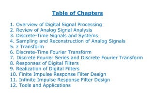
  • 1. Table of Chapters 1. Overview of Digital Signal Processing 2. Review of Analog Signal Analysis 3. Discrete-Time Signals and Systems 4. Sampling and Reconstruction of Analog Signals 5. z Transform 6. Discrete-Time Fourier Transform 7. Discrete Fourier Series and Discrete Fourier Transform 8. Responses of Digital Filters 9. Realization of Digital Filters 10. Finite Impulse Response Filter Design 11. Infinite Impulse Response Filter Design 12. Tools and Applications
  • 2. H. C. So Page 1 Chapter 1: Overview of Digital Signal Processing Chapter Intended Learning Outcomes: (i) Understand basic terminology in digital signal processing (ii) Differentiate digital signal processing and analog signal processing (iii) Describe basic digital signal processing application areas
  • 3. H. C. So Page 2 Signal:  Anything that conveys information, e.g.,  Speech  Electrocardiogram (ECG)  Radar pulse  DNA sequence  Stock price  Code division multiple access (CDMA) signal  Image  Video
  • 4. H. C. So Page 3 0 0.005 0.01 0.015 0.02 -0.6 -0.4 -0.2 0 0.2 0.4 0.6 0.8 time (s) vowel of "a" Fig.1.1: Speech
  • 5. H. C. So Page 4 0 0.5 1 1.5 2 2.5 -50 0 50 100 150 200 250 time (s) ECG Fig.1.2: ECG
  • 6. H. C. So Page 5 0 0.2 0.4 0.6 0.8 1 -1 -0.5 0 0.5 1 time transmitted pulse 0 0.2 0.4 0.6 0.8 1 -1 -0.5 0 0.5 1 time received pulse t Fig.1.3: Transmitted & received radar waveforms
  • 7. H. C. So Page 6 Radar transceiver sends a 1-D sinusoidal pulse at time 0 It then receives echo reflected by an object at a range of Reflected signal is noisy and has a time delay of which corresponds to round trip propagation time of radar pulse Given the signal propagation speed, denoted by , is simply related to as: (1.1) As a result, the radar pulse contains the object range information
  • 8. H. C. So Page 7  Can be a function of one, two or three independent variables, e.g., speech is 1-D signal, function of time; image is 2-D, function of space; wind is 3-D, function of latitude, longitude and elevation  3 types of signals that are functions of time:  Continuous-time (analog) : defined on a continuous range of time , amplitude can be any value  Discrete-time : defined only at discrete instants of time , amplitude can be any value  Digital (quantized) : both time and amplitude are discrete, i.e., it is defined only at and amplitude is confined to a finite set of numbers
  • 9. H. C. So Page 8 quantized signal digital signal processor sample at analog signal sampled signal t amplitude t amplitude 0 0 1 t amplitude 0 1 time and amplitude continuous time discrete amplitude continuous time and amplitude discrete Fig. 1.4: Relationships between , and
  • 10. H. C. So Page 9 at is close to 2 and at and Using 4-bit representation, and , and in general, the value of is restricted to be an integer between and according to the two’s complement representation. In digital signal processing (DSP), we deal with as it corresponds to computer-based processing. Throughout the course, it is assumed that discrete-time signal = digital signal, or the quantizer has infinite resolution
  • 11. H. C. So Page 10 System:  Mathematical model or abstraction of a physical process that relates input to output, e.g.,  Grading system: inputs are coursework and examination marks, output is grade  Squaring system: input is 5, then the output is 25  Amplifier: input is ) cos( t ω , then output is ) cos( 10 t ω  Communication system: input to mobile phone is voice, output from mobile phone is CDMA signal  Noise reduction system: input is a noisy speech, output is a noise-reduced speech  Feature extraction system: input is ) cos( t ω , output is ω  Any system that processes digital signals is called a digital system, digital filter or digital (signal) processor
  • 12. H. C. So Page 11 Processing:  Perform a particular function by passing a signal through system analog signal processor analog input analog output Fig.1.5: Analog processing of analog signal analog-to-digital converter digital signal processor digital-to-analog converter analog input analog output Fig.1.6: Digital processing of analog signal
  • 13. H. C. So Page 12 Advantages of DSP over Analog Signal Processing  Allow development with the use of PC, e.g., MATLAB  Allow flexibility in reconfiguring the DSP operations simply by changing the program  Reliable: processing of 0 and 1 is almost immune to noise and data are easily stored without deterioration  Lower cost due to advancement of VLSI technology  Security can be introduced by encrypting/scrambling  Simple: additions and multiplications are main operations
  • 14. H. C. So Page 13 DSP Application Areas  Speech  Compression (e.g., LPC is a coding standard for compression of speech data)  Synthesis (computer production of speech signals, e.g., text-to-speech engine by Microsoft)  Recognition (e.g., automatic telephone number enquiry system)  Enhancement (e.g., noise reduction for a noisy speech)  Audio  Compression (e.g., MP3 is a coding standard for compression of audio data)
  • 15. H. C. So Page 14  Generation of music by different musical instruments such as piano, cello, guitar and flute using computer  Song with low-cost electronic piano keyboard quality  Automatic music transcription (writing a piece of music down from a recording)  Image and Video  Compression (e.g., JPEG and MPEG is are coding standards for image and video compression, respectively)  Recognition such as face, palm and fingerprint  Enhancement  Construction of 3-D objects from 2-D images  Animation, e.g., “Avatar”
  • 16. H. C. So Page 15  Communications: encoding and decoding of digital communication signals  Astronomy: finding the periods of orbits  Biomedical Engineering: medical care and diagnosis, analysis of ECG, electroencephalogram (EEG), nuclear magnetic resonance (NMR) data  Bioinformatics: DNA sequence analysis, extracting, processing, and interpreting the information contained in genomic and proteomic data  Finance: market risk management, trading algorithm design, investment portfolio analysis
  • 17. H. C. So Page 1 Chapter 2: Review of Analog Signal Analysis Chapter Intended Learning Outcomes: (i) Review of Fourier series which is used to analyze continuous-time periodic signals (ii) Review of Fourier transform which is used to analyze continuous-time aperiodic signals (iii) Review of analog linear time-invariant system
  • 18. H. C. So Page 2 Fourier series and Fourier transform are the tools for analyzing analog signals. Basically, they are used for signal conversion between time and frequency domains: (2.1) Fourier Series  For analysis of continuous-time periodic signals  Express periodic signals using harmonically related sinusoids with frequencies where is called the fundamental frequency  In the frequency domain, only takes discrete values at
  • 19. H. C. So Page 3 continuous and periodic discrete and aperiodic time domain ... ... ... ... frequency domain Fig.2.1: Illustration of Fourier series
  • 20. H. C. So Page 4 A continuous-time function is said to be periodic if there exists such that (2.2) The smallest for which (2.2) holds is called the fundamental period The fundamental frequency is related to as: (2.3) Every periodic function can be expanded into a Fourier series as
  • 21. H. C. So Page 5 (2.4) where , (2.5) are called Fourier series coefficients is characterized by , the Fourier series coefficients in fact correspond to the frequency representation of . Generally, is complex and we use magnitude and phase for its representation
  • 22. H. C. So Page 6 (2.6) and (2.7) Example 2.1 Find the Fourier series coefficients for . It is clear that the fundamental frequency of is . According to (2.3), the fundamental period is thus equal to , which is validated as follows:
  • 23. H. C. So Page 7 With the use of Euler formulas: and we can express as: By inspection and using (2.4), we have while all other Fourier series coefficients are equal to zero
  • 24. H. C. So Page 8 Example 2.2 Find the Fourier series coefficients for . Can we use (2.5)? Why? With the use of Euler formulas, can be written as: Using (2.4), we have:
  • 25. H. C. So Page 9 To plot , we need to compute and for all , e.g., and
  • 26. H. C. So Page 10 Example 2.3 Find the Fourier series coefficients for , which is a periodic continuous-time signal of fundamental period and is a pulse with a width of in each period. Over the specific period from to , is: with . According to (2.3), the fundamental frequency is . Using (2.5), we get:
  • 27. H. C. So Page 11 For : For : The reason of separating the cases of and is to facilitate the computation of , whose value is not straightforwardly obtained from the general expression which involves “0/0”. Nevertheless, using ’s rule:
  • 28. H. C. So Page 12 In summary, if a signal is continuous in time and periodic, we can write: (2.4) The basic steps for finding the Fourier series coefficients are: 1. Determine the fundamental period and fundamental frequency 2. For all , multiply by , then integrate with respect to for one period, finally divide the result by . Usually we separate the calculation into two cases: and
  • 29. H. C. So Page 13 Fourier Transform  For analysis of continuous-time aperiodic signals  Defined on a continuous range of The Fourier transform of an aperiodic and continuous-time signal is: (2.8) which is also called spectrum. The inverse transform is given by (2.9)
  • 30. H. C. So Page 14 continuous and aperiodic continuous and aperiodic time domain frequency domain Fig.2.2: Illustration of Fourier transform
  • 31. H. C. So Page 15 The delta function has the following characteristics: (2.10) (2.11) and (2.12) where is a continuous-time signal. (2.10) and (2.11) indicate that has a very large value or impulse at . That is, is not well defined at (2.12) is known as the sifting property
  • 32. H. C. So Page 16 Fig.2.3: Representation of The unit step function has the form of: (2.13) As there is a sudden change from 0 to 1 at , is not well defined
  • 33. H. C. So Page 17 Example 2.4 Find the Fourier transform of which is a rectangular pulse of the form: Note that the signal is of finite length and corresponds to one period of the periodic function in Example 2.3. Applying (2.8) on yields:
  • 34. H. C. So Page 18 Define the sinc function as: It is seen that is a scaled sinc function because Fig.2.4: Fourier transform pair for rectangular pulse of
  • 35. H. C. So Page 19 Example 2.5 Find the inverse Fourier transform of which is a rectangular pulse of the form: Using (2.9), we get:
  • 36. H. C. So Page 20 Fig.2.5: Fourier transform pair for rectangular pulse of From Examples 2.4 and 2.5, we observe the duality property of Fourier transform Can you guess why we have the duality property? Example 2.6 Find the Fourier transform of with . Employing the property of in (2.13) and (2.8), we get:
  • 37. H. C. So Page 21 Note that when , and Fig.2.6: Magnitude and phase plots for
  • 38. H. C. So Page 22 Example 2.7 Find the Fourier transform of the delta function . Using (2.11) and (2.12) with and , we get: Spectrum of has unit amplitude at all frequencies Based on , Fourier transform can be used to represent continuous-time periodic signals. Consider (2.14)
  • 39. H. C. So Page 23 Taking the inverse Fourier transform of and employing Example 2.7, is computed as: (2.15) As a result, the Fourier transform pair is: (2.16) From (2.4) and (2.16), the Fourier transform pair for a continuous-time periodic signal is: (2.17)
  • 40. H. C. So Page 24 Example 2.8 Find the Fourier transform of which is called an impulse train. Clearly, is a periodic signal with a period of . Using (2.5) and Example 2.7, the Fourier series coefficients are: with . According to (2.17), the Fourier transform is:
  • 41. H. C. So Page 25 ... ... ... ... Fig.2.7: Fourier transform pair for impulse train Fourier transform can be derived from Fourier series: Consider and : ... ... Fig.2.8: Constructing from
  • 42. H. C. So Page 26 is constructed as a periodic version of , with period According to (2.5), the Fourier series coefficients of are: (2.18) where . Noting that for and for , (2.18) can be expressed as: (2.19)
  • 43. H. C. So Page 27 According to (2.8), we can express as: (2.20) The Fourier series expansion for is thus: (2.21) Considering as or and as the area of a rectangle whose height is and width corresponds to the interval of , we obtain (2.22)
  • 44. H. C. So Page 28 Linear Time-Invariant (LTI) System  Linearity: if and are two input-output pairs, then  Time-Invariance: if , then  The input-output relationship for a LTI system is characterized by convolution: (2.23) where , and are input, output and impulse response, respectively  Convolution in time domain corresponds to multiplication in Fourier transform domain, i.e., (2.24)
  • 45. H. C. So Page 29 Proof: The Fourier transform of is (2.25) This suggests that can be computed from inverse Fourier transform of .
  • 46. H. C. So Page 1 Chapter 3: Discrete-Time Signals and Systems Chapter Intended Learning Outcomes: (i) Understanding deterministic and random discrete-time signals and ability to generate them (ii) Ability to recognize the discrete-time system properties, namely, memorylessness, stability, causality, linearity and time-invariance (iii) Understanding discrete-time convolution and ability to perform its computation (iv) Understanding the relationship between difference equations and discrete-time signals and systems
  • 47. H. C. So Page 2 Discrete-Time Signal  Discrete-time signal can be generated using a computing software such as MATLAB  It can also be obtained from sampling continuous-time signals in real world t Fig.3.1:Discrete-time signal obtained from analog signal
  • 48. H. C. So Page 3  The discrete-time signal is equal to only at the sampling interval of , (3.1) where is called the sampling period  is a sequence of numbers, , with being the time index Basic Sequences  Unit Sample (or Impulse) (3.2)
  • 49. H. C. So Page 4 It is similar to the continuous-time unit impulse which is defined in (2.10)-(2.12) is simpler than because it is well defined for all while is not defined at  Unit Step (3.3) It is similar to to the continuous-time of (2.13) is well defined for all but is not defined .
  • 50. H. C. So Page 5 is an important function because it serves as the building block of any discrete-time signal : (3.4) For example, can be expressed in terms of as: (3.5) Conversely, we can use to represent : (3.6)
  • 51. H. C. So Page 6 Introduction to MATLAB  MATLAB stands for ”Matrix Laboratory”  Interactive matrix-based software for numerical and symbolic computation in scientific and engineering applications  Its user interface is relatively simple to use, e.g., we can use the help command to understand the usage and syntax of each MATLAB function  Together with the availability of numerous toolboxes, there are many useful and powerful commands for various disciplines  MathWorks offers MATLAB to C conversion utility  Similar packages include Maple and Mathematica
  • 52. H. C. So Page 7 Discrete-Time Signal Generation using MATLAB A deterministic discrete-time signal satisfies a generating model with known functional form: (3.7) where is a function of parameter vector and time index . That is, given and , can be produced e.g., the time-shifted unit sample and unit step function , where the parameter is e.g., for an exponential function , we have where is the decay factor and is the time shift e.g., for a sinusoid , we have
  • 53. H. C. So Page 8 Example 3.1 Use MATLAB to generate a discrete-time sinusoid of the form: with , , and , which has a duration of 21 samples We can generate by using the following MATLAB code: N=21; %number of samples is 21 A=1; %tone amplitude is 1 w=0.3; %frequency is 0.3 p=1; %phase is 1 for n=1:N x(n)=A*cos(w*(n-1)+p); %time index should be >0 end Note that x is a vector and its index should be at least 1.
  • 54. H. C. So Page 9 Alternatively, we can also use: N=21; %number of samples is 21 A=1; %tone amplitude is 1 w=0.3; %frequency is 0.3 p=1; %phase is 1 n=0:N-1; %define time index vector x=A.*cos(w.*n+p); %first time index is also 1 Both give x = Columns 1 through 7 0.5403 0.2675 -0.0292 -0.3233 -0.5885 -0.8011 -0.9422 Columns 8 through 14 -0.9991 -0.9668 -0.8481 -0.6536 -0.4008 -0.1122 0.1865 Columns 15 through 21 0.4685 0.7087 0.8855 0.9833 0.9932 0.9144 0.7539 Which approach is better? Why?
  • 55. H. C. So Page 10 To plot , we can either use the commands stem(x) and plot(x) If the time index is not specified, the default start time is Nevertheless, it is easy to include the time index vector in the plotting command e.g., Using stem to plot with the correct time index: n=0:N-1; %n is vector of time index stem(n,x) %plot x versus n Similarly, plot(n,x) can be employed to show The MATLAB programs for this example are provided as ex3_1.m and ex3_1_2.m
  • 56. H. C. So Page 11 0 5 10 15 20 -1 -0.8 -0.6 -0.4 -0.2 0 0.2 0.4 0.6 0.8 1 n x[n] Fig.3.2: Plot of discrete-time sinusoid using stem
  • 57. H. C. So Page 12 0 5 10 15 20 -1 -0.8 -0.6 -0.4 -0.2 0 0.2 0.4 0.6 0.8 1 n x[n] Fig.3.3: Plot of discrete-time sinusoid using plot
  • 58. H. C. So Page 13 Apart from deterministic signal, random signal is another importance signal class. It cannot be described by mathematical expressions like deterministic signals but is characterized by its probability density function (PDF). MATLAB has commands to produce two common random signals, namely, uniform and Gaussian (normal) variables. A uniform integer sequence whose values are uniformly distributed between 0 and , can be generated using: (3.8) where and are very large positive integers, is the reminder of dividing by Each admissible value of has the same probability of occurrence of approximately
  • 59. H. C. So Page 14 We also need an initial integer or seed, say, , for starting the generation of (3.8) can be easily modified by properly scaling and shifting e.g., a random number which is uniformly between –0.5 and 0.5, denoted by , is obtained from : (3.9) The MATLAB command rand is used to generate random numbers which are uniformly between 0 and 1 e.g., each realization of stem(0:20,rand(1,21)) gives a distinct and random sequence, with values are bounded between 0 and 1
  • 60. H. C. So Page 15 0 5 10 15 20 0 0.5 1 n 0 5 10 15 20 0 0.5 1 n Fig.3.4: Uniform number realizations using rand
  • 61. H. C. So Page 16 Example 3.2 Use MATLAB to generate a sequence of 10000 random numbers uniformly distributed between –0.5 and 0.5 based on the command rand. Verify its characteristics. According to (3.9), we use u=rand(1,10000)-0.5 to generate the sequence To verify the uniform distribution, we use hist(u,10), which bins the elements of u into 10 equally-spaced containers We see all numbers are bounded between –0.5 and 0.5, and each bar which corresponds to a range of 0.1, contains approximately 1000 elements.
  • 62. H. C. So Page 17 -0.5 0 0.5 0 200 400 600 800 1000 1200 Fig.3.5: Histogram for uniform sequence
  • 63. H. C. So Page 18 On the other hand, the PDF of u, denoted by , is such that . The theoretical mean and power of u, are computed as and Average value and power of u in this realization are computed using mean(u) and mean(u.*u), which give 0.002 and 0.0837, and they align with theoretical calculations
  • 64. H. C. So Page 19 Gaussian numbers can be generated from the uniform variables Given a pair of independent random numbers uniformly distributed between 0 and 1, , a pair of independent Gaussian numbers , which have zero mean and unity power (or variance), can be generated from: (3.10) and (3.11) The MATLAB command is randn. Equations (3.10) and (3.11) are known as the Box-Mueller transformation e.g., each realization of stem(0:20,randn(1,21)) gives a distinct and random sequence, whose values are fluctuating around zero
  • 65. H. C. So Page 20 0 5 10 15 20 -2 0 2 4 n 0 5 10 15 20 -2 -1 0 1 2 n Fig.3.6: Gaussian number realizations using randn
  • 66. H. C. So Page 21 Example 3.3 Use the MATLAB command randn to generate a zero-mean Gaussian sequence of length 10000 and unity power. Verify its characteristics. We use w=randn(1,10000) to generate the sequence and hist(w,50) to show its distribution The distribution aligns with Gaussian variables which is indicated by the bell shape The empirical mean and power of w computed using mean(w) and mean(w.*w) are and 1.0028 The theoretical standard deviation is 1 and we see that most of the values are within –3 and 3
  • 67. H. C. So Page 22 -4 -3 -2 -1 0 1 2 3 4 0 100 200 300 400 500 600 700 Fig.3.7: Histogram for Gaussian sequence
  • 68. H. C. So Page 23 Discrete-Time Systems A discrete-time system is an operator which maps an input sequence into an output sequence : (3.12)  Memoryless: at time depends only on at time Are they memoryless systems? y[n]=(x[n])2 y[n]=x[n]+ x[n-2]  Linear: obey principle of superposition, i.e., if and then (3.13)
  • 69. H. C. So Page 24 Example 3.4 Determine whether the following system with input and output , is linear or not: A standard approach to determine the linearity of a system is given as follows. Let with If , then the system is linear. Otherwise, the system is nonlinear.
  • 70. H. C. So Page 25 Assigning , we have: Note that the outputs for and are and As a result, the system is linear
  • 71. H. C. So Page 26 Example 3.5 Determine whether the following system with input and output , is linear or not: The system outputs for and are and . Assigning , its system output is then: As a result, the system is nonlinear
  • 72. H. C. So Page 27  Time-Invariant: a time-shift of input causes a corresponding shift in output, i.e., if then (3.14) Example 3.6 Determine whether the following system with input and output , is time-invariant or not: A standard approach to determine the time-invariance of a system is given as follows.
  • 73. H. C. So Page 28 Let with If , then the system is time-invariant. Otherwise, the system is time-variant. From the given input-output relationship, is: Let , its system output is: As a result, the system is time-invariant.
  • 74. H. C. So Page 29 Example 3.7 Determine whether the following system with input and output , is time-invariant or not: From the given input-output relationship, is of the form: Let , its system output is: As a result, the system is time-variant.
  • 75. H. C. So Page 30  Causal: output at time depends on input up to time For linear time-invariant (LTI) systems, there is an alternative definition. A LTI system is causal if its impulse response satisfies: (3.15) Are they causal systems? y[n]=x[n]+x[n+1] y[n]=x[n]+x[n-2]  Stable: a bounded input ( ) produces a bounded output ( )
  • 76. H. C. So Page 31 For LTI system, stability also corresponds to (3.16) Are they stable systems? y[n]=x[n]+x[n+1] y[n]=1/x[n] Convolution The input-output relationship for a LTI system is characterized by convolution: (3.17) which is similar to (2.23)
  • 77. H. C. So Page 32 (3.17) is simpler as it only needs additions and multiplications specifies the functionality of the system  Commutative (3.18) and (3.19)
  • 78. H. C. So Page 33 Fig.3.8: Commutative property of convolution
  • 79. H. C. So Page 34  Linearity (3.20) Fig.3.9: Linear property of convolution
  • 80. H. C. So Page 35 Example 3.8 Compute the output if the input is and the LTI system impulse response is . Determine the stability and causality of system. Using (3.17), we have:
  • 81. H. C. So Page 36 Alternatively, we can first establish the general relationship between and with the specific and (3.4): Substituting yields the same . Since and for the system is stable and causal
  • 82. H. C. So Page 37 Example 3.9 Compute the output if the input is and the LTI system impulse response is . Determine the stability and causality of system. Using (3.17), we have:
  • 83. H. C. So Page 38 Let and such that . By employing a change of variable, is expressed as Since for , for . For , is: That is,
  • 84. H. C. So Page 39 Similarly, is: Since for , for . For , is: That is,
  • 85. H. C. So Page 40 Combining the results, we have: or Since , the system is stable. Moreover, the system is causal because for .
  • 86. H. C. So Page 41 Example 3.10 Determine where and are and Here, the lengths of both and are finite. More precisely, , , , , , , and while all other and have zero values.
  • 87. H. C. So Page 42 We still use (3.17) but now it reduces to a finite summation: By considering the non-zero values of , we obtain:
  • 88. H. C. So Page 43 Alternatively, for finite-length discrete-time signals, we can use the MATLAB command conv to compute the convolution of finite-length sequences: n=0:3; x=n.^2+1; h=n+1; y=conv(x,h) The results are y = 1 4 12 30 43 50 40 As the default starting time indices in both h and x are 1, we need to determine the appropriate time index for y
  • 89. H. C. So Page 44 The correct index can be obtained by computing one value of using (3.17). For simplicity, we may compute : In general, if the lengths of and are and , respectively, the length of is .
  • 90. H. C. So Page 45 Linear Constant Coefficient Difference Equations For a LTI system, its input and output are related via a th-order linear constant coefficient difference equation: (3.21) which is useful to check whether a system is both linear and time-invariant or not Example 3.11 Determine if the following input-output relationships correspond to LTI systems: (a) (b) (c)
  • 91. H. C. So Page 46 We see that (a) corresponds to a LTI system with , , and For (b), we reorganize the equation as: which agrees with (3.21) when , and . Hence (b) also corresponds to a LTI system For (c), it does not correspond to a LTI system because and are not linear in the equation Note that if a system cannot be fitted into (3.21), there are three possibilities: linear and time-variant; nonlinear and time-invariant; or nonlinear and time-variant
  • 92. H. C. So Page 47 Example 3.12 Compute the impulse response for a LTI system which is characterized by the following difference equation: Expanding (3.17) as we can easily deduce that only and are nonzero. That is, the impulse response is:
  • 93. H. C. So Page 48 The difference equation is also useful to generate the system output and input. Assuming that , is computed as: (3.22) Assuming that , can be obtained from: (3.23)
  • 94. H. C. So Page 49 Example 3.13 Given a LTI system with difference equation of , compute the system output for with an input of . It is assumed that . The MATLAB code is: N=50; %data length is N+1 y(1)=1; %compute y[0], only x[n] is nonzero for n=2:N+1 y(n)=0.5*y(n-1)+2; %compute y[1],y[2],…,y[50] %x[n]=x[n-1]=1 for n>=1 end n=[0:N]; %set time axis stem(n,y);
  • 95. H. C. So Page 50 0 10 20 30 40 50 0 0.5 1 1.5 2 2.5 3 3.5 4 n y[n] system output Fig.3.10: Output generation with difference equation
  • 96. H. C. So Page 51 Alternatively, we can use the MATLAB command filter by rewriting the equation as: The corresponding MATLAB code is: x=ones(1,51); %define input a=[1,-0.5]; %define vector of a_k b=[1,1]; %define vector of b_k y=filter(b,a,x); %produce output stem(0:length(y)-1,y) The x is the input which has a value of 1 for , while a and b are vectors which contain and , respectively. The MATLAB programs for this example are provided as ex3_13.m and ex3_13_2.m.
  • 97. H. C. So Page 1 Chapter 4: Sampling and Reconstruction of Analog Signals Chapter Intended Learning Outcomes: (i) Ability to convert an analog signal to a discrete-time sequence via sampling (ii) Ability to construct an analog signal from a discrete-time sequence (iii) Understanding the conditions when a sampled signal can uniquely represent its analog counterpart
  • 98. H. C. So Page 2 Sampling  Process of converting a continuous-time signal into a discrete-time sequence  is obtained by extracting every s where is known as the sampling period or interval sample at analog signal discrete-time signal Fig.4.1: Conversion of analog signal to discrete-time sequence  Relationship between and is: (4.1)
  • 99. H. C. So Page 3  Conceptually, conversion of to is achieved by a continuous-time to discrete-time (CD) converter: t n impulse train to sequence conversion CD converter Fig.4.2: Block diagram of CD converter
  • 100. H. C. So Page 4  A fundamental question is whether can uniquely represent or if we can use to reconstruct t Fig.4.3: Different analog signals map to same sequence
  • 101. H. C. So Page 5 But, the answer is yes when: (1) is bandlimited such that its Fourier transform for where is called the bandwidth (2) Sampling period is sufficiently small Example 4.1 The continuous-time signal is used as the input for a CD converter with the sampling period s. Determine the resultant discrete-time signal . According to (4.1), is The frequency in is while that of is
  • 102. H. C. So Page 6 Frequency Domain Representation of Sampled Signal In the time domain, is obtained by multiplying by the impulse train : (4.2) with the use of the sifting property of (2.12) Let the sampling frequency in radian be (or in Hz). From Example 2.8: (4.3)
  • 103. H. C. So Page 7 Using multiplication property of Fourier transform: (4.4) where the convolution operation corresponds to continuous- time signals Using (4.2)-(4.4) and properties of , is:
  • 104. H. C. So Page 8 (4.5) which is the sum of infinite copies of scaled by
  • 105. H. C. So Page 9 When is chosen sufficiently large such that all copies of do not overlap, that is, or , we can get from ... ... ... ... Fig.4.4: for sufficiently large
  • 106. H. C. So Page 10 When is not chosen sufficiently large such that , copies of overlap, we cannot get from , which is referred to aliasing ... ... ... ... Fig.4.5: when is not large enough
  • 107. H. C. So Page 11 Nyquist Sampling Theorem (1928) Let be a bandlimited continuous-time signal with (4.6) Then is uniquely determined by its samples , , if (4.7) The bandwidth is also known as the Nyquist frequency while is called the Nyquist rate and must exceed it in order to avoid aliasing
  • 108. H. C. So Page 12 Application Biomedical Hz 1 kHz Telephone speech kHz 8 kHz Music kHz 44.1 kHz Ultrasonic kHz 250 kHz Radar MHz 200 MHz Table 4.1: Typical bandwidths and sampling frequencies in signal processing applications Example 4.2 Determine the Nyquist frequency and Nyquist rate for the continuous-time signal which has the form of: The frequencies are 0, and . The Nyquist frequency is and the Nyquist rate is
  • 109. H. C. So Page 13 ... ... Fig.4.6: Multiplying and to recover In frequency domain, we multiply by with amplitude and bandwidth with , to obtain , and it corresponds to
  • 110. H. C. So Page 14 Reconstruction  Process of transforming back to sequence to impulse train conversion DC converter Fig.4.7: Block diagram of DC converter From Fig.4.6, is (4.8) where
  • 111. H. C. So Page 15 For simplicity, we set as the average of and : (4.9) To get , we take inverse Fourier transform of and use Example 2.5: (4.10) where
  • 112. H. C. So Page 16 Using (2.23)-(2.24), (4.2) and (2.11)-(2.12), is: (4.11) which holds for all real values of
  • 113. H. C. So Page 17 The interpolation formula can be verified at : (4.12) It is easy to see that (4.13) For , we use ’s rule to obtain: (4.14) Substituting (4.13)-(4.14) into (4.12) yields: (4.15) which aligns with
  • 114. H. C. So Page 18 Example 4.3 Given a discrete-time sequence . Generate its time-delayed version which has the form of where and is a positive integer. Applying (4.11) with : By employing a change of variable of : Is it practical to get y[n]?
  • 115. H. C. So Page 19 Note that when , the time-shifted signal is simply obtained by shifting the sequence by samples: Sampling and Reconstruction in Digital Signal Processing CD converter digital signal processor DC converter Fig.4.8: Ideal digital processing of analog signal  CD converter produces a sequence from  is processed in discrete-time domain to give  DC converter creates from according to (4.11): (4.16)
  • 116. H. C. So Page 20 anti-aliasing filter digital signal processor digital-to-analog converter analog-to-digital converter Fig.4.9: Practical digital processing of analog signal  may not be precisely bandlimited ⇒ a lowpass filter or anti-aliasing filter is needed to process  Ideal CD converter is approximated by AD converter  Not practical to generate  AD converter introduces quantization error  Ideal DC converter is approximated by DA converter because ideal reconstruction of (4.16) is impossible  Not practical to perform infinite summation  Not practical to have future data  and are quantized signals
  • 117. H. C. So Page 21 Example 4.4 Suppose a continuous-time signal is sampled at a sampling frequency of 1000Hz to produce : Determine 2 possible positive values of , say, and . Discuss if or will be obtained when passing through the DC converter. According to (4.1) with s: is easily computed as:
  • 118. H. C. So Page 22 can be obtained by noting the periodicity of a sinusoid: As a result, we have: This is illustrated using the MATLAB code: O1=250*pi; %first frequency O2=2250*pi; %second frequency Ts=1/100000;%successive sample separation is 0.01T t=0:Ts:0.02;%observation interval x1=cos(O1.*t); %tone from first frequency x2=cos(O2.*t); %tone from second frequency There are 2001 samples in 0.02s and interpolating the successive points based on plot yields good approximations
  • 119. H. C. So Page 23 0 5 10 15 20 -1 -0.8 -0.6 -0.4 -0.2 0 0.2 0.4 0.6 0.8 1 n x[n] Fig.4.10: Discrete-time sinusoid
  • 120. H. C. So Page 24 0 0.005 0.01 0.015 0.02 -1 -0.8 -0.6 -0.4 -0.2 0 0.2 0.4 0.6 0.8 1 t Ω 1 Ω 2 Fig.4.11: Continuous-time sinusoids
  • 121. H. C. So Page 25 Passing through the DC converter only produces but not The Nyquist frequency of is and hence the sampling frequency without aliasing is Given Hz or , does not correspond to We can recover because the Nyquist frequency and Nyquist rate for are and Based on (4.11), is: with s
  • 122. H. C. So Page 26 The MATLAB code for reconstructing is: n=-10:30; %add 20 past and future samples x=cos(pi.*n./4); T=1/1000; %sampling interval is 1/1000 for l=1:2000 %observed interval is [0,0.02] t=(l-1)*T/100;%successive sample separation is 0.01T h=sinc((t-n.*T)./T); xr(l)=x*h.'; %approximate interpolation of (4.11) end We compute 2000 samples of in s The value of each at time t is approximated as x*h.' where the sinc vector is updated for each computation The MATLAB program is provided as ex4_4.m
  • 123. H. C. So Page 27 0 0.005 0.01 0.015 0.02 -1 -0.8 -0.6 -0.4 -0.2 0 0.2 0.4 0.6 0.8 1 t x r (t) Fig.4.12: Reconstructed continuous-time sinusoid
  • 124. H. C. So Page 28 Example 4.5 Play the sound for a discrete-time tone using MATLAB. The frequency of the corresponding analog signal is 440 Hz which corresponds to the A note in the American Standard pitch. The sampling frequency is 8000 Hz and the signal has a duration of 0.5 s. The MATLAB code is A=sin(2*pi*440*(0:1/8000:0.5));%discrete-time A sound(A,8000); %DA conversion and play Note that sampling frequency in Hz is assumed for sound. The frequencies of notes B, C#, D, E and F# are 493.88 Hz, 554.37 Hz, 587.33 Hz, 659.26 Hz and 739.99 Hz, respectively. You can easily produce a piece of music with notes: A, A, E, E, F#, F#, E, E, D, D, C#, C#, B, B, A, A.
  • 125. H. C. So Page 1 Chapter 5: z Transform Chapter Intended Learning Outcomes: (i) Understanding the relationship between transform and the Fourier transform for discrete-time signals (ii) Understanding the characteristics and properties of transform (iii) Ability to compute transform and inverse transform (iv) Ability to apply transform for analyzing linear time- invariant (LTI) systems
  • 126. H. C. So Page 2 Definition The transform of , denoted by , is defined as: (5.1) where is a continuous complex variable. Is X(z) real-valued or complex-valued? Relationship with Fourier Transform Employing (4.2), we construct the continuous-time sampled signal with a sampling interval of from : (5.2)
  • 127. H. C. So Page 3 Taking Fourier transform of with using properties of : (5.3) Defining as the discrete-time frequency parameter and writing as , (5.3) becomes (5.4) which is known as discrete-time Fourier transform (DTFT) or Fourier transform of discrete-time signals
  • 128. H. C. So Page 4 is periodic with period : (5.5) where is any integer. Since is a continuous complex variable, we can write (5.6) where is magnitude and is angle of . Employing (5.6), the transform is: (5.7) which is equal to the DTFT of . When or , (5.7) and (5.4) are identical:
  • 129. H. C. So Page 5 (5.8) unit circle -plane Fig.5.1: Relationship between and on the -plane
  • 130. H. C. So Page 6 Region of Convergence (ROC) ROC indicates when transform of a sequence converges Generally there exists some such that (5.9) where the transform does not converge The set of values of for which converges or (5.10) is called the ROC, which must be specified along with in order for the transform to be complete
  • 131. H. C. So Page 7 Assuming that is of infinite length, we decompose : (5.11) where (5.12) and (5.13) Let , is expanded as: (5.14)
  • 132. H. C. So Page 8 According to the ratio test, convergence of requires (5.15) Let . converges if (5.16) That is, the ROC for is .
  • 133. H. C. So Page 9 Let . converges if (5.17) As a result, the ROC for is Combining the results, the ROC for is :  ROC is a ring when  No ROC if and does not exist
  • 134. H. C. So Page 10 -plane -plane -plane -plane Fig.5.2: ROCs for , and Poles and Zeros Values of for which are the zeros of Values of for which are the poles of
  • 135. H. C. So Page 11 In many real-world applications, is represented as a rational function: (5.18) Factorizing and , (5.18) can be written as (5.19) How many poles and zeros in (5.18)? What are they?
  • 136. H. C. So Page 12 Example 5.1 Determine the transform of where is the unit step function. Then determine the condition when the DTFT of exists. Using (5.1) and (3.3), we have According to (5.10), converges if Applying the ratio test, the convergence condition is
  • 137. H. C. So Page 13 Note that we cannot write because may be complex For , is computed as Together with the ROC, the transform of is: It is clear that has a zero at and a pole at . Using (5.8), we substitute to obtain As a result, the existence condition for DTFT of is .
  • 138. H. C. So Page 14 Otherwise, its DTFT does not exist. In general, the DTFT exists if its ROC includes the unit circle. If includes , is required. -plane -plane -plane -plane -plane -plane Fig.5.3: ROCs for and when
  • 139. H. C. So Page 15 Example 5.2 Determine the transform of . Then determine the condition when the DTFT of exists. Using (5.1) and (3.3), we have Similar to Example 5.1, converges if or , which aligns with the ROC for in (5.17). This gives Together with ROC, the transform of is:
  • 140. H. C. So Page 16 Using (5.8), we substitute to obtain As a result, the existence condition for DTFT of is . -plane -plane -plane -plane -plane -plane Fig.5.4: ROCs for and when
  • 141. H. C. So Page 17 Example 5.3 Determine the transform of where . Employing the results in Examples 5.1 and 5.2, we have Note that its ROC agrees with Fig.5.2. What are the pole(s) and zero(s) of X(z)?
  • 142. H. C. So Page 18 Example 5.4 Determine the transform of . Using (5.1) and (3.2), we have Example 5.5 Determine the transform of which has the form of: Using (5.1), we have What are the ROCs in Examples 5.4 and 5.5?
  • 143. H. C. So Page 19 Finite-Duration and Infinite-Duration Sequences Finite-duration sequence: values of are nonzero only for a finite time interval Otherwise, is called an infinite-duration sequence:  Right-sided: if for where is an integer (e.g., with ; with ; with )  Left-sided: if for where is an integer (e.g., with )  Two-sided: neither right-sided nor left-sided (e.g., Example 5.3)
  • 144. H. C. So Page 20 n Fig.5.5: Finite-duration sequences
  • 145. H. C. So Page 21 n Figure 5.6: Infinite-duration sequences
  • 146. H. C. So Page 22 Sequence Transform ROC 1 All , ; , Table 5.1: transforms for common sequences
  • 147. H. C. So Page 23 Eight ROC properties are: P1. There are four possible shapes for ROC, namely, the entire region except possibly and/or , a ring, or inside or outside a circle in the -plane centered at the origin (e.g., Figures 5.5 and 5.6) P2. The DTFT of a sequence exists if and only if the ROC of the transform of includes the unit circle (e.g., Examples 5.1 and 5.2) P3: The ROC cannot contain any poles (e.g., Examples 5.1 to 5.5) P4: When is a finite-duration sequence, the ROC is the entire -plane except possibly and/or (e.g., Examples 5.4 and 5.5)
  • 148. H. C. So Page 24 P5: When is a right-sided sequence, the ROC is of the form where is the pole with the largest magnitude in (e.g., Example 5.1) P6: When is a left-sided sequence, the ROC is of the form where is the pole with the smallest magnitude in (e.g., Example 5.2) P7: When is a two-sided sequence, the ROC is of the form where and are two poles with the successive magnitudes in such that (e.g., Example 5.3) P8: The ROC must be a connected region Example 5.6 A transform contains three poles, namely, , and with . Determine all possible ROCs.
  • 149. H. C. So Page 25 -plane -plane -plane -plane -plane -plane -plane -plane -plane -plane -plane -plane Fig.5.7: ROC possibilities for three poles
  • 150. H. C. So Page 26 What are other possible ROCs? Inverse z Transform Inverse transform corresponds to finding given and its ROC The transform and inverse transform are one-to-one mapping provided that the ROC is given: (5.20) There are 4 commonly used techniques to evaluate the inverse transform. They are 1. Inspection 2. Partial Fraction Expansion 3. Power Series Expansion 4. Cauchy Integral Theorem
  • 151. H. C. So Page 27 Inspection When we are familiar with certain transform pairs, we can do the inverse transform by inspection Example 5.7 Determine the inverse transform of which is expressed as: We first rewrite as:
  • 152. H. C. So Page 28 Making use of the following transform pair in Table 5.1: and putting , we have: By inspection, the inverse transform is:
  • 153. H. C. So Page 29 Partial Fraction Expansion It is useful when is a rational function in : (5.21) For pole and zero determination, it is advantageous to multiply to both numerator and denominator: (5.22)
  • 154. H. C. So Page 30  When , there are pole(s) at  When , there are zero(s) at To obtain the partial fraction expansion from (5.21), the first step is to determine the nonzero poles, There are 4 cases to be considered: Case 1: and all poles are of first order For first-order poles, all are distinct. is: (5.23) For each first-order term of , its inverse transform can be easily obtained by inspection
  • 155. H. C. So Page 31 Multiplying both sides by and evaluating for (5.24) An illustration for computing with is: (5.25) Substituting , we get In summary, three steps are:  Find poles  Find  Perform inverse transform for the fractions by inspection
  • 156. H. C. So Page 32 Example 5.8 Find the pole and zero locations of : Then determine the inverse transform of . We first multiply to both numerator and denominator polynomials to obtain: Apparently, there are two zeros at and . On the other hand, by solving the quadratic equation at the denominator polynomial, the poles are determined as and .
  • 157. H. C. So Page 33 According to (5.23), we have: Employing (5.24), is calculated as: Similarly, is found to be . As a result, the partial fraction expansion for is As the ROC is not specified, we investigate all possible scenarios, namely, , , and .
  • 158. H. C. So Page 34 For , we notice that and where both ROCs agree with . Combining the results, the inverse transform is: which is a right-sided sequence and aligns with P5. For , we make use of and
  • 159. H. C. So Page 35 where both ROCs agree with . This implies: which is a two-sided sequence and aligns with P7. Finally, for : and where both ROCs agree with . As a result, we have: which is a left-sided sequence and aligns with P6.
  • 160. H. C. So Page 36 Suppose is the impulse response of a discrete-time LTI system. Recall (3.15) and (3.16): and The three possible impulse responses:  is the impulse response of a causal but unstable system  corresponds to a noncausal but stable system  is noncausal and unstable Which of the h[n] has/have DTFT?
  • 161. H. C. So Page 37 Case 2: and all poles are of first order In this case, can be expressed as: (5.26)  are obtained by long division of the numerator by the denominator, with the division process terminating when the remainder is of lower degree than the denominator  can be obtained using (5.24). Example 5.9 Determine which has transform of the form:
  • 162. H. C. So Page 38 The poles are easily determined as and According to (5.26) with : The value of is found by dividing the numerator polynomial by the denominator polynomial as follows: That is, . Thus is expressed as
  • 163. H. C. So Page 39 According to (5.24), and are calculated as and With : and the inverse transform is:
  • 164. H. C. So Page 40 Case 3: with multiple-order pole(s) If has a -order pole at with , this means that there are repeated poles with the same value of . is: (5.27)  When there are two or more multiple-order poles, we include a component like the second term for each corresponding pole  can be computed according to (5.24)  can be calculated from: (5.28)
  • 165. H. C. So Page 41 Example 5.10 Determine the partial fraction expansion for : It is clear that corresponds to Case 3 with and one second-order pole at . Hence is: Employing (5.24), is:
  • 166. H. C. So Page 42 Applying (5.28), is: and
  • 167. H. C. So Page 43 Therefore, the partial fraction expansion for is Case 4: with multiple-order pole(s) This is the most general case and the partial fraction expansion of is (5.29) assuming that there is only one multiple-order pole of order at . It is easily extended to the scenarios when there are two or more multiple-order poles as in Case 3. The , and can be calculated as in Cases 1, 2 and 3
  • 168. H. C. So Page 44 Power Series Expansion When is expanded as power series according to (5.1): (5.30) any particular value of can be determined by finding the coefficient of the appropriate power of Example 5.11 Determine which has transform of the form: Expanding yields From (5.30), is deduced as:
  • 169. H. C. So Page 45 Example 5.12 Determine whose transform is given as: With the use of the power series expansion for : with can be expressed as From (5.30), is deduced as:
  • 170. H. C. So Page 46 Example 5.13 Determine whose transform has the form of: With the use of Carrying out long division in with : From (5.30), is deduced as: which agrees with Example 5.1 and Table 5.1
  • 171. H. C. So Page 47 Example 5.14 Determine whose transform has the form of: We first express as: Carrying out long division in with : From (5.30), is deduced as: which agrees with Example 5.2 and Table 5.1
  • 172. H. C. So Page 48 Properties of z Transform 1. Linearity Let and be two transform pairs with ROCs and , respectively, we have (5.31) Its ROC is denoted by , which includes where is the intersection operator. That is, contains at least the intersection of and . Example 5.15 Determine the transform of which is expressed as: where and . By inspection,
  • 173. H. C. So Page 49 the transforms of and are: and According to the linearity property, the transform of is Why the ROC is |z|>0.3 instead of |z|>0.2? 2. Time Shifting A time-shift of in causes a multiplication of in (5.32) The ROC for is basically identical to that of except for the possible addition or deletion of or
  • 174. H. C. So Page 50 Example 5.16 Find the transform of which has the form of: Employing the time-shifting property with and: we easily obtain Note that using (5.1) with also produces the same result but this approach is less efficient:
  • 175. H. C. So Page 51 3. Multiplication by an Exponential Sequence (Modulation) If we multiply by in the time domain, the variable will be changed to in the transform domain. That is: (5.33) If the ROC for is , the ROC for is Example 5.17 With the use of the following transform pair: Find the transform of which has the form of:
  • 176. H. C. So Page 52 Noting that , can be written as: By means of the modulation property of (5.33) with the substitution of and , we obtain: and By means of the linearity property, it follows that which agrees with Table 5.1.
  • 177. H. C. So Page 53 4. Differentiation Differentiating with respect to corresponds to multiplying by in the time domain: (5.34) The ROC for is basically identical to that of except for the possible addition or deletion of or Example 5.18 Determine the transform of . Since and
  • 178. H. C. So Page 54 By means of the differentiation property, we have which agrees with Table 5.1. 5. Conjugation The transform pair for is: (5.35) The ROC for is identical to that of
  • 179. H. C. So Page 55 6. Time Reversal The transform pair for is: (5.36) If the ROC for is , the ROC for is Example 5.19 Determine the transform of Using Example 5.18: and from the time reversal property:
  • 180. H. C. So Page 56 7. Convolution Let and be two transform pairs with ROCs and , respectively. Then we have: (5.37) and its ROC includes . The proof is given as follows. Let (5.38) With the use of the time shifting property, is:
  • 181. H. C. So Page 57 (5.39) Transfer Function of Linear Time-Invariant System A LTI system can be characterized by the transfer function, which is a transform expression
  • 182. H. C. So Page 58 Starting with: (5.40) Applying transform on (5.40) with the use of the linearity and time shifting properties, we have (5.41) The transfer function, denoted by , is defined as: (5.42)
  • 183. H. C. So Page 59 The system impulse response is given by the inverse transform of with an appropriate ROC, that is, , such that . This suggests that we can first take the transforms for and , then multiply by , and finally perform the inverse transform of . Example 5.20 Determine the transfer function for a LTI system whose input and output are related by: Applying transform on the difference equation with the use of the linearity and time shifting properties, is:
  • 184. H. C. So Page 60 Note that there are two ROC possibilities, namely, and and we cannot uniquely determine Example 5.21 Find the difference equation of a LTI system whose transfer function is given by Let . Performing cross-multiplication and inverse transform, we obtain: Examples 5.20 and 5.21 imply the equivalence between the difference equation and transfer function
  • 185. H. C. So Page 61 Example 5.22 Compute the impulse response for a LTI system which is characterized by the following difference equation: Applying transform on the difference equation with the use of the linearity and time shifting properties, is: There is only one ROC possibility, namely, . Taking the inverse transform on , we get: which agrees with Example 3.12
  • 186. H. C. So Page 62 Example 5.23 Determine the output if the input is and the LTI system impulse response is The transforms for and are and As a result, we have: Taking the inverse transform of with the use of the time shifting property yields:
  • 187. H. C. So Page 1 Chapter 6: Discrete-Time Fourier Transform (DTFT) Chapter Intended Learning Outcomes: (i) Understanding the characteristics and properties of DTFT (ii) Ability to perform discrete-time signal conversion between the time and frequency domains using DTFT and inverse DTFT
  • 188. H. C. So Page 2 Definition DTFT is a frequency analysis tool for aperiodic discrete-time signals The DTFT of , , has been derived in (5.4): (6.1) The derivation is based on taking the Fourier transform of of (5.2) As in Fourier transform, is also called spectrum and is a continuous function of the frequency parameter
  • 189. H. C. So Page 3 To convert to , we use inverse DTFT: (6.2) Proof: Putting (6.1) into (6.2) and using (4.13)-(4.14): (6.3)
  • 190. H. C. So Page 4 discrete and aperiodic continuous and periodic time domain frequency domain ... ... Fig.6.1: Illustration of DTFT
  • 191. H. C. So Page 5 is continuous and periodic with a period of is generally complex, we can illustrate using the magnitude and phase spectra, i.e., and : (6.4) and (6.5) where both are continuous in frequency and periodic. Convergence of DTFT The DTFT of a sequence converges if
  • 192. H. C. So Page 6 (6.6) Recall (5.10) and assume the transform of converges for region of convergence (ROC) of : (6.7) When ROC includes the unit circle: (6.8) which leads to the convergence condition for . This also proves the P2 property of the transform.
  • 193. H. C. So Page 7 Let be the impulse response of a linear time-invariant (LTI) system, the following three statements are equivalent: S1. ROC for the transform of includes unit circle S2. The system is stable so that S3. The DTFT of , i.e., , converges Note that is also known as system frequency response Example 6.1 Determine the DTFT of . Using (6.1), the DTFT of is computed as:
  • 194. H. C. So Page 8 Since does not exist. Alternatively, employing the stability condition: which also indicates that the DTFT does not converge
  • 195. H. C. So Page 9 Furthermore, the transform of is: Because does not include the unit circle, there is no DTFT for . Example 6.2 Find the DTFT of . Plot the magnitude and phase spectra for . Using (6.1), we have
  • 196. H. C. So Page 10 Alternatively, we can first use transform because The transform of is evaluated as As the ROC includes the unit circle, its DTFT exists and the same result is obtained by the substitution of . There are two advantages of transform over DTFT:  transform is a generalization of DTFT and it encompasses a broader class of signals since DTFT does not converge for all sequences  notation convenience of writing instead of .
  • 197. H. C. So Page 11 To plot the magnitude and phase spectra, we express : In doing so, and can be written in closed- forms as: and Note that we generally employ (6.4) and (6.5) for magnitude and phase computation
  • 198. H. C. So Page 12 In using MATLAB to plot and , we utilize the command sinc so that there is no need to separately handle the “0/0” cases due to the sine functions Recall the definition of sinc function: As a result, we have:
  • 199. H. C. So Page 13 The key MATLAB code for is N=10; %N=10 w=0:0.01*pi:2*pi; %successive frequency point %separation is 0.01pi dtft=N.*sinc(w.*N./2./pi)./(sinc(w./2./pi)).*exp(- j.*w.*(N-1)./2); %define DTFT function subplot(2,1,1) Mag=abs(dtft); %compute magnitude plot(w./pi,Mag); %plot magnitude subplot(2,1,2) Pha=angle(dtft); %compute phase plot(w./pi,Pha); %plot phase Analogous to Example 4.4, there are 201 uniformly-spaced points to approximate the continuous functions and .
  • 200. H. C. So Page 14 0 0.5 1 1.5 2 0 5 10 Magnitude Response ω/p 0 0.5 1 1.5 2 -4 -2 0 2 4 Phase Response ω/p Fig.6.2: DTFT plots using abs and angle
  • 201. H. C. So Page 15 Alternatively, we can use the command freqz: which is ratio of two polynomials in The corresponding MATLAB code is: N=10; %N=10 a=[1,-1]; %vector for denominator b=[1,zeros(1,N-1),-1]; %vector for numerator freqz(b,a) %plot magnitude & phase (dB) Note that it is also possible to use and in this case we have b=ones(N,1) and a=1.
  • 202. H. C. So Page 16 0 0.2 0.4 0.6 0.8 1 -200 -100 0 100 Normalized Frequency (×π rad/samπle) Phase (degrees) 0 0.2 0.4 0.6 0.8 1 -60 -40 -20 0 20 Normalized Frequency (×π rad/samπle) Magnitude (dB) Fig.6.3: DTFT plots using freqz
  • 203. H. C. So Page 17 The results in Figs. 6.2 and 6.3 are identical, although their presentations are different:  at in Fig. 6.2 while that of Fig. 6.3 is 20 dB. It is easy to verify that 10 corresponds to dB  units of phase spectra in Figs. 6.2 and 6.3 are radian and degree, respectively. To make the phase values in both plots identical, we also need to take care of the phase ambiguity. The MATLAB programs for this example are provided as ex6_2.m and ex6_2_2.m.
  • 204. H. C. So Page 18 Example 6.3 Find the inverse DTFT of which is a rectangular pulse within : where . Using (6.2), we get: That is, is an infinite-duration sequence whose values are drawn from a scaled sinc function.
  • 205. H. C. So Page 19 Example 6.4 Determine the inverse DTFT of which has the form of: With the use of , the corresponding transform is Note that ROC should include the unit circle as DTFT exists Employing the time shifting property, we get
  • 206. H. C. So Page 20 Properties of DTFT Since DTFT is closely related to transform, its properties follow those of transform. Note that ROC is not involved because it should include unit circle in order for DTFT exists 1. Linearity If and are two DTFT pairs, then: (6.9) 2. Time Shifting A shift of in causes a multiplication of in : (6.10)
  • 207. H. C. So Page 21 3. Multiplication by an Exponential Sequence Multiplying by in time domain corresponds to a shift of in the frequency domain: (6.11) which agrees with (5.33) by putting and 4. Differentiation Differentiating with respect to corresponds to multiplying by : (6.12)
  • 208. H. C. So Page 22 Note the RHS is obtained from (5.34) by putting : (6.13) 5. Conjugation The DTFT pair for is given as: (6.14) 6. Time Reversal The DTFT pair for is given as: (6.15)
  • 209. H. C. So Page 23 7. Convolution If and are two DTFT pairs, then: (6.16) In particular, for a LTI system with input , output and impulse response , we have: (6.17) which is analogous to (2.24) for continuous-time LTI systems
  • 210. H. C. So Page 24 8. Multiplication Multiplication in the time domain corresponds to convolution in the frequency domain: (6.18) where denotes convolution within one period 9. Parseval’s Relation The Parseval’s relation addresses the energy of a sequence: (6.19)
  • 211. H. C. So Page 25 With the use of (6.2), the proof is: (6.20)
  • 212. H. C. So Page 1 Chapter 7: Discrete Fourier Series & Discrete Fourier Transform Chapter Intended Learning Outcomes (i) Understanding the relationships between the transform, discrete-time Fourier transform (DTFT), discrete Fourier series (DFS) and discrete Fourier transform (DFT) (ii) Understanding the characteristics and properties of DFS and DFT (iii) Ability to perform discrete-time signal conversion between the time and frequency domains using DFS and DFT and their inverse transforms
  • 213. H. C. So Page 2 Discrete Fourier Series DTFT may not be practical for analyzing because is a function of the continuous frequency variable and we cannot use a digital computer to calculate a continuum of functional values DFS is a frequency analysis tool for periodic infinite-duration discrete-time signals which is practical because it is discrete in frequency The DFS is derived from the Fourier series as follows. Let be a periodic sequence with fundamental period where is a positive integer. Analogous to (2.2), we have: (7.1) for any integer value of .
  • 214. H. C. So Page 3 Let be the continuous-time counterpart of . According to Fourier series expansion, is: (7.2) which has frequency components at . Substituting , and : (7.3) Note that (7.3) is valid for discrete-time signals as only the sample points of are considered. It is seen that has frequency components at and the respective complex exponentials are .
  • 215. H. C. So Page 4 Nevertheless, there are only distinct frequencies in due to the periodicity of . Without loss of generality, we select the following distinct complex exponentials, , and thus the infinite summation in (7.3) is reduced to: (7.4) Defining , , as the DFS coefficients, the inverse DFS formula is given as: (7.5)
  • 216. H. C. So Page 5 The formula for converting to is derived as follows. Multiplying both sides of (7.5) by and summing from to : (7.6) Using the orthogonality identity of complex exponentials: (7.7)
  • 217. H. C. So Page 6 (7.6) is reduced to (7.8) which is also periodic with period . Let (7.9) The DFS analysis and synthesis pair can be written as: (7.10) and (7.11)
  • 218. H. C. So Page 7 discrete and periodic discrete and periodic time domain frequency domain ... ... ... ... Fig.7.1: Illustration of DFS
  • 219. H. C. So Page 8 Example 7.1 Find the DFS coefficients of the periodic sequence with a period of . Plot the magnitudes and phases of . Within one period, has the form of: Using (7.10), we have
  • 220. H. C. So Page 9 Similar to Example 6.2, we get: and The key MATLAB code for plotting DFS coefficients is N=5; x=[1 1 1 0 0]; k=-N:2*N; %plot for 3 periods Xm=abs(1+2.*cos(2*pi.*k/N));%magnitude computation Xa=angle(exp(-2*j*pi.*k/5).*(1+2.*cos(2*pi.*k/N))); %phase computation The MATLAB program is provided as ex7_1.m.
  • 221. H. C. So Page 10 -5 0 5 10 0 1 2 3 Magnitude Response k -5 0 5 10 -2 -1 0 1 2 Phase Response k Fig.7.2: DFS plots
  • 222. H. C. So Page 11 Relationship with DTFT Let be a finite-duration sequence which is extracted from a periodic sequence of period : (7.12) Recall (6.1), the DTFT of is: (7.13) With the use of (7.12), (7.13) becomes (7.14)
  • 223. H. C. So Page 12 Comparing the DFS and DTFT in (7.8) and (7.14), we have: (7.15) That is, is equal to sampled at distinct frequencies between with a uniform frequency spacing of . Samples of or DTFT of a finite-duration sequence can be computed using the DFS of an infinite-duration periodic sequence , which is a periodic extension of .
  • 224. H. C. So Page 13 Relationship with z Transform is also related to transform of according to (5.8): (7.16) Combining (7.15) and (7.16), is related to as: (7.17) That is, is equal to evaluated at equally-spaced points on the unit circle, namely, .
  • 225. H. C. So Page 14 unit circle -plane . . . . . . Fig.7.3: Relationship between , and
  • 226. H. C. So Page 15 Example 7.2 Determine the DTFT of a finite-duration sequence : Then compare the results with those in Example 7.1. Using (6.1), the DTFT of is computed as:
  • 227. H. C. So Page 16 -2 -1 0 1 2 3 4 0 1 2 3 Magnitude Response ω/p -2 -1 0 1 2 3 4 -2 -1 0 1 2 Phase Response ω/p Fig.7.4: DTFT plots
  • 228. H. C. So Page 17 -2 -1 0 1 2 3 4 0 1 2 3 Magnitude Response ω/p -2 -1 0 1 2 3 4 -2 0 2 Phase Response ω/p Fig.7.5: DFS and DTFT plots with
  • 229. H. C. So Page 18 Suppose in Example 7.1 is modified as: Via appending 5 zeros in each period, now we have . What is the period of the DFS? What is its relationship with that of Example 7.2? How about if infinite zeros are appended? The MATLAB programs are provided as ex7_2.m, ex7_2_2.m and ex7_2_3.m.
  • 230. H. C. So Page 19 -2 -1 0 1 2 3 4 0 1 2 3 Magnitude Response ω/p -2 -1 0 1 2 3 4 -2 -1 0 1 2 Phase Response ω/p Fig.7.6: DFS and DTFT plots with
  • 231. H. C. So Page 20 Properties of DFS 1. Periodicity If is a periodic sequence with period , its DFS is also periodic with period : (7.18) where is any integer. The proof is obtained with the use of (7.10) and as follows: (7.19)
  • 232. H. C. So Page 21 2. Linearity Let and be two DFS pairs with the same period of . We have: (7.20) 3. Shift of Sequence If , then (7.21) and (7.22) where is the period while and are any integers. Note that (7.21) follows (6.10) by putting and (7.22) follows (6.11) via the substitution of .
  • 233. H. C. So Page 22 4. Duality If , then (7.23) 5. Symmetry If , then (7.24) and (7.25) Note that (7.24) corresponds to the DTFT conjugation property in (6.14) while (7.25) is similar to the time reversal property in (6.15).
  • 234. H. C. So Page 23 6. Periodic Convolution Let and be two DFS pairs with the same period of . We have (7.26) Analogous to (6.18), denotes discrete-time convolution within one period. With the use of (7.11) and (7.21), the proof is given as follows:
  • 235. H. C. So Page 24 (7.27) To compute where both and are of period , we indeed only need the samples with .
  • 236. H. C. So Page 25 Let . Expanding (7.26), we have: (7.28) For : (7.29) For : (7.30)
  • 237. H. C. So Page 26 A period of can be computed in matrix form as: (7.31) Example 7.3 Given two periodic sequences and with period : and Compute .
  • 238. H. C. So Page 27 Using (7.31), is computed as: The square matrix can be determined using the MATLAB command toeplitz([1,2,3,4],[1,4,3,2]). That is, we only need to know its first row and first column.
  • 239. H. C. So Page 28 Periodic convolution can be utilized to compute convolution of finite-duration sequences in (3.17) as follows. Let and be finite-duration sequences with lengths and , respectively, and which has a length of We append and zeros at the ends of and for constructing periodic and where both are of period is then obtained from one period of . Example 7.4 Compute the convolution of and with the use of periodic convolution. The lengths of and are 2 and 3 with , , , and .
  • 240. H. C. So Page 29 The length of is 4. As a result, we append two zeros and one zero in and , respectively. According to (7.31), the MATLAB code is: toeplitz([1,-4,5,0],[1,0,5,-4])*[2;3;0;0] which gives 2 -5 -2 15 Note that the command conv([2,3],[1,-4,5]) also produces the same result.
  • 241. H. C. So Page 30 Discrete Fourier Transform DFT is used for analyzing discrete-time finite-duration signals in the frequency domain Let be a finite-duration sequence of length such that outside . The DFT pair of is: (7.32) and (7.33)
  • 242. H. C. So Page 31 If we extend to a periodic sequence with period , the DFS pair for is given by (7.10)-(7.11). Comparing (7.32) and (7.10), for . As a result, DFT and DFS are equivalent within the interval of Example 7.5 Find the DFT coefficients of a finite-duration sequence which has the form of Using (7.32) and Example 7.1 with , we have:
  • 243. H. C. So Page 32 Together with whose index is outside the interval of , we finally have: If the length of is considered as such that , then we obtain:
  • 244. H. C. So Page 33 The MATLAB command for DFT computation is fft. The MATLAB code to produce magnitudes and phases of is: N=5; x=[1 1 1 0 0]; %append 2 zeros subplot(2,1,1); stem([0:N-1],abs(fft(x))); %plot magnitude response title('Magnitude Response'); subplot(2,1,2); stem([0:N-1],angle(fft(x)));%plot phase response title('Phase Response'); According to Example 7.2 and the relationship between DFT and DFS, the DFT will approach the DTFT when we append infinite zeros at the end of The MATLAB program is provided as ex7_5.m.
  • 245. H. C. So Page 34 0 1 2 3 4 0 1 2 3 Magnitude Response 0 1 2 3 4 -2 -1 0 1 2 Phase Response Fig.7.7: DFT plots with
  • 246. H. C. So Page 35 Example 7.6 Given a discrete-time finite-duration sinusoid: Estimate the tone frequency using DFT. Consider the continuous-time case first. According to (2.16), Fourier transform pair for a complex tone of frequency is: That is, can be found by locating the peak of the Fourier transform. Moreover, a real-valued tone is:
  • 247. H. C. So Page 36 From the Fourier transform of , and are located from the two impulses. Analogously, there will be two peaks which correspond to frequencies and in the DFT for . The MATLAB code is N=21; %number of samples is 21 A=2; %tone amplitude is 2 w=0.7*pi; %frequency is 0.7*pi p=1; %phase is 1 n=0:N-1; %define a vector of size N x=A*cos(w*n+p); %generate tone X=fft(x); %compute DFT subplot(2,1,1); stem(n,abs(X)); %plot magnitude response subplot(2,1,2); stem(n,angle(X)); %plot phase response
  • 248. H. C. So Page 37 0 5 10 15 20 0 5 10 15 20 Magnitude Response 0 5 10 15 20 -2 -1 0 1 2 Phase Response Fig.7.8: DFT plots for a real tone
  • 249. H. C. So Page 38 X = 1.0806 1.0674+0.2939i 1.0243+0.6130i 0.9382+0.9931i 0.7756+1.5027i 0.4409+2.3159i -0.4524+4.1068i -6.7461+15.1792i 6.5451-7.2043i 3.8608-2.1316i 3.3521-0.5718i 3.3521+0.5718i 3.8608+2.1316i 6.5451+7.2043i -6.7461-15.1792i -0.4524-4.1068i 0.4409-2.3159i 0.7756-1.5027i 0.9382-0.9931i 1.0243-0.6130i 1.0674-0.2939i Interestingly, we observe that and . In fact, all real-valued sequences possess these properties so that we only have to compute around half of the DFT coefficients. As the DFT coefficients are complex-valued, we search the frequency according to the magnitude plot.
  • 250. H. C. So Page 39 There are two peaks, one at and the other at which correspond to and , respectively. From Example 7.2, it is clear that the index refers to . As a result, an estimate of is: To improve the accuracy, we append a large number of zeros to . The MATLAB code for is now modified as: x=[A*cos(w.*n+p) zeros(1,1980)]; where 1980 zeros are appended. The MATLAB code is provided as ex7_6.m and ex7_6_2.m.
  • 251. H. C. So Page 40 0 500 1000 1500 2000 0 5 10 15 20 25 Magnitude Response 0 500 1000 1500 2000 -4 -2 0 2 4 Phase Response Fig.7.9: DFT plots for a real tone with zero padding
  • 252. H. C. So Page 41 The peak index is found to be with . Thus Example 7.7 Find the inverse DFT coefficients for which has a length of and has the form of Plot . Using (7.33) and Example 7.5, we have:
  • 253. H. C. So Page 42 The main MATLAB code is: N=5; X=[1 1 1 0 0]; subplot(2,1,1); stem([0:N-1],abs(ifft(X))); subplot(2,1,2); stem([0:N-1],angle(ifft(X))); The MATLAB program is provided as ex7_7.m.
  • 254. H. C. So Page 43 0 1 2 3 4 0 0.2 0.4 Magnitude Response 0 1 2 3 4 -2 -1 0 1 2 Phase Response Fig.7.10: Inverse DFT plots
  • 255. H. C. So Page 44 Properties of DFT Since DFT pair is equal to DFS pair within , their properties will be identical if we take care of the values of and when the indices are outside the interval 1. Linearity Let and be two DFT pairs with the same duration of . We have: (7.34) Note that if and are of different lengths, we can properly append zero(s) to the shorter sequence to make them with the same duration.
  • 256. H. C. So Page 45 2. Circular Shift of Sequence If , then (7.35) Note that in order to make sure that the resultant time index is within the interval of , we need circular shift, which is defined as (7.36) where the integer is chosen such that (7.37)
  • 257. H. C. So Page 46 Example 7.8 Determine where is of length 4 and has the form of: According to (7.36)-(7.37) with , is determined as:
  • 258. H. C. So Page 47 3. Duality If , then (7.38) 4. Symmetry If , then (7.39) and (7.40)
  • 259. H. C. So Page 48 5. Circular Convolution Let and be two DFT pairs with the same duration of . We have (7.41) where is the circular convolution operator.
  • 260. H. C. So Page 49 Fast Fourier Transform FFT is a fast algorithm for DFT and inverse DFT computation. Recall (7.32): (7.42) Each involves and complex multiplications and additions, respectively. Computing all DFT coefficients requires complex multiplications and complex additions. Assuming that , the corresponding computational requirements for FFT are complex multiplications and complex additions.
  • 261. H. C. So Page 50 Direct Computation FFT Multiplication Addition Multiplication Addition 2 4 2 1 2 8 64 56 12 24 32 1024 922 80 160 64 4096 4022 192 384 1048576 1047552 5120 10240 ~ ~ ~ ~ Table 7.1: Complexities of direct DFT computation and FFT
  • 262. H. C. So Page 51 Basically, FFT makes use of two ideas in its development:  Decompose the DFT computation of a sequence into successively smaller DFTs  Utilize two properties of : complex conjugate symmetry property: (7.43) periodicity in and : (7.44)
  • 263. H. C. So Page 52 Decimation-in-Time Algorithm The basic idea is to compute (7.42) according to (7.45) Substituting and for the first and second summation terms: (7.46)
  • 264. H. C. So Page 53 Using since , we have: (7.47) where and are the DFTs of the even-index and odd- index elements of , respectively. That is, can be constructed from two -point DFTs, namely, and . Further simplifications can be achieved by writing the equations as 2 groups of equations as follows: (7.48) and
  • 265. H. C. So Page 54 (7.49) with the use of and . Equations (7.48) and (7.49) are known as the butterfly merging equations. Noting that multiplications are also needed to calculate , the number of multiplications is reduced from to . The decomposition step of (7.48)-(7.49) is repeated times until 1-point DFT is reached.
  • 266. H. C. So Page 55 Decimation-in-Frequency Algorithm The basic idea is to decompose the frequency-domain sequence into successively smaller subsequences. Recall (7.42) and employing and , the even-index DFT coefficients are: (7.50)
  • 267. H. C. So Page 56 Using and , the odd-index coefficients are: (7.51) and are equal to -point DFTs of and , respectively. The decomposition step of (7.50)-(7.51) is repeated times until 1-point DFT is reached.
  • 268. H. C. So Page 1 Chapter 8: Responses of Digital Filters Chapter Intended Learning Outcomes: (i) Understanding the relationships between impulse response, frequency response, difference equation and transfer function in characterizing a LTI system (ii) Ability to identify infinite impulse response (IIR) and finite impulse response (FIR) filters. Note that a digital filter is system which processes discrete-time signals (iii) Ability to compute system frequency response
  • 269. H. C. So Page 2 LTI System Characterization CD converter discrete-time LTI system DC converter Fig.8.1: Processing of analog signal with LTI filter The LTI system can be characterized as  Impulse Response Let be the impulse response of the LTI filter. Recall from (3.17), it characterizes the system via the convolution: (8.1) is the time-domain response of the LTI filter
  • 270. H. C. So Page 3  Frequency Response We have from (6.17), which is the discrete-time Fourier transform (DTFT) of (8.1): (8.2) is the frequency-domain response of the LTI filter  Difference Equation A LTI system satisfies a difference equation of the form: (8.3)
  • 271. H. C. So Page 4  Transfer Function Taking the transform on both sides of (8.3): (8.4) Which of them can uniquely characterize a system? Which of them cannot?
  • 272. H. C. So Page 5 Example 8.1 Given the difference equation with input and output : Find all possible ways to compute given . In fact, there are two ways to compute . A straightforward and practical way is to implement a causal system by using the difference equation recursively with a given initial condition of :
  • 273. H. C. So Page 6 On the other hand, it is possible to implement a noncausal system via reorganizing the difference equation as: In doing so, we need an initial future value of and future inputs, and the recursive implementation is: As a result, generally the difference equation cannot uniquely characterize the system.
  • 274. H. C. So Page 7 Nevertheless, if causality is assumed, then the difference equation corresponds to a unique LTI system. Alternatively, we can also study the computation of using system transfer function : Since the ROC is not specified, there are two possible cases, namely, and . For or , using inverse transform:
  • 275. H. C. So Page 8 which corresponds to a causal system. The same result can also be produced by first finding the system impulse response via inverse transform of : and then computing .
  • 276. H. C. So Page 9 For or , using inverse transform: which corresponds to a noncausal system. Example 8.2 Discuss all possibilities for the LTI system whose input and output are related by:
  • 277. H. C. So Page 10 Taking transform on the difference equation yields: There are 3 possible choices: : The ROC is outside the circle with radius characterized by the largest-magnitude pole. The system can be causal but is not stable since the ROC does not include the unit circle : The system is stable because the ROC includes the unit circle but not causal : The system is unstable and noncausal
  • 278. H. C. So Page 11 Impulse Response of Digital Filters When is a rational function of with only first-order poles, we have from (5.26): (8.5) where the first component is present only if . If the system is causal, then the ROC must be of the form where is the largest-magnitude pole.
  • 279. H. C. So Page 12 According to this ROC, the impulse response is: (8.6) There are two possible cases for (8.6) which correspond to IIR and FIR filters:  IIR Filter If or there is at least one pole, the system is referred to as an IIR filter because is of infinite duration.  FIR Filter If or there is no pole, the system is referred to as a FIR filter because is of finite duration.
  • 280. H. C. So Page 13 Notice that the definitions of IIR and FIR systems also hold for noncausal systems. Example 8.3 Determine if the following difference equations correspond to IIR or FIR systems. All systems are assumed causal. (a) (b) Taking the transform on (a) yields which has one pole. For causal system:
  • 281. H. C. So Page 14 which is a right-sided sequence and corresponds to an IIR system as is of infinite duration. Similarly, we have for (b): which does not have any nonzero pole. Hence which corresponds to a FIR system as is of finite duration.
  • 282. H. C. So Page 15 Frequency Response of Digital Filters The frequency response of a LTI system whose impulse response is obtained by taking the DTFT of : (8.7) According to (5.8), is also obtained if is available: (8.8) assuming that the ROC of includes the unit circle.
  • 283. H. C. So Page 16 Example 8.4 Plot the frequency response of the system with impulse response of the form: where Following Example 7.6, we append a large number of zeros at the end of prior to performing discrete Fourier transform (DFT) to produce more DTFT samples. Is it a low-pass filter? Why? The MATLAB program is provided as ex8_4.m.
  • 284. H. C. So Page 17 0 0.5 1 1.5 2 0 5 10 Magnitude Response ω/p 0 0.5 1 1.5 2 -4 -2 0 2 4 Phase Response ω/p Fig.8.2: Frequency response for sinc
  • 285. H. C. So Page 18 Example 8.5 Plot the frequency response of the system with transfer function of the form: It is assumed that the ROC of includes the unit circle. The MATLAB code is b=[1,2,3]; a=[2,3,4]; freqz(b,a); Is it a lowpass filter? Why? The MATLAB program is provided as ex8_5.m.
  • 286. H. C. So Page 19 0 0.2 0.4 0.6 0.8 1 -20 -10 0 10 20 Normalized Frequency (×π rad/samπle) Phase (degrees) 0 0.2 0.4 0.6 0.8 1 -4 -3 -2 -1 0 Normalized Frequency (×π rad/samπle) Magnitude (dB) Fig.8.3: Frequency response for second-order system
  • 287. H. C. So Page 1 Chapter 9: Realization of Digital Filters Chapter Intended Learning Outcomes: (i) Ability to implement finite impulse response (FIR) and infinite impulse response (IIR) filters using different structures in terms of block diagram and signal flow graph (ii) Ability to determine the system transfer function and difference equation given the corresponding block diagram or signal flow graph representation.
  • 288. H. C. So Page 2 Filter Implementation When causality is assumed, a LTI filter can be uniquely characterized by its transfer function : (9.1) or the corresponding difference equation: (9.2) where and are the system input and output
  • 289. H. C. So Page 3 Assuming , the output is: (9.3) Assigning and yields (9.4) Computing involves and . That is, we need  Delay elements or storage  Multipliers  Adders (subtraction is considered as addition)
  • 290. H. C. So Page 4 How many storage elements are needed? How many multipliers are needed? How many adders are needed? Computations of ] [n y can be arranged in different ways to give the same difference equation, which leads to different structures for realization of discrete-time LTI systems 4 basic forms of implementations, namely, direct form, canonic form, cascade form and parallel form will be described An implementation can be represented using either a block diagram or a signal flow graph
  • 291. H. C. So Page 5 Block Diagram Representation adder multiplier unit delay Fig.9.1: Basic operations in block diagram
  • 292. H. C. So Page 6 Although an adder can generally deal with more than two sequences, here we consider two signals in order to align with practical implementation in microprocessors. When , it corresponds to signal amplification while the signal is attenuated for . Note that a multiplier usually has the highest implementation or computational cost and thus it is desired to reduce the number of multipliers in different systems, if possible. The transfer function corresponds to a unit delay. It can be implemented by providing a storage register for each unit delay in digital implementation. If the required number of samples of delay is , then the corresponding system function is .
  • 293. H. C. So Page 7 Signal Flow Graph Representation adder multiplier unit delay Figure 9.2: Basic operations in signal flow graph
  • 294. H. C. So Page 8 Its basic elements are branches with directions, and nodes. That is, a signal flow graph is a set of directed branches that connect at nodes. Signal at a node of a flow graph is equal to the sum of the signals from all branches connecting to the node. Signal out of a branch is equal to the branch gain times the signal into the branch. Branch gain can refer to a scalar or a transfer function of corresponding to multiplication or unit delay operation, respectively. When the branch gain is unity, it is left unlabeled. A signal flow graph provides an alternative but equivalent graphical representation to a block diagram structure
  • 295. H. C. So Page 9 Example 9.1 Draw the block diagram and signal flow graph representations of a LTI system whose input and output satisfy the following difference equation: Fig.9.3: Illustration of block diagram
  • 296. H. C. So Page 10 Fig.9.4: Illustration of signal flow graph 2 adders, 3 multipliers and 2 delay elements are required to implement the system.
  • 297. H. C. So Page 11 Structures for FIR Filter For FIR filter, its transfer function does not contain pole. That is, setting and in (9.1) yields a FIR system: (9.5) while the corresponding difference equation is: (9.6)
  • 298. H. C. So Page 12 1. Direct Form Comparing (9.6) with the convolution formula of (3.18), correspond to the system impulse response : (9.7) (9.6) can also be written as: (9.8) The direct form follows straightforwardly from the difference equation.
  • 299. H. C. So Page 13 The implementation needs memory locations for storing previous inputs of , multiplications and additions for computing each output value of . Fig.9.5: Direct form of FIR filter
  • 300. H. C. So Page 14 2. Cascade Form Expressing (9.5) as products of second-order polynomial system functions via factorization: (9.9) where is the largest integer contained in . Note that when is odd, one of the will be zero. Assuming that is even, this implementation needs storage elements, multiplications and additions, for computing each output value of . Why second-order polynomial instead of first-order polynomial?
  • 301. H. C. So Page 15 Fig.9.6: Cascade form of FIR filter (9.10) and (9.11)
  • 302. H. C. So Page 16 Taking transform on (9.10) and (9.11): (9.12) and (9.13) Substituting (9.13) into (9.12) yields: (9.14) Extending (9.14) to , we finally get: (9.15)
  • 303. H. C. So Page 17 To save the computational complexity, we express (9.9) as: (9.16) where , and , . That is, all are normalized to 1. Assuming that is even, (9.16) needs delay elements, multiplications and additions, for computing each output value of
  • 304. H. C. So Page 18 Fig.9.7: Cascade form of FIR filter with smaller complexity Example 9.2 Draw the signal flow graph using the cascade form for the LTI system whose transfer function is:
  • 305. H. C. So Page 19 To factorize , we use the MATLAB command roots([1 1 1 1 1]) to solve for the roots: 0.3090 + 0.9511i 0.3090 - 0.9511i -0.8090 + 0.5878i -0.8090 - 0.5878i Hence can be factorized as Although it can be realized with first-order sections, complex coefficients are needed, which implies higher computational cost. To guarantee real-valued coefficients, we group the sections of complex conjugates together:
  • 306. H. C. So Page 20 Fig.9.8: Two possible cascade forms for FIR filter
  • 307. H. C. So Page 21 Structures for IIR Filter When there is at least one pole in , it corresponds to an IIR filter. The corresponding transfer function is thus: (9.17) That is, IIR filter is the general form of any discrete-time LTI system.
  • 308. H. C. So Page 22 1. Direct Form It realizes (9.4) in an explicit manner via decomposing it into a pair of difference equations: (9.18) and (9.19) The direct form can also be obtained by decomposing into two transfer functions as: (9.20) where
  • 309. H. C. So Page 23 (9.21) and (9.22) In the transform domain, we have: (9.23) and (9.24)
  • 310. H. C. So Page 24 Fig.9.9: Direct form of IIR filter
  • 311. H. C. So Page 25 The direct form implementation needs memory locations, multiplications and additions, for computing each output value of . 2. Canonic Form On the other hand, we can first pass through the filter to produce an intermediate signal . The is then passed through the system to give : (9.25) and (9.26)
  • 312. H. C. So Page 26 Applying inverse transform, we get: (9.27) and (9.28) which can be considered as an alternative direct form.
  • 313. H. C. So Page 27 Fig.9.10: Alternative direct form of IIR filter
  • 314. H. C. So Page 28 Assume . Since the same signals , are stored in the two chains of storage elements, they can be combined to reduce the memory requirement. In general, the minimum number of delay elements required is . It is called canonic form because this implementation involves the minimum number of storages.
  • 315. H. C. So Page 29 Fig.9.11: Canonic form of IIR filter
  • 316. H. C. So Page 30 Example 9.3 Draw the block diagrams using the direct and canonic forms for the LTI system whose transfer function is: According to (9.18)-(9.19): Based on (9.27)-(9.28):
  • 317. H. C. So Page 31 Fig.9.12: Direct form of second-order IIR filter Fig.9.13: Canonic form of second-order IIR filter
  • 318. H. C. So Page 32 3. Cascade Form We factorize the numerator and denominator polynomials in terms of second-order polynomial system functions as: (9.29) Without loss of generality, it is assumed that so that . Note that when or is odd, one of the or will be zero.
  • 319. H. C. So Page 33 Each second-order subsystem (9.30) can be realized in either the direct or canonic form. Nevertheless, the canonic form is preferred because it requires the minimum number of delay elements. In IIR filter implementation, we can group the numerator and denominator of (9.30) in different ways, leading to different pole and zero combinations in each of the second- order sections. For example, there are four possible cascade realizations for a fourth-order IIR filter with .
  • 320. H. C. So Page 34
  • 321. H. C. So Page 35 Fig.9.14: 4 possible cascade realizations for 4th-order IIR filter
  • 322. H. C. So Page 36 To save the computational complexity, we express (9.29) as (9.31) where , and , . Assuming that is even with , the cascade implementation of (9.31) needs or delay elements, multiplications and additions, for computing each . That is, its memory and computational requirements are equal to those of the direct form.
  • 323. H. C. So Page 37 Example 9.4 Draw the signal flow graph using the cascade form with first-order sections for the LTI system whose transfer function is: For each first-order section, canonic form is assumed. Solving the quadratic equations of the numerator and denominator polynomials, we can factorize as: There are four possible cascade forms for :
  • 324. H. C. So Page 38 Note that although all four realizations are equivalent for infinite precision, they may differ in actual implementation when finite-precision numbers are employed.
  • 325. H. C. So Page 39 Fig.9.15: 4 possible cascade realizations with 1st-order sections
  • 326. H. C. So Page 40 Example 9.5 Consider a LTI system whose transfer function is: Find the number of possible combinations of cascade form with second-order sections. Determine if the system is stable or not. Further factorizing yields:
  • 327. H. C. So Page 41 For the numerator polynomials, there are 3 grouping possibilities in terms of second-order sections as follows: There are also 3 grouping possibilities for the denominator:
  • 328. H. C. So Page 42 Each fourth-order IIR filter can be realized in four possible cascade forms. As a result, the number of possible cascade form combinations with second-order sections for is . When implementing a filter, causality is always assumed because it is impossible to realize a noncausal system where the output depends on future input. It is clear that the region of convergence (ROC) for causal is . Since the ROC does not include the unit circle, the system is not stable. In summary, a causal system is stable when all poles are inside the unit circle.
  • 329. H. C. So Page 43 4. Parallel Form The idea of the parallel form is similar to the partial fraction expansion of transform: (9.32) where . But now we use second-order sections in order to ensure all , , and are real. Note that when , the first summation term in (9.32) will not be included.
  • 330. H. C. So Page 44 Example 9.6 Draw the block diagram using parallel form for a LTI system whose transfer function is: Following the long division as in Example 5.9, we obtain:
  • 331. H. C. So Page 45 Fig.9.16: Parallel form with second-order section As the poles of are real, we can also express in terms of first-order sections as:
  • 332. H. C. So Page 46 Fig.9.17: Parallel form with first-order sections
  • 333. H. C. So Page 47 Example 9.7 Determine the transfer function and the difference equation which relates and for Fig.9.18: LTI system parameterized by and
  • 334. H. C. So Page 48 We first introduce an intermediate sequence to relate and . Then we can establish: and Applying transform yields: and From the second equation, we have:
  • 335. H. C. So Page 49 Substituting it into the first equation, we finally have: Taking the inverse transform gives:
  • 336. H. C. So Page 50 Comparison of Different Structures The major factors that affect our choice of a specific realization are computational complexity, memory requirement, and finite word-length effects. Assuming that is even with : Structure Multiplication Addition Register Direct form Cascade form Table 9.1: FIR filter structure comparison Structure Multiplication Addition Register Direct form Canonic form Cascade form Parallel form Table 9.2: IIR filter structure comparison
  • 337. H. C. So Page 51 Computations of the direct form can be reduced if the FIR filter coefficients are symmetric or anti-symmetric. When the filter coefficients are expressed using infinite precision numbers, all realizations are same. However, in practice, they are processed in registers which have finite word-lengths. In the presence of quantization errors, the cascade and parallel realizations are more robust than the direct and canonic forms, that is, they have frequency responses closer to the desired responses. FIR filters are less sensitive than IIR filters to finite word- length effects. For a feasible system, it should be causal and stable. In cascade and parallel realizations of IIR filters, system stability can be easily monitored by checking pole locations.
  • 338. H. C. So Page 1 Chapter 10: FIR Filter Design Chapter Intended Learning Outcomes: (i) Understanding of the characteristics of linear-phase finite impulse response (FIR) filters (ii) Ability to design linear-phase FIR filters according to predefined specifications using the window and frequency sampling methods
  • 339. H. C. So Page 2 Steps in Digital Filter Design 1. Specification Determination The first step is to obtain the filter specifications or requirements which are determined by the applications. Suppose the requirement is a lowpass filter with cutoff frequency of to achieve a task of noise reduction The filter specification can be described by discrete-time Fourier transform (DTFT) : (10.1) which specifies both the magnitude and phase
  • 340. H. C. So Page 3 Fig.10.1: Ideal lowpass filter  unity gain for the whole range of  complete suppression for  step change in frequency response at
  • 341. H. C. So Page 4 passband transition stopband Fig.10.2: Practical  passband corresponds to where is the passband frequency and is the passband ripple or tolerance which is the maximum allowable deviation from unity in this band