Xyz

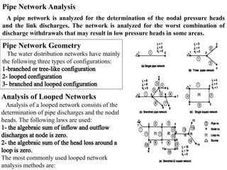
1. Pipe Network Analysis
A pipe network is analyzed for the determination of the nodal pressure heads
and the link discharges. The network is analyzed for the worst combination of
discharge withdrawals that may result in low pressure heads in some areas.
Pipe Network Geometry
The water distribution networks have mainly
the following three types of configurations:
Analysis of Looped Networks
Analysis of a looped network consists of the
determination of pipe discharges and the nodal
heads. The following laws are used:
The most commonly used looped network
analysis methods are:

2. 1- Hardy Cross Method
The following figure shows a relatively
simple network consisting of seven pipes,
two reservoirs, and one pump. The hydraulic
grade lines at A and F are assumed known;
these locations are termed fixed-grade
nodes. Outflow demands are present at
nodes C and D. Nodes C and D, along with
nodes B and E are called interior nodes or
junctions. Flow directions, even though not
initially known, are assumed to be in the
directions shown.
Representative piping network:
(a) assumed flow directions and
numbering scheme
(b) designated interior loops
(c) path between two fixed-grade nodes
1-1- Generalized Network Equations
Networks of piping, such as those shown in
the figure can be represented by the
following equations.
1. Continuity at the jth interior node:
± 𝑸𝒋 = 𝑸𝒆 -------(1)
in which the subscript j refers to the pipes
connected to a node, and Qe is the external.
Use the positive sign for flow into the junction,
and the negative sign for flow out of the
junction.

3. 2- Energy balance around an interior loop:
± 𝑾𝒊 − 𝑯𝒑𝒊 + ∆𝑯 = 𝟎 −−−−−−−(2)
𝑾𝒊 = 𝒌𝒊𝑸𝒊𝟐
= 𝑹𝒊𝑸𝒊𝟐
, 𝒌𝒊 = 𝑹𝒊 =
𝟖𝒇𝒊𝑳𝒊
𝝅𝟐𝒈𝑫𝒊𝟓
in which the subscript i pertains to the pipes that make up the loop. There will be a
relation for each of the loops. The plus and minus signs in Eq.2 follow the flow in the
element. If the flow is positive in the clockwise sense; otherwise, the minus sign is
employed.
∆𝑯: is the difference in magnitude of the two fixed-grade nodes in the path ordered in a
clockwise fashion across the imaginary pipe in the pseudoloop.
(HP)i is the head across a pump that could exist in the ith pipe element.
If F is the number of fixed-grade nodes, there will be (F -1) unique path equations.
Let P be the number of pipe elements in the network, J the number of interior nodes,
and L the number of interior loops. Then the following relation will hold if the network is
properly defined:
P = J + L + F – 1 -------(3)
In the figure above note that , J = 4, L = 2, F = 2, so that P = 4 + 2 + 2 -1 = 7

4. ∆𝑸𝒌 = −
± 𝑾𝒊−𝑯𝒑𝒊 +∆𝑯
𝑮𝒊
= −
± 𝒌𝒊𝑸𝒊 𝑸𝒊 −𝑯𝒑𝒊 +∆𝑯
𝟐 𝒌𝒊 𝑸𝒊 −
𝒅𝑯𝒑𝒊
𝒅𝑸
--------(6)
Where
𝒅𝑯𝒑𝒊
𝒅𝑸
= 𝒂𝟏 + 𝟐 𝒂𝟐 𝑸 or
𝒅𝑯𝒑𝒊
𝒅𝑸
= −
𝑷𝒐𝒘𝒆𝒓
𝜸𝑸𝟐 --------(7)
An approximate pump head-discharge representation is given by the polynomial
𝑯𝒑 = 𝒂𝒐 + 𝒂𝟏 𝑸 + 𝒂𝟐 𝑸𝟐 --------(4)
Or, 𝑯𝒑 =
𝑷𝒐𝒘𝒆𝒓
𝜸 𝑸
--------(5)
It is necessary for the algebraic sign of Q to be positive in the direction of
normal pump operation; otherwise, the pump curve will not be represented
properly and Eq.2 will be invalid. Furthermore, it is important that the discharge
Q through the pump remain within the limits of the data used to generate the
curve.
1-2- Linearization of System Energy Equations
Equation 2 is a general relation that can be applied to any path or closed loop in a
network. If it is applied to a closed loop, ∆𝑯 is set equal to zero, and if no pump exists in
the path or loop, (HP)i is equal to zero.
Simplifying the Eq.2 to a linear form using Taylor series and neglecting second power of
∆𝑄𝑘 yields

5. The Hardy Cross iterative solution is outlined in the following steps:
1. Assume an initial estimate of the flow distribution in the network that satisfies
continuity, Eq.1.
2. For each loop or path, evaluate ∆ 𝑸 with Eq.6
∆𝑸𝒌 =
− ± 𝑾𝒊−𝑯𝒑𝒊 −∆𝑯
𝑮𝒊
= −
± 𝒌𝒊𝑸𝒊 𝑸𝒊 −𝑯𝒑𝒊 +∆𝑯
𝟐 𝒌𝒊 𝑸𝒊 −
𝒅𝑯𝒑𝒊
𝒅𝑸
--------(6)
3. Update the flows in each pipe in all loops and paths, such that:
𝑸𝒊 𝒏𝒆𝒘 = 𝑸𝒊 𝒐𝒍𝒅 + ∆𝑸𝒌 --------(8)
The term ∆𝑸𝒌 is used, since a given pipe may belong to more than one loop; hence
the correction will be the sum of corrections from all loops to which the pipe is common.
4. Repeat steps 2 and 3 until a desired accuracy is attained. One possible
criterion to use is
𝑸𝒊−𝑸𝒐𝒊
𝑸𝒊
≤ 𝜺 in which 𝜺 is (0.001 < 𝜺 < 0.005)

6. Example 1: The pipe network of two loops as shown in Fig. 3.11 has to be
analyzed by the Hardy Cross method for pipe flows for given pipe lengths L and
pipe diameters D. The nodal inflow at node 1 and nodal outflow at node 3 are
shown in the figure. Assume a constant friction factor f = 0.02.
Solution
To apply continuity equation for initial pipe discharges, the discharges in pipes 1 and 5 equal to 0.1 m3/s
are assumed. The obtained discharges are
Q1 = 0.1 m3/s (flow from node 1 to node 2)
Q2 = 0.1 m3/s (flow from node 2 to node 3)
Q3 = 0.4 m3/s (flow from node 4 to node 3)
Q4 = 0.4 m3/s (flow from node 1 to node 4)
Q5 = 0.1 m3/s (flow from node 1 to node 3)
∆𝑸𝒌 = −
± 𝒌𝒊𝑸𝒊 𝑸𝒊 −𝑯𝒑𝒊 +∆𝑯
𝟐 𝒌𝒊 𝑸𝒊 −
𝒅𝑯𝒑𝒊
𝒅𝑸
∆𝑸𝟏 = −
𝒌𝟑𝑸𝟑 𝑸𝟑 +𝒌𝟒𝑸𝟒 𝑸𝟒 +𝒌𝟓𝑸𝟓 𝑸𝟓
𝟐𝒌𝟑 𝑸𝟑 +𝟐𝒌𝟒 𝑸𝟒 +𝟐𝒌𝟓 𝑸𝟓
∆𝑸𝟐 = −
𝒌𝟏𝑸𝟏 𝑸𝟏 +𝒌𝟐𝑸𝟐 𝑸𝟐 +𝒌𝟓𝑸𝟓 𝑸𝟓
𝟐𝒌𝟏 𝑸𝟏 +𝟐𝒌𝟐 𝟐 +𝟐𝒌𝟓 𝑸𝟓
𝑭𝒐𝒓 𝒄𝒐𝒎𝒎𝒐𝒏 𝒑𝒊𝒑𝒆 𝟓
𝑸𝟓 𝒏𝒆𝒘 = 𝑸𝟓 𝒐𝒍𝒅 ± ∆𝑸𝟏 ∓ ∆𝑸𝟐
There are four junctions (J = 4),
five pipes (P = 5), and (F= 0).
Hence the number of closed loops
is : L = P - J - F + 1
L = 5 - 4 - 0 + 1 = 2. The two loops
and the assumed flow directions
are as shown. Equation 6 is
applied to each loop as follows:

7. Example 2: For the piping system shown below, determine the flow distribution
and piezometric heads at the junctions using the Hardy Cross method of solution
Solution
∆𝑸𝒌 = −
± 𝒌𝒊𝑸𝒊 𝑸𝒊 −𝑯𝒑𝒊 +∆𝑯
𝟐 𝒌𝒊 𝑸𝒊 −
𝒅𝑯𝒑𝒊
𝒅𝑸
∆𝑸𝟏 = −
𝒌𝟒𝑸𝟒 𝑸𝟒 +𝒌𝟑𝑸𝟑 𝑸𝟑 +𝒌𝟐𝑸𝟐 𝑸𝟐 +𝒌𝟏𝑸𝟏 𝑸𝟏 +𝟐𝟎
𝟐𝒌𝟒 𝑸𝟒 +𝟐𝒌𝟑 𝑸𝟑 +𝟐𝒌𝟐 𝑸𝟐 +𝟐𝒌𝟏 𝑸𝟏
∆𝑸𝟐 = −
𝒌𝟐𝑸𝟐 𝑸𝟐 +𝒌𝟖𝑸𝟖 𝑸𝟖 +𝒌𝟕𝑸𝟕 𝑸𝟕 +𝒌𝟔𝑸𝟔 𝑸𝟔
𝟐𝒌𝟐 𝑸𝟐 +𝟐𝒌𝟖 𝑸𝟖 +𝟐𝒌𝟕 𝑸𝟕 +𝟐𝒌𝟔 𝑸𝟔
∆𝑸𝟑 = −
𝒌𝟑𝑸𝟑 𝑸𝟑 + 𝒌𝟓𝑸𝟓 𝑸𝟓 +𝒌𝟖𝑸𝟖 𝑸𝟖
𝟐𝒌𝟑 𝑸𝟑 + 𝟐𝒌𝟓 𝑸𝟓 +𝟐𝒌𝟖 𝑸𝟖
There are five junctions (J = 5), eight pipes (P =
8), and two fixed-grade nodes (F= 2). Hence the
number of closed loops is : L = P - J - F + 1
L = 8 - 5 - 2 + 1 = 2, plus one pseudo loop.
The three loops and the assumed flow directions
are as shown. Equation 6 is applied to each loop
as follows:
𝑸𝟐 𝒏𝒆𝒘 = 𝑸𝟐 𝒐𝒍𝒅 ± ∆𝑸𝟏 ∓ ∆𝑸𝟐
𝑸𝟑 𝒏𝒆𝒘 = 𝑸𝟑 𝒐𝒍𝒅 ± ∆𝑸𝟑 ∓ ∆𝑸𝟏
𝑭𝒐𝒓
𝒄𝒐𝒎𝒎𝒐𝒏
𝒑𝒊𝒑𝒆𝒔 𝟐, 𝟑, 𝟖 𝑸𝟖 𝒏𝒆𝒘 = 𝑸𝟖 𝒐𝒍𝒅 ± ∆𝑸𝟐 ∓ ∆𝑸𝟑

8. Example 3: Re solve example 2 considering a pump located at pipe 1 with
Hp = 250 – 0.4 Q – 0.1 Q 2
Solution
∆𝑸𝒌 = −
± 𝒌𝒊𝑸𝒊 𝑸𝒊 −𝑯𝒑𝒊 +∆𝑯
𝟐 𝒌𝒊 𝑸𝒊 −
𝒅𝑯𝒑𝒊
𝒅𝑸
∆𝑸𝟏 = −
𝒌𝟒𝑸𝟒 𝑸𝟒 +𝒌𝟑𝑸𝟑 𝑸𝟑 +𝒌𝟐𝑸𝟐 𝑸𝟐 +𝒌𝟏𝑸𝟏 𝑸𝟏 +𝑯𝒑 𝑸𝟏 +𝟐𝟎
𝟐𝒌𝟒 𝑸𝟒 +𝟐𝒌𝟑 𝑸𝟑 +𝟐𝒌𝟐 𝑸𝟐 +𝟐𝒌𝟏 𝑸𝟏 −(−𝟎.𝟒−𝟐∗𝟎.𝟏 𝑸𝟏 )
∆𝑸𝟐 = −
𝒌𝟐𝑸𝟐 𝑸𝟐 +𝒌𝟖𝑸𝟖 𝑸𝟖 +𝒌𝟕𝑸𝟕 𝑸𝟕 +𝒌𝟔𝑸𝟔 𝑸𝟔
𝟐𝒌𝟐 𝑸𝟐 +𝟐𝒌𝟖 𝑸𝟖 +𝟐𝒌𝟕 𝑸𝟕 +𝟐𝒌𝟔 𝑸𝟔
∆𝑸𝟑 = −
𝒌𝟑𝑸𝟑 𝑸𝟑 + 𝒌𝟓𝑸𝟓 𝑸𝟓 +𝒌𝟖𝑸𝟖 𝑸𝟖
𝟐𝒌𝟑 𝑸𝟑 + 𝟐𝒌𝟓 𝑸𝟓 +𝟐𝒌𝟖 𝑸𝟖
𝑸𝟐 𝒏𝒆𝒘 = 𝑸𝟐 𝒐𝒍𝒅 ± ∆𝑸𝟏 ∓ ∆𝑸𝟐
𝑸𝟑 𝒏𝒆𝒘 = 𝑸𝟑 𝒐𝒍𝒅 ± ∆𝑸𝟑 ∓ ∆𝑸𝟏
𝑸𝟖 𝒏𝒆𝒘 = 𝑸𝟖 𝒐𝒍𝒅 ± ∆𝑸𝟐 ∓ ∆𝑸𝟑
𝑭𝒐𝒓 𝒄𝒐𝒎𝒎𝒐𝒏 𝒑𝒊𝒑𝒆𝒔 𝟐, 𝟑, 𝟖

9. Example 4: Re solve example 2 considering a pump located at pipe 4 with
Hp = 250 – 0.4 Q – 0.1 Q 2
Solution
∆𝑸𝒌 = −
± 𝒌𝒊𝑸𝒊 𝑸𝒊 −𝑯𝒑𝒊 +∆𝑯
𝟐 𝒌𝒊 𝑸𝒊 −
𝒅𝑯𝒑𝒊
𝒅𝑸
∆𝑸𝟏 = −
𝒌𝟒𝑸𝟒 𝑸𝟒 +𝒌𝟑𝑸𝟑 𝑸𝟑 +𝒌𝟐𝑸𝟐 𝑸𝟐 +𝒌𝟏𝑸𝟏 𝑸𝟏 +𝑯𝒑 𝑸𝟒 +𝟐𝟎
𝟐𝒌𝟒 𝑸𝟒 +𝟐𝒌𝟑 𝑸𝟑 +𝟐𝒌𝟐 𝑸𝟐 +𝟐𝒌𝟏 𝑸𝟏 −(−𝟎.𝟒−𝟐∗𝟎.𝟏 𝑸𝟒 )
∆𝑸𝟐 = −
𝒌𝟐𝑸𝟐 𝑸𝟐 +𝒌𝟖𝑸𝟖 𝑸𝟖 +𝒌𝟕𝑸𝟕 𝑸𝟕 +𝒌𝟔𝑸𝟔 𝑸𝟔
𝟐𝒌𝟐 𝑸𝟐 +𝟐𝒌𝟖 𝑸𝟖 +𝟐𝒌𝟕 𝑸𝟕 +𝟐𝒌𝟔 𝑸𝟔
∆𝑸𝟑 = −
𝒌𝟑𝑸𝟑 𝑸𝟑 + 𝒌𝟓𝑸𝟓 𝑸𝟓 +𝒌𝟖𝑸𝟖 𝑸𝟖
𝟐𝒌𝟑 𝑸𝟑 + 𝟐𝒌𝟓 𝑸𝟓 +𝟐𝒌𝟖 𝑸𝟖
𝑸𝟐 𝒏𝒆𝒘 = 𝑸𝟐 𝒐𝒍𝒅 ± ∆𝑸𝟏 ∓ ∆𝑸𝟐
𝑸𝟑 𝒏𝒆𝒘 = 𝑸𝟑 𝒐𝒍𝒅 ± ∆𝑸𝟑 ∓ ∆𝑸𝟏
𝑸𝟖 𝒏𝒆𝒘 = 𝑸𝟖 𝒐𝒍𝒅 ± ∆𝑸𝟐 ∓ ∆𝑸𝟑
𝑭𝒐𝒓 𝒄𝒐𝒎𝒎𝒐𝒏 𝒑𝒊𝒑𝒆𝒔 𝟐, 𝟑, 𝟖

10. Example 5: Find the water flow distribution in the parallel system shown in figure
below. The pump Power is 799.68 Kw.
There are two junction (J = 1), four pipes (P = 4),
and two fixed-grade nodes (F= 2). Hence the
number of closed loops is : L = P - J - F + 1
L = 4 - 1 - 2 + 1 = 2 . There is one pseudo loop only
(F-1) only. The pseudo loop and the assumed flow
directions are as shown. Equation 6 is applied to
each loop as follows:
𝑸𝟐 𝒏𝒆𝒘 = 𝑸𝟐 𝒐𝒍𝒅 ± ∆𝑸𝟏 ∓ ∆𝑸𝟐
𝑭𝒐𝒓
𝒄𝒐𝒎𝒎𝒐𝒏
𝒑𝒊𝒑𝒆 𝟐 & 3
For pipe 1 𝒁𝟏 + 𝑯𝒑 − 𝒉𝒇𝟏 = 𝑯𝒋
𝟎 + 𝟐𝟕. 𝟎𝟒 − 𝟎. 𝟏𝟐𝟗𝟓 𝑸𝟏𝟐
= 𝑯𝒋 → 𝑯𝒋= 𝟐𝟕. 𝟎𝟒 − 𝟎. 𝟏𝟐𝟗𝟓 (𝟑)𝟐
= 25.874 m
Pipe L (m) D (mm) f ∑ K
1 100 1200 0.015 2
2 1000 1000 0.020 3
3 1500 500 0.018 2
4 800 750 0.021 4
∆𝑸𝒌 = −
± 𝒌𝒊𝑸𝒊 𝑸𝒊 −𝑯𝒑𝒊 +∆𝑯
𝟐 𝒌𝒊 𝑸𝒊 −
𝒅𝑯𝒑𝒊
𝒅𝑸
∆𝑸𝟏 = −
𝒌𝟐𝑸𝟐 𝑸𝟐 +𝒌𝟏𝑸𝟏 𝑸𝟏 +𝑯𝒑(𝑸𝟏)−𝟐𝟎
𝟐𝒌𝟐 𝑸𝟐 +𝟐𝒌𝟏 𝑸𝟏 +
𝟕𝟗𝟗.𝟔𝟖
𝟗.𝟖 𝒙 𝑸𝟏𝟐
∆𝑸𝟐 = −
𝒌𝟐𝑸𝟐 𝑸𝟐 +𝒌𝟑𝑸𝟑 𝑸𝟑
𝟐𝒌𝟐 𝑸𝟐 +𝟐𝒌𝟑 𝑸𝟑
∆𝑸𝟑 = −
𝒌𝟑𝑸𝟑 𝑸𝟑 + 𝒌𝟒𝑸𝟒 𝑸𝟒
𝟐𝒌𝟑 𝑸𝟑 + 𝟐𝒌𝟒 𝑸𝟒
𝑸𝟑 𝒏𝒆𝒘 = 𝑸𝟑 𝒐𝒍𝒅 ± ∆𝑸𝟐 ∓ ∆𝑸𝟑
[I]
[II]
[III]

11. Example 6: For the piping system shown below, determine the flow distribution
and piezometric heads at the junction J using the Hardy Cross method of solution
Solution
∆𝑸𝒌 = −
± 𝒌𝒊𝑸𝒊 𝑸𝒊 −𝑯𝒑𝒊 +∆𝑯
𝟐 𝒌𝒊 𝑸𝒊 −
𝒅𝑯𝒑𝒊
𝒅𝑸
∆𝑸𝟏 = −
𝒌𝟐𝑸𝟐 𝑸𝟐 +𝒌𝟏𝑸𝟏 𝑸𝟏 +𝟒𝟎
𝟐𝒌𝟐 𝑸𝟐 +𝟐𝒌𝟏 𝑸𝟏
∆𝑸𝟐 = −
𝒌𝟑𝑸𝟑 𝑸𝟑 +𝒌𝟐𝑸𝟐 𝑸𝟐 +𝟏𝟓
𝟐𝒌𝟐 𝑸𝟐 +𝟐𝒌𝟑 𝑸𝟑
There are one junction (J = 1), three pipes (P = 3),
and three fixed-grade nodes (F= 3). Hence the
number of closed loops is : L = P - J - F + 1
L = 3 - 1 - 3 + 1 = 0 . There are two pseudo loop
(F-1) only. The two pseudo loop and the assumed
flow directions are as shown. Equation 6 is
applied to each loop as follows:
𝑸𝟐 𝒏𝒆𝒘 = 𝑸𝟐 𝒐𝒍𝒅 ± ∆𝑸𝟏 ∓ ∆𝑸𝟐
𝑭𝒐𝒓 𝒄𝒐𝒎𝒎𝒐𝒏 𝒑𝒊𝒑𝒆 𝟐
𝑲𝒇
f
D (m)
L (m)
Pipe
0
0.01
0.3
1500
1
0
0.01
0.3
1500
2
0
0.01
0.3
1500
3
From Res. A to Junction j
→ 𝒉𝒇𝟏 = 𝑲𝟏 𝑸𝟏𝟐 → 𝒉𝒇𝟏 = 𝟓𝟏𝟎. 𝟎𝟒𝟐 𝑸𝟏𝟐 = 70 – hj
→ 𝒉𝒋 = 𝟕𝟎 − 𝟓𝟏𝟎. 𝟎𝟒𝟐 𝑸𝟏𝟐 = 𝟕𝟎 − 𝟓𝟏𝟎. 𝟎𝟒𝟐 𝟎. 𝟐𝟔𝟖𝟕 𝟐 = 𝟑𝟑. 𝟏𝟕𝟓 𝒎
[1]
[2]

12. Example 7: For the piping system shown below, determine the flow distribution
and piezometric heads at the junction J using the Hardy Cross method of solution
Solution
∆𝑸𝒌 = −
± 𝒌𝒊𝑸𝒊 𝑸𝒊 −𝑯𝒑𝒊 +∆𝑯
𝟐 𝒌𝒊 𝑸𝒊 −
𝒅𝑯𝒑𝒊
𝒅𝑸
∆𝑸𝟏 = −
𝒌𝟐𝑸𝟐 𝑸𝟐 +𝒌𝟏𝑸𝟏 𝑸𝟏 −𝟐𝟎
𝟐𝒌𝟐 𝑸𝟐 +𝟐𝒌𝟏 𝑸𝟏 +
𝟐𝟎
𝟗.𝟖 𝒙 𝑸𝟏𝟐
∆𝑸𝟐 = −
𝒌𝟑𝑸𝟑 𝑸𝟑 +𝒌𝟐𝑸𝟐 𝑸𝟐 +𝟏𝟓
𝟐𝒌𝟐 𝑸𝟐 +𝟐𝒌𝟑 𝑸𝟑
There are one junction (J = 1), three pipes (P = 3),
and three fixed-grade nodes (F= 3). Hence the
number of closed loops is : L = P - J - F + 1
L = 3 - 1 - 3 + 1 = 0 . There are two pseudo loop
(F-1) only. The two pseudo loop and the assumed
flow directions are as shown. Equation 6 is
applied to each loop as follows:
𝑸𝟐 𝒏𝒆𝒘 = 𝑸𝟐 𝒐𝒍𝒅 ± ∆𝑸𝟏 ∓ ∆𝑸𝟐
𝑭𝒐𝒓 𝒄𝒐𝒎𝒎𝒐𝒏 𝒑𝒊𝒑𝒆 𝟐
𝑲𝒇
f
D (m)
L (m)
Pipe
2
0.02
0.15
50
1
1
0.015
0.10
100
2
1
0.025
0.10
300
3
For pipe 1 𝒁𝟏+ 𝑯𝒑= 𝒉𝒇𝟏 + 𝑯𝒋
𝟏𝟎 +
𝟐𝟎
𝟗.𝟖 𝑸𝟏
= 𝟏𝟒𝟐𝟎 𝑸𝟏𝟐 + 𝑯𝒋 → 𝑯𝒋= 𝟏𝟎 +
𝟐𝟎
𝟗.𝟖 𝑸𝟏
− 𝟏𝟒𝟐𝟎 𝑸𝟏𝟐
=𝟏𝟎 +
𝟐𝟎
𝟗.𝟖 𝒙 𝟎.𝟎𝟓𝟑𝟔
− 𝟏𝟒𝟐𝟎 (𝟎. 𝟎𝟓𝟑𝟔)𝟐
= 43.995 m
[1]
[2]

13. Example 8: Determine the flow distribution of water in the system shown in Fig.
Assume constant friction factors, with f 0.02.The head-discharge relation for the
pump is HP = 60 -10Q2 .
Solution
∆𝑸𝒌 = −
± 𝒌𝒊𝑸𝒊 𝑸𝒊 −𝑯𝒑𝒊 +∆𝑯
𝟐 𝒌𝒊 𝑸𝒊 −
𝒅𝑯𝒑𝒊
𝒅𝑸
∆𝑸𝟏 = −
𝒌𝟒𝑸𝟒 𝑸𝟒 +𝒌𝟐𝑸𝟐 𝑸𝟐 +𝒌𝟏𝑸𝟏 𝑸𝟏 +𝑯𝒑−𝟓𝟎
𝟐𝒌𝟒𝑸𝟒 𝑸𝟒 +𝟐𝒌𝟐 𝑸𝟐 +𝟐𝒌𝟏 𝑸𝟏 −(−𝟐𝟎 𝑸𝟏 )
∆𝑸𝟐 = −
𝒌𝟓𝑸𝟓 𝑸𝟓 +𝒌𝟒𝑸𝟒 𝑸𝟒 +𝟐
𝟐𝒌𝟓 𝑸𝟓 + 𝟐𝒌𝟒 𝑸𝟒
∆𝑸𝟑 = −
𝒌𝟐𝑸𝟐 𝑸𝟐 + 𝒌𝟑𝑸𝟑 𝑸𝟑
𝟐𝒌𝟐 𝑸𝟐 + 𝟐𝒌𝟑 𝑸𝟑
junctions (J = 2), pipes (P = 5), and fixed-grade
nodes (F= 3). Hence the number of closed loops is :
L = P - J - F + 1
L = 5 - 2 - 3 + 1 = 1 . There are two pseudo loop (F-
1) only. The two pseudo loop and the assumed flow
directions are as shown. Equation 6 is applied to
each loop as follows:
𝑸𝟐 𝒏𝒆𝒘 = 𝑸𝟐 𝒐𝒍𝒅 ± ∆𝑸𝟏 ∓ ∆𝑸𝟑
𝑭𝒐𝒓 𝒄𝒐𝒎𝒎𝒐𝒏 𝒑𝒊𝒑𝒆 𝟐
𝑸𝟒 𝒏𝒆𝒘 = 𝑸𝟒 𝒐𝒍𝒅 ± ∆𝑸𝟏 ∓ ∆𝑸𝟐
[1]
[2]
[3]