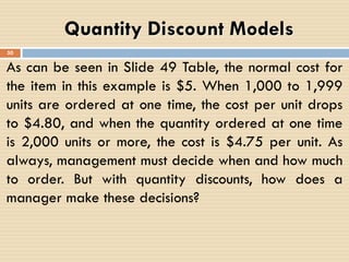
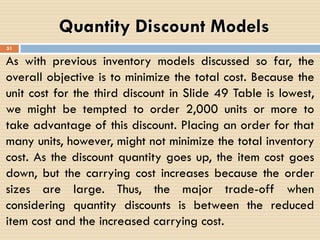
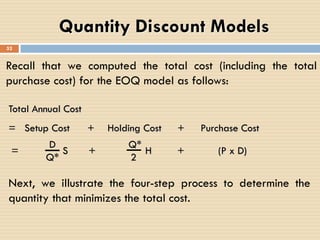
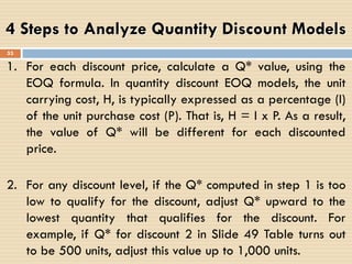
Download as PDF, PPTX


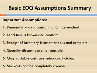
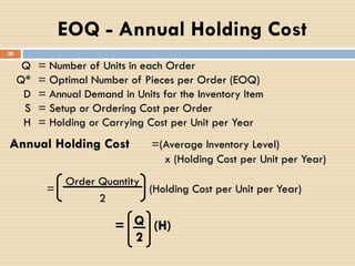
![[Refer to Graph in Slide 19]
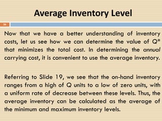
With these assumptions, inventory usage has a
sawtooth shape. In the graph, Q represents the
amount that is ordered. If this amount is 500 units, all
500 units arrive at one time when an order is
received. Thus, the inventory level jumps from 0 to 500
units. In general, the inventory level increases from 0
to Q units when an order arrives.
20
Inventory Usage Over Time](https://image.slidesharecdn.com/basiceoqmodel-quantitydiscount-economiclotsize-160803220037/85/Basic-EOQ-Model-Quantity-Discount-Economic-Lot-Size-20-320.jpg)
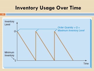
![[Refer to Graph in Slide 19]
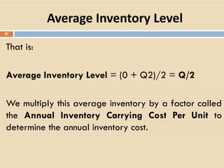
Because demand is constant over time, inventory drops
at a uniform rate over time. Another order is placed
such that when the inventory level reaches 0, the new
order is received and the inventory level again jumps
to Q units, represented by the vertical lines. This
process continues indefinitely over time.
21
Inventory Usage Over Time](https://image.slidesharecdn.com/basiceoqmodel-quantitydiscount-economiclotsize-160803220037/85/Basic-EOQ-Model-Quantity-Discount-Economic-Lot-Size-21-320.jpg)
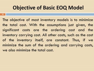
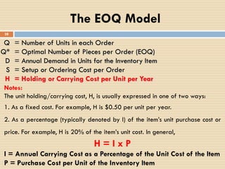
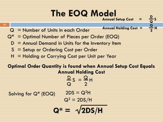
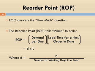
![24
Objective of Basic EOQ Model
[Refer to Graph in Slide 23]
To help visualize this, Slide 23 graphs total cost as a
function of the order quantity, Q. As the value of Q
increases, the total number of orders placed per year
decreases. Hence, the total ordering cost decreases.
However, as the value of Q increases, the carrying
cost increases because the firm has to maintain larger
average inventories.](https://image.slidesharecdn.com/basiceoqmodel-quantitydiscount-economiclotsize-160803220037/85/Basic-EOQ-Model-Quantity-Discount-Economic-Lot-Size-24-320.jpg)
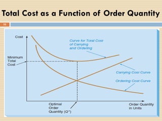
![25
Objective of Basic EOQ Model
[Refer to Graph in Slide 23]
The optimal order size, Q*, is the quantity that
minimizes the total cost. Note in Slide 23 that Q*
occurs at the point where the ordering cost curve and
the carrying cost curve intersect. This is not by chance.
With this particular type of cost function, the optimal
quantity always occurs at a point where the ordering
cost is equal to the carrying cost.](https://image.slidesharecdn.com/basiceoqmodel-quantitydiscount-economiclotsize-160803220037/85/Basic-EOQ-Model-Quantity-Discount-Economic-Lot-Size-25-320.jpg)
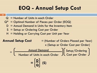
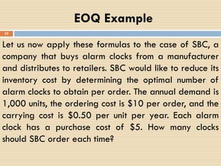
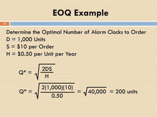
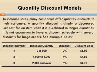
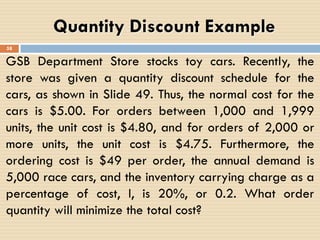
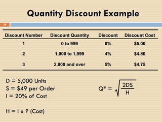
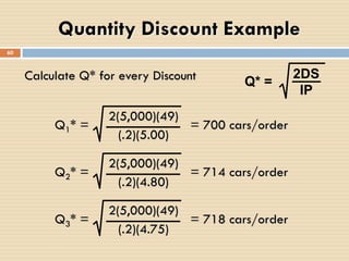
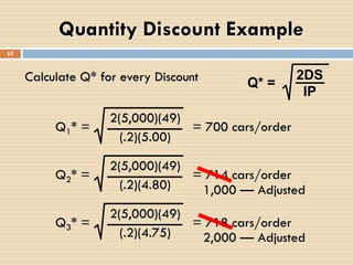
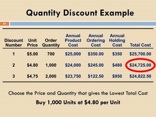
![In the GSB Department Store example, observe that
the Q* values for discounts 2 and 3 are too low to be
eligible for the discounted prices (Slide 49 Table).
They are, therefore, adjusted upward to 1,000 and
2,000, respectively.
With these adjusted Q* values, we find that the lowest
total cost of $24,725 results when we use an order
quantity of 1,000 units [See Slide 61 and Slide 62].
Quantity Discount Example
61](https://image.slidesharecdn.com/basiceoqmodel-quantitydiscount-economiclotsize-160803220037/85/Basic-EOQ-Model-Quantity-Discount-Economic-Lot-Size-61-320.jpg)


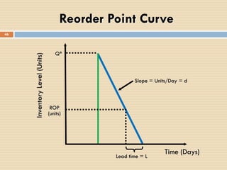
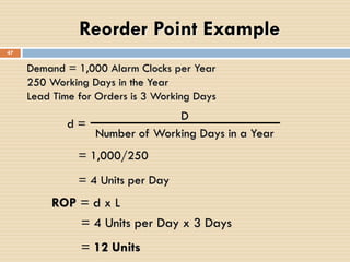
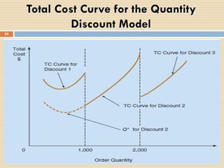
This document discusses inventory models, including the basic economic order quantity (EOQ) model and quantity discounts. It begins by defining inventory and explaining the importance of inventory control. It then covers the basic EOQ model assumptions and formulas for calculating optimal order quantity, expected number of orders per year, time between orders, total cost, and average inventory value. The document also discusses using a reorder point and provides an example calculation. Finally, it introduces quantity discount models, where purchasing larger quantities results in decreased unit costs.


