SlideShare a Scribd company logo
1 of 37
Prof. David R. Jackson
Dept. of ECE
Notes 8
ECE 5317-6351
Microwave Engineering
Fall 2019
Waveguiding Structures
Part 3: Parallel Plates
1
, ,
  
x
z
y
d
w
Adapted from notes by
Prof. Jeffery T. Williams
2
2
2
2
z z
x c z
c
z z
y c z
c
z z
x z
c
z z
y z
c
E H
j
H k
k y x
E H
j
H k
k x y
E H
j
E k
k x y
E H
j
E k
k y x




 
 
  
 
 
 
 

 
 
 
 
 
 

  
 
 
 
 
 
 
 
 
 
Summary
2 2
c
k  

2 2
c z
k k k
 
Field Equations (from Notes 6)
This table of fields will be useful
to us in the present discussion.
2
(kc is always real)
(k can be complex)
z
jk z
e
0
1
(1 tan )
(1 tan )
c
c c
c
c
c
c d
r
j
j j
j
j
j
j

 


 

 



 
  
 
 
  
 
 

 

 
 

 

 
 
Assumption:
Parallel-Plate Waveguiding Structure
 Both plates assumed PEC
 w >> d
0
x

 

The parallel-plate structure is a good approximate model for a wide microstrip line.
3
(neglect edge effects)
,
w
h
, ,
  
c j

 

 
, ,
  
x
z
y
d
w
PEC
4
TEM Solution Process
A) Solve Laplace’s equation subject to appropriate B.C.s.:
B) Find the transverse electric field:
C) Find the total electric field:
D) Find the magnetic field:
 
2
, 0
x y
  
 
1
ˆ ;
H z E z

    propagation
   
, ,
t
e x y x y
 
   
, , , ,
z
jk z
t z
E x y z e x y e k k
 
Note: The only frequency dependence is in the wavenumber kz = k.
2 conductors  1 TEM mode
To solve for TEM mode:
 
2
, 0
x y
  
Boundary conditions:
0
( ,0) 0 ; ( , )
x x d V
   
2 2
2
2 2
0
x y
 
 
     
 
 
 
TEM Mode
z c
k j k k jk
     
     
k
k






5
0
0
x w
y d
 
 
, ,
  
x
z
y
d
w
PEC
where
( , )
x y A By
  
0
ˆ
( , , ) ( , ) jkz jkz
t
V
E x y z e x y e y e
d
  
0
A 
2
2
0
y
 


    0
,0 0 & ,
x x d V
   
  0
ˆ ˆ
,
t
V
e x y y y
y d

      

TEM Mode (cont.)
6
0
V
B
d

0
( , )
V
x y y
d
 
Hence
We then have
Recall
  0
ˆ
, , jkz
V
H x y z x e
d

  
1
ˆ
( )
H z E

  
0
ˆ
( , , ) jkz
V
E x y z y e
d
 
TEM Mode (cont.)
7
c




c j

 

 
Fields for +z mode: E
H
x
y
0
V
, ,
  
, ,
  
x
z
y
d
w
PEC
TEM Mode (cont.)
8
We can view the TEM mode in a parallel-plate waveguiding structure
as a rectangular “slice” of a plane wave.
The PEC and PMC walls do not disturb the fields of the plane wave.
ˆ 0
n E
 
PEC : ˆ 0
n H
 
PMC :
PEC
PEC
PMC
PMC , ,
  
x
E
H
y
PEC: Perfect Electric Conductor PMC: Perfect Magnetic Conductor
Assume a wave propagating the
in + z direction henceforth.
Time-ave power flow in + z direction:
 
*
2
0 2
* 2
0 0
2 2
0 2 *
1
ˆ
Re ( )
2
1
ˆ ˆ
Re
2
1 1 1
Re
2
s
w d
k z
k z
P E H z dS
V
z z e dydx
d
V wd e
d







 
  
 
 
 
 
 
  
 
 
 
 
 
 
 
    
   


2 2
0 *
1 1
Re
2
k z
w
P V e
d 

 
 
 
    
   
TEM Mode (cont.)
9
 
0
0
ˆ
( , , )
ˆ
, ,
jkz
jkz
V
E x y z y e
d
V
H x y z x e
d



 

, ,
  
x
z
y
d
w
PEC
Transmission line voltage
 
0
0
ˆ
( )
( )
d
jkz
V z E y dy
V z V e
 
 

Transmission line current
 
0
top
0 0
0
( ) , ,
( )
w w
sz x
jk
I
z
I z J dx H x d z dx
V
I z we
d


 
 
  Characteristic Impedance
0
0
0
jkz
jkz
V e
Z
I e



0
d
Z
w


TEM Mode (cont.)
10
top
ˆ ( )
s sz x
J n H J H
   
Note : On PEC on top plate
, ,
  
x
z
y
d
w
I


V
PEC
I
c




c j

 

 
Time-ave power flow in +z direction:  
*
*
2
0
0
2 2
0 *
1
Re
2
1
Re
2
1 1
Re
2
k z
k z
P VI
V
V w e
d
w
P V e
d






 

 
 
 
  
 
 
 
 
 
 
    
   
Recall that we found from
the fields that:
2 2
0 *
1 1
Re
2
k z
w
P V e
d 

 
 
 
    
   
Same
TEM Mode (cont.)
(calculated using the voltage and current)
This is expected, since a TEM mode is a
transmission-line type of mode, which is
described by voltage and current.
11
Recall:
where
   
2 2
2
2 2
, ,
z c z
e x y k e x y
x y
 
 
  
 
 
 
( , , ) ( , ) z
jk z
z z
E x y z e x y e

TMz Modes (Hz = 0)
12
   
2 2
, ,
t z c z
e x y k e x y
  
eigenvalue problem
2 2
c z
k k k
 
   
2
2
2 z c z
d
e y k e y
dy
 
(Assume no x variation)
so
Note:
Solving the eigenvalue problem
(using appropriate boundary conditions)
will tell us what the eigenvalue kc is.
, ,
  
x
z
y
d
w
PEC
  sin( ) cos( )
@ 0 0
@ 1,2,...
z c
c c
c
e y A k y B k y
y B
y d k d n n
n
k
d


 
  
     
ApplyB.C.'s :
subject to B.C.’s Ez = 0 @ y = 0, d
13
   
2
2
2 z c z
d
e y k e y
dy
 
Solving the above equation:
TMz Modes (cont.)
, ,
  
x
z
y
d
w
PEC
  sin 1,2,...
z
n
e y A y n
d

 
 
 
 
 
, sin z
jk z
z n
n
E y z A y e
d
 
 
   
 
For a wave propagating in the +z direction:
2 2
2 2
cos
cos
z
z
jk z
c z c
x n
c c
jk z
z z z
y n
c c
j E j n n
H A y e
k y k d d
jk E jk n n
E A y e
k y k d d
   
 


    
     
    
    
       
    
 
1/2
2
1/2
2 2 2
z c
n
k k k k
d

 
 
   
 
 
 
 
 
2 2
c
k  

TMz Modes (cont.)
14
No x variation TMz mode
0 0 0
x y z
E H H
  
sin z
jk z
z n
n
E A y e
d
 
 
  
 
Summary
1/2
2
2
2 2
cos
cos
0
; 1,2,...
z
z
jk z
z
y n
c
jk z
c
x n
c
x y z
c
z
c
jk n
E A y e
k d
j n
H A y e
k d
E H H
n
k n
d
n
k k
d
k

 


 


 
   
 
 
  
 
  
 
 
 
 
 
 
 
 
 

Each value of n corresponds to a unique TMz
field solution or “mode” in the waveguide.
 TMn mode
Note:
0
0
TM TEM
z
n k k
  
 
15
TMz Modes (cont.)
The TEM mode can be thought of as a TM0 mode.
, ,
  
x
z
y
d
w
PEC
 
2 1/2
2
2
1/2
2 2
c
k
z
c
n
k k
d
k k

 
 
 
 
   
 
 
 
 
 
0,1,2,...
n 
2 2
2
2
2 2 2
2
z
z c z c
c
j z
c
k z
k k k k j k k j
e
k k k k
e 
 
 
         





propagating mode
For For
Fields decay exponentially
 “evanescent” mode
Lossless Case
c
  
 
 
2 2
k  
 real
16
TMz Modes (cont.)
, ,
  
x
z
y
d
w
PEC
Cutoff frequency (for lossless case)
fc  cutoff frequency
@ c
f f
 c c
n
k k
d

 
  
1
2
c cn
n
f f
d 
  cutoff frequency for TMn mode
17
c
  
 
TMz Modes (cont.)
Note: For a lossy waveguide, there is no sharp definition of cutoff frequency.
This is the frequency that defines the border between evanescence and propagation.
Time average power flow in z direction (lossless case):
 
*
0 0
*
0 0
2 2 2
2
0
1
ˆ
Re
2
1
Re
2
Re{ } cos
2
w d
TMn
w d
y x
d
z
z n
c
P E H z dydx
E H dydx
n
k A w y dy e
k d

  
 
  
 
 
 
   
 
 
  
 



2 2
2
Re{ }
2 2
1,2,...
z
TMn z n
c
d
P k A w e
k
n

 
 
  
 

18
c
  
 
TMz Modes (cont.)
cos
cos
z
z
jk z
z
y n
c
jk z
c
x n
c
jk n
E A y e
k d
j n
H A y e
k d

 


 
   
 
 
  
 
z c
z c
k
k i
f f
f f


is realfor
is maginary for
, ,
  
x
z
y
d
w
PEC
Recall:
where
   
2 2
2
2 2
, ,
z c z
h x y k h x y
x y
 
 
  
 
 
 
( , , ) ( , ) z
jk z
z z
H x y z h x y e

TEz Modes (Ez = 0)
19
   
2 2
, ,
t z c z
h x y k h x y
  
eigenvalue problem
2 2
c z
k k k
 
   
2
2
2 z c z
d
h y k h y
dy
 
(Assume no x variation)
so
Note:
Solving the eigenvalue problem
(using appropriate boundary conditions)
will tell us what the eigenvalue kc is.
, ,
  
x
z
y
d
w
PEC
subject to B.C.’s Ex = 0 @ y=0, d
1 y
z
x
c
H
H
E
j y z


 

 
 
 
 
TEz Modes (cont.)
ˆ 0, 0
t
H n E
  
PEC:
20
0
z
h
y



Solving the above equation:
   
2
2
2 z c z
d
h y k h y
dy
 
sin( ) cos( )
cos( ) sin( )
@ 0 0
@ , 1,2,3,...
z c
c c
c
c
z c c
c
n
h A k y B k y
h k A k y k B k y
y A
n
d
d k d n k
y 

 
 
  
  
   
ApplyB.C.'s:
, ,
  
x
z
y
d
w
PEC
  cos 1,2,3,...
z n
n
h y B y n
d

 
 
 
 
2 2
2 2
sin
sin
z
z
jk z
z
x n
c c
jk z
z z z
y n
c c
j H j n n
E B y e
k y k d d
jk H jk n n
H B y e
k y k d d
   
 


     
     
    
    
      
    
 
1/2
2 2
1/2
2
2
z c
k k k
n
k
d

 
 
 
 
 
 
 
 
 
2 2
c
k  

TEz Modes (cont.)
21
 
, cos z
jk z
z n
n
H y z B y e
d
 
 
  
 
0 0 0
x y z
H E E
  
For a wave propagating in the +z direction:
No x variation TEz mode
Summary
cos z
jk z
z n
n
H B y e
d
 
 
  
 
Cutoff frequency
1
2
c cn
n
f f
d 
 
   
 
Each value of n corresponds to a
unique TEz field solution or “mode.”
1/2
2
2
2 2
sin
sin
0
; 1,2,...
z
z
jk z
x n
c
jk z
z
y n
c
x y z
c
z
c
j n
E B y e
k d
jk n
H B y e
k d
H E E
n
k n
d
n
k k
d
k
 



 


 
  
 
 
  
 
  
 
 
 
 
 
 
 
 
 

22
TEz Modes (cont.)
 TEn mode
Note: There is no TE0 mode
(This mode would be a plane wave having Ex and Hy, but
would not be supported by this system. This mode would
require PMC on top and bottom, and PEC on the sides.)
, ,
  
x
z
y
d
w
PEC
 
*
0 0
*
0 0
2 2 2
2
0
1
ˆ
Re
2
1
Re
2
Re{ } sin
2
w d
TEn
w d
x y
d
z
z n
c
P E H z dydx
E H dydx
n
k B w y dy e
k d

 


 
  
 
 
 
  
 
 
  
 



   
2 2
2
Re
4
z
TEn z n
c
P k B wd e
k


 

Power in TEz Mode
Time average power flow in z direction (lossless case):
23
c
  
 
sin
sin
z
z
jk z
x n
c
jk z
z
y n
c
j n
E B y e
k d
jk n
H B y e
k d
 



 
  
 
 
  
 
, ,
  
x
z
y
d
w
PEC
z c
z c
k
k i
f f
f f


is realfor
is maginary for
For all the modes of a parallel-plate waveguiding structure, we have
1
2
cn
n
f
d 
 
  
 
 
The mode with lowest cutoff frequency is called the
“dominant” mode of the waveguide.
Mode Chart
24
c
  
 
Important conclusion: If we want to use the structure as a
transmission line, we need to operate in the region f < fc1.
TEM TM1 TM2 TM3
Single
mode
prop.
3
modes
prop
5
mode
prop.
0
….
TE3
TE2
TE1
f
1
c
f 2
c
f 3
c
f
Field Plots
25
TEM
TM1
TE1
(from Pozar book)
x
x
x
y
y
y
Plane Wave Interpretation
26
sin
cos
cos
z
z
z
jk z
z n
jk z
z
y n
c
jk z
c
x n
c
n
E A y e
d
jk n
E A y e
k d
j n
H A y e
k d


 



 
  
 
 
   
 
 
  
 
TMz waveguide mode propagating in +z direction:
 
 
 
sin
cos
cos
z
z
z
jk z
z n y
jk z
z
y n y
c
jk z
c
x n y
c
E A k y e
jk
E A k y e
k
j
H A k y e
k





 

c
n
k
d


Re-label this as ky
 
 
 
1
2
2
2
y y
z z
y y
z z
y y
z z
jk y jk y
jk z jk z
z n
jk y jk y
jk z jk z
z
y n
c
jk y jk y
jk z jk z
c
x n
c
E A e e e e
j
jk
E A e e e e
k
j
H A e e e e
k

 
 
 
 
 
 
 
  
 
 
  
 
       
1 1
cos sin
2 2
jx jx jx jx
x e e x e e
j
 
   
Plane Wave Interpretation (cont.)
27
The TMz waveguide mode is a sum of two plane waves*:
 
 
 
1
2
2
2
y y
z z
y y
z z
y y
z z
jk y jk y
jk z jk z
z n
jk y jk y
jk z jk z
z
y n
c
jk y jk y
jk z jk z
c
x n
c
E A e e e e
j
jk
E A e e e e
k
j
H A e e e e
k

 
 
 
 
 
 
 
  
 
 
  
 
cos
z
k k 

 
z
y


E
E
H H
z
TM Side view
, ,
  
x
z
y
d
w
PEC
*We can also think of one a single plane wave bouncing up and down.
28
The TEz waveguide mode is a sum of two plane waves*:
 
 
 
 
 
1
2
2
2
y y
z z
y y
z z
y y
z z
jk y jk y
jk z jk z
z n
jk y jk y
jk z jk z
x n
c
jk y jk y
jk z jk z
z
y n
c
H B e e e e
j
E B e e e e
j k
jk
H B e e e e
j k

 
 
 
 
 
 
 
 
 
 
  
  
Plane Wave Interpretation (cont.)
 
cos
z
k k 

z
y
z
TE
H
H
E
E


Side view
, ,
  
x
z
y
d
w
PEC
*We can also think of one a single plane wave bouncing up and down.
Conductor Attenuation on Parallel Plates
 
*
0
0 0
2
0
2
0 0
2
0
1
ˆ
Re
2
1
ˆ ˆ
Re
2
1 1
2
w d
w d
P E H z dydx
V
z z dydx
d
w
V
d


 
  
 
 
 
 
 
  
 
 
 
 
 
 
 
   
  


0
0
ˆ
ˆ
jkz
jkz
V
E y e
d
V
H x e
d



 
 
top
0
ˆ
ˆ
s
jkz
J y H
V
z e
d


  

bot 0
ˆ ˆ jkz
s
V
J y H z e
d


   
On the top plate:
On the bottom plate:
29
Assume no dielectric
loss for the calculation
of conductor
attenuation.
TEM Mode
, Real
k  
0
(0)
2
l
c
P
P
 
x
z
y
d
w
m

c
  
  m

2 2
top bot
0 0
0 0
(0)
2
w w
s
l s s
z z
R
P J dx J dx
 
 
 
 
 
 
2
0
0
w
s
V
R dx
d

 
2
0
2
( )
s
V
R w
d


2
0 2
2
0
0
( )
(0)
2 1
2
2
s
l
c
w
R V
d
P
P w
V
d



 
 
 
 
 
 
   
   
s
c
R
d



(equal contributions from both plates)
The final result is then
30
Conductor Attenuation on Parallel Plates (cont.)
We then have:
1 2
2 2
1 1
0 0
1 1
(0)
2 2
l s s s s
C C
z z
P R J d R J d
 
 
 
31
Let’s try the same calculation using the Wheeler incremental inductance rule.
cond 0
0
2
s
c
R Z
Z


  
  

 
0
d
Z
w

 
  
 
From previous
calculations:
top bot
c c c
  
 
0 0
Z dZ
d


 
( d
  for eitherplate)
since
Conductor Attenuation on Parallel Plates (cont.)
,
 
, Real
k  
w
d
In this formula, (for a given conductor) is the
distance by which the conducting boundary is
receded away from the field region.
We apply the formula for each conductor and then add the results:
s
c
R
d



32
cond 0
0
2
s
c
R Z
Z


  
  

 
0
d
Z
w

 
  
 
0 0
Z dZ
d


 
top
0 0
2 2 2
2
s s s s
c
R R R R
d
d
Z d w wZ d
w
w
 
 

    
   
   
  
 
 
 
 
bot
0 0
2 2 2
2
s s s s
c
R R R R
d
d
Z d w wZ d
w
w
 
 

    
   
   
  
 
 
 
 
Hence, we have:
Conductor Attenuation on Parallel Plates (cont.)
,
 
, Real
k  
w
d
33
Surface Roughness
Conductor attenuation will increase due to surface roughness effects.
①
②
③
④
200 m
Surfaces 3 and 4 are rough.
Stripline
34
Surface Roughness (cont.)
We can use an effective conductivity to account for surface roughness.
 
7
3.0 10 S/m
  
Pure copper
 
7
5.8 10 S/m
  
Practical copper
Example:
35
Surface Roughness (cont.)
https://www.microwaves101.com/encyclopedias/surface-roughness
2
1
rough
2
1 tan 1.4 a
R
K
 

 
 
   
 
 
 
 
Hammerstad and Jensen formula
E. Hammerstad and O. Jensen,
“Accurate models for microstrip
computer-aided design,” in
Microwave Symp. Digest, IEEE
MTT-S International, 1980, vol. 1,
no. 12, pp. 407–409.
Attenuation factor Krough vs. surface roughness
Attenuation
factor
Ratio of roughness Ra to skin depth 
This is a factor that gives the increase in the attenuation constant .
Ra = height of surface roughness
36
Surface Roughness (cont.)
r
r
Ar
rbase
…
…
Ar: Hemispheroid height
rbase: Hemispheroid radius
r: Period
X. Guo, D. R. Jackson, M. Y. Koledintseva, S. Hinaga, J. L. Drewniak, and J. Chen, “An Analysis
of Conductor Surface Roughness Effects on Signal Propagation for Stripline Interconnects,” IEEE
Trans. Electromagnetic Compatibility, Vol. 56, No. 3, pp. 707–714, June 2014.
base / 1/ 3
r
r  
Results for TM/TE Modes (above cutoff): (derivation omitted)
TMn modes of PPW:
TM 2
, 0
s
cn
kR
n
d


 
TEn modes of PPW:
2
TE 2
, 0
c s
cn
k R
n
k d


 
37
Note: Below cutoff, we usually do not worry about conductor loss.
Conductor Attenuation on Parallel Plates (cont.)
Waveguide Modes
x
z
y
d
w
m

c
  
  m


More Related Content

Similar to Waveguiding Structures Part 3 (Parallel Plates).pptx

Rectangular waveguides
Rectangular waveguidesRectangular waveguides
Rectangular waveguideskhan yaseen
 
Transmission Lines Part 1 (TL Theory).pptx
Transmission Lines Part 1 (TL Theory).pptxTransmission Lines Part 1 (TL Theory).pptx
Transmission Lines Part 1 (TL Theory).pptxRituparna Mitra
 
Waveguiding Structures Part 2 (Attenuation).pptx
Waveguiding Structures Part 2 (Attenuation).pptxWaveguiding Structures Part 2 (Attenuation).pptx
Waveguiding Structures Part 2 (Attenuation).pptxPawanKumar391848
 
SPSF04 - Euler and Runge-Kutta Methods
SPSF04 - Euler and Runge-Kutta MethodsSPSF04 - Euler and Runge-Kutta Methods
SPSF04 - Euler and Runge-Kutta MethodsSyeilendra Pramuditya
 
Fundamentals of Transport Phenomena ChE 715
Fundamentals of Transport Phenomena ChE 715Fundamentals of Transport Phenomena ChE 715
Fundamentals of Transport Phenomena ChE 715HelpWithAssignment.com
 
finite element method for waveguide
finite element method for waveguidefinite element method for waveguide
finite element method for waveguideAnuj012
 
Anuj 10mar2016
Anuj 10mar2016Anuj 10mar2016
Anuj 10mar2016Anuj012
 
Achieving the Neel state in an optical lattice
Achieving the Neel state in an optical latticeAchieving the Neel state in an optical lattice
Achieving the Neel state in an optical latticeUtrecht University
 
On Optimization of Manufacturing of a Sense-amplifier Based Flip-flop
On Optimization of Manufacturing of a Sense-amplifier Based Flip-flopOn Optimization of Manufacturing of a Sense-amplifier Based Flip-flop
On Optimization of Manufacturing of a Sense-amplifier Based Flip-flopBRNSS Publication Hub
 
Basic potential step and sweep methods
Basic potential step and sweep methodsBasic potential step and sweep methods
Basic potential step and sweep methodsGetachew Solomon
 
Fundamentals of Transport Phenomena ChE 715
Fundamentals of Transport Phenomena ChE 715Fundamentals of Transport Phenomena ChE 715
Fundamentals of Transport Phenomena ChE 715HelpWithAssignment.com
 
The response of a rectangular micro-plate to me-chanical shocks considering m...
The response of a rectangular micro-plate to me-chanical shocks considering m...The response of a rectangular micro-plate to me-chanical shocks considering m...
The response of a rectangular micro-plate to me-chanical shocks considering m...Kaveh Rashvand
 
Lecture slides Ist & 2nd Order Circuits[282].pdf
Lecture slides Ist & 2nd Order Circuits[282].pdfLecture slides Ist & 2nd Order Circuits[282].pdf
Lecture slides Ist & 2nd Order Circuits[282].pdfsami717280
 
Week3 ap3421 2019_part1
Week3 ap3421 2019_part1Week3 ap3421 2019_part1
Week3 ap3421 2019_part1David Cian
 
ENGI5671Matcont
ENGI5671MatcontENGI5671Matcont
ENGI5671MatcontYu Zhang
 

Similar to Waveguiding Structures Part 3 (Parallel Plates).pptx (20)

Lect1
Lect1Lect1
Lect1
 
Rectangular waveguides
Rectangular waveguidesRectangular waveguides
Rectangular waveguides
 
Transmission Lines Part 1 (TL Theory).pptx
Transmission Lines Part 1 (TL Theory).pptxTransmission Lines Part 1 (TL Theory).pptx
Transmission Lines Part 1 (TL Theory).pptx
 
Waveguiding Structures Part 2 (Attenuation).pptx
Waveguiding Structures Part 2 (Attenuation).pptxWaveguiding Structures Part 2 (Attenuation).pptx
Waveguiding Structures Part 2 (Attenuation).pptx
 
SPSF04 - Euler and Runge-Kutta Methods
SPSF04 - Euler and Runge-Kutta MethodsSPSF04 - Euler and Runge-Kutta Methods
SPSF04 - Euler and Runge-Kutta Methods
 
Fundamentals of Transport Phenomena ChE 715
Fundamentals of Transport Phenomena ChE 715Fundamentals of Transport Phenomena ChE 715
Fundamentals of Transport Phenomena ChE 715
 
finite element method for waveguide
finite element method for waveguidefinite element method for waveguide
finite element method for waveguide
 
Anuj 10mar2016
Anuj 10mar2016Anuj 10mar2016
Anuj 10mar2016
 
Achieving the Neel state in an optical lattice
Achieving the Neel state in an optical latticeAchieving the Neel state in an optical lattice
Achieving the Neel state in an optical lattice
 
3_AJMS_222_19.pdf
3_AJMS_222_19.pdf3_AJMS_222_19.pdf
3_AJMS_222_19.pdf
 
On Optimization of Manufacturing of a Sense-amplifier Based Flip-flop
On Optimization of Manufacturing of a Sense-amplifier Based Flip-flopOn Optimization of Manufacturing of a Sense-amplifier Based Flip-flop
On Optimization of Manufacturing of a Sense-amplifier Based Flip-flop
 
Basic potential step and sweep methods
Basic potential step and sweep methodsBasic potential step and sweep methods
Basic potential step and sweep methods
 
Fundamentals of Transport Phenomena ChE 715
Fundamentals of Transport Phenomena ChE 715Fundamentals of Transport Phenomena ChE 715
Fundamentals of Transport Phenomena ChE 715
 
The response of a rectangular micro-plate to me-chanical shocks considering m...
The response of a rectangular micro-plate to me-chanical shocks considering m...The response of a rectangular micro-plate to me-chanical shocks considering m...
The response of a rectangular micro-plate to me-chanical shocks considering m...
 
Lecture slides Ist & 2nd Order Circuits[282].pdf
Lecture slides Ist & 2nd Order Circuits[282].pdfLecture slides Ist & 2nd Order Circuits[282].pdf
Lecture slides Ist & 2nd Order Circuits[282].pdf
 
Week3 ap3421 2019_part1
Week3 ap3421 2019_part1Week3 ap3421 2019_part1
Week3 ap3421 2019_part1
 
Online Signals and Systems Assignment Help
Online Signals and Systems Assignment HelpOnline Signals and Systems Assignment Help
Online Signals and Systems Assignment Help
 
Second order systems
Second order systemsSecond order systems
Second order systems
 
Second order systems
Second order systemsSecond order systems
Second order systems
 
ENGI5671Matcont
ENGI5671MatcontENGI5671Matcont
ENGI5671Matcont
 

Recently uploaded

Call Girls Service Nashik Vaishnavi 7001305949 Independent Escort Service Nashik
Call Girls Service Nashik Vaishnavi 7001305949 Independent Escort Service NashikCall Girls Service Nashik Vaishnavi 7001305949 Independent Escort Service Nashik
Call Girls Service Nashik Vaishnavi 7001305949 Independent Escort Service NashikCall Girls in Nagpur High Profile
 
UNIT-III FMM. DIMENSIONAL ANALYSIS
UNIT-III FMM.        DIMENSIONAL ANALYSISUNIT-III FMM.        DIMENSIONAL ANALYSIS
UNIT-III FMM. DIMENSIONAL ANALYSISrknatarajan
 
(SHREYA) Chakan Call Girls Just Call 7001035870 [ Cash on Delivery ] Pune Esc...
(SHREYA) Chakan Call Girls Just Call 7001035870 [ Cash on Delivery ] Pune Esc...(SHREYA) Chakan Call Girls Just Call 7001035870 [ Cash on Delivery ] Pune Esc...
(SHREYA) Chakan Call Girls Just Call 7001035870 [ Cash on Delivery ] Pune Esc...ranjana rawat
 
Call Girls in Nagpur Suman Call 7001035870 Meet With Nagpur Escorts
Call Girls in Nagpur Suman Call 7001035870 Meet With Nagpur EscortsCall Girls in Nagpur Suman Call 7001035870 Meet With Nagpur Escorts
Call Girls in Nagpur Suman Call 7001035870 Meet With Nagpur EscortsCall Girls in Nagpur High Profile
 
UNIT-V FMM.HYDRAULIC TURBINE - Construction and working
UNIT-V FMM.HYDRAULIC TURBINE - Construction and workingUNIT-V FMM.HYDRAULIC TURBINE - Construction and working
UNIT-V FMM.HYDRAULIC TURBINE - Construction and workingrknatarajan
 
Call for Papers - African Journal of Biological Sciences, E-ISSN: 2663-2187, ...
Call for Papers - African Journal of Biological Sciences, E-ISSN: 2663-2187, ...Call for Papers - African Journal of Biological Sciences, E-ISSN: 2663-2187, ...
Call for Papers - African Journal of Biological Sciences, E-ISSN: 2663-2187, ...Christo Ananth
 
Porous Ceramics seminar and technical writing
Porous Ceramics seminar and technical writingPorous Ceramics seminar and technical writing
Porous Ceramics seminar and technical writingrakeshbaidya232001
 
SPICE PARK APR2024 ( 6,793 SPICE Models )
SPICE PARK APR2024 ( 6,793 SPICE Models )SPICE PARK APR2024 ( 6,793 SPICE Models )
SPICE PARK APR2024 ( 6,793 SPICE Models )Tsuyoshi Horigome
 
Coefficient of Thermal Expansion and their Importance.pptx
Coefficient of Thermal Expansion and their Importance.pptxCoefficient of Thermal Expansion and their Importance.pptx
Coefficient of Thermal Expansion and their Importance.pptxAsutosh Ranjan
 
Introduction to IEEE STANDARDS and its different types.pptx
Introduction to IEEE STANDARDS and its different types.pptxIntroduction to IEEE STANDARDS and its different types.pptx
Introduction to IEEE STANDARDS and its different types.pptxupamatechverse
 
APPLICATIONS-AC/DC DRIVES-OPERATING CHARACTERISTICS
APPLICATIONS-AC/DC DRIVES-OPERATING CHARACTERISTICSAPPLICATIONS-AC/DC DRIVES-OPERATING CHARACTERISTICS
APPLICATIONS-AC/DC DRIVES-OPERATING CHARACTERISTICSKurinjimalarL3
 
Call Girls Service Nagpur Tanvi Call 7001035870 Meet With Nagpur Escorts
Call Girls Service Nagpur Tanvi Call 7001035870 Meet With Nagpur EscortsCall Girls Service Nagpur Tanvi Call 7001035870 Meet With Nagpur Escorts
Call Girls Service Nagpur Tanvi Call 7001035870 Meet With Nagpur EscortsCall Girls in Nagpur High Profile
 
(RIA) Call Girls Bhosari ( 7001035870 ) HI-Fi Pune Escorts Service
(RIA) Call Girls Bhosari ( 7001035870 ) HI-Fi Pune Escorts Service(RIA) Call Girls Bhosari ( 7001035870 ) HI-Fi Pune Escorts Service
(RIA) Call Girls Bhosari ( 7001035870 ) HI-Fi Pune Escorts Serviceranjana rawat
 
The Most Attractive Pune Call Girls Budhwar Peth 8250192130 Will You Miss Thi...
The Most Attractive Pune Call Girls Budhwar Peth 8250192130 Will You Miss Thi...The Most Attractive Pune Call Girls Budhwar Peth 8250192130 Will You Miss Thi...
The Most Attractive Pune Call Girls Budhwar Peth 8250192130 Will You Miss Thi...ranjana rawat
 
VIP Call Girls Service Hitech City Hyderabad Call +91-8250192130
VIP Call Girls Service Hitech City Hyderabad Call +91-8250192130VIP Call Girls Service Hitech City Hyderabad Call +91-8250192130
VIP Call Girls Service Hitech City Hyderabad Call +91-8250192130Suhani Kapoor
 
Sheet Pile Wall Design and Construction: A Practical Guide for Civil Engineer...
Sheet Pile Wall Design and Construction: A Practical Guide for Civil Engineer...Sheet Pile Wall Design and Construction: A Practical Guide for Civil Engineer...
Sheet Pile Wall Design and Construction: A Practical Guide for Civil Engineer...Dr.Costas Sachpazis
 
Extrusion Processes and Their Limitations
Extrusion Processes and Their LimitationsExtrusion Processes and Their Limitations
Extrusion Processes and Their Limitations120cr0395
 
Model Call Girl in Narela Delhi reach out to us at 🔝8264348440🔝
Model Call Girl in Narela Delhi reach out to us at 🔝8264348440🔝Model Call Girl in Narela Delhi reach out to us at 🔝8264348440🔝
Model Call Girl in Narela Delhi reach out to us at 🔝8264348440🔝soniya singh
 

Recently uploaded (20)

Call Girls Service Nashik Vaishnavi 7001305949 Independent Escort Service Nashik
Call Girls Service Nashik Vaishnavi 7001305949 Independent Escort Service NashikCall Girls Service Nashik Vaishnavi 7001305949 Independent Escort Service Nashik
Call Girls Service Nashik Vaishnavi 7001305949 Independent Escort Service Nashik
 
UNIT-III FMM. DIMENSIONAL ANALYSIS
UNIT-III FMM.        DIMENSIONAL ANALYSISUNIT-III FMM.        DIMENSIONAL ANALYSIS
UNIT-III FMM. DIMENSIONAL ANALYSIS
 
(SHREYA) Chakan Call Girls Just Call 7001035870 [ Cash on Delivery ] Pune Esc...
(SHREYA) Chakan Call Girls Just Call 7001035870 [ Cash on Delivery ] Pune Esc...(SHREYA) Chakan Call Girls Just Call 7001035870 [ Cash on Delivery ] Pune Esc...
(SHREYA) Chakan Call Girls Just Call 7001035870 [ Cash on Delivery ] Pune Esc...
 
Call Girls in Nagpur Suman Call 7001035870 Meet With Nagpur Escorts
Call Girls in Nagpur Suman Call 7001035870 Meet With Nagpur EscortsCall Girls in Nagpur Suman Call 7001035870 Meet With Nagpur Escorts
Call Girls in Nagpur Suman Call 7001035870 Meet With Nagpur Escorts
 
UNIT-V FMM.HYDRAULIC TURBINE - Construction and working
UNIT-V FMM.HYDRAULIC TURBINE - Construction and workingUNIT-V FMM.HYDRAULIC TURBINE - Construction and working
UNIT-V FMM.HYDRAULIC TURBINE - Construction and working
 
Call for Papers - African Journal of Biological Sciences, E-ISSN: 2663-2187, ...
Call for Papers - African Journal of Biological Sciences, E-ISSN: 2663-2187, ...Call for Papers - African Journal of Biological Sciences, E-ISSN: 2663-2187, ...
Call for Papers - African Journal of Biological Sciences, E-ISSN: 2663-2187, ...
 
Porous Ceramics seminar and technical writing
Porous Ceramics seminar and technical writingPorous Ceramics seminar and technical writing
Porous Ceramics seminar and technical writing
 
SPICE PARK APR2024 ( 6,793 SPICE Models )
SPICE PARK APR2024 ( 6,793 SPICE Models )SPICE PARK APR2024 ( 6,793 SPICE Models )
SPICE PARK APR2024 ( 6,793 SPICE Models )
 
Coefficient of Thermal Expansion and their Importance.pptx
Coefficient of Thermal Expansion and their Importance.pptxCoefficient of Thermal Expansion and their Importance.pptx
Coefficient of Thermal Expansion and their Importance.pptx
 
Introduction to IEEE STANDARDS and its different types.pptx
Introduction to IEEE STANDARDS and its different types.pptxIntroduction to IEEE STANDARDS and its different types.pptx
Introduction to IEEE STANDARDS and its different types.pptx
 
APPLICATIONS-AC/DC DRIVES-OPERATING CHARACTERISTICS
APPLICATIONS-AC/DC DRIVES-OPERATING CHARACTERISTICSAPPLICATIONS-AC/DC DRIVES-OPERATING CHARACTERISTICS
APPLICATIONS-AC/DC DRIVES-OPERATING CHARACTERISTICS
 
9953056974 Call Girls In South Ex, Escorts (Delhi) NCR.pdf
9953056974 Call Girls In South Ex, Escorts (Delhi) NCR.pdf9953056974 Call Girls In South Ex, Escorts (Delhi) NCR.pdf
9953056974 Call Girls In South Ex, Escorts (Delhi) NCR.pdf
 
Call Girls Service Nagpur Tanvi Call 7001035870 Meet With Nagpur Escorts
Call Girls Service Nagpur Tanvi Call 7001035870 Meet With Nagpur EscortsCall Girls Service Nagpur Tanvi Call 7001035870 Meet With Nagpur Escorts
Call Girls Service Nagpur Tanvi Call 7001035870 Meet With Nagpur Escorts
 
Call Us -/9953056974- Call Girls In Vikaspuri-/- Delhi NCR
Call Us -/9953056974- Call Girls In Vikaspuri-/- Delhi NCRCall Us -/9953056974- Call Girls In Vikaspuri-/- Delhi NCR
Call Us -/9953056974- Call Girls In Vikaspuri-/- Delhi NCR
 
(RIA) Call Girls Bhosari ( 7001035870 ) HI-Fi Pune Escorts Service
(RIA) Call Girls Bhosari ( 7001035870 ) HI-Fi Pune Escorts Service(RIA) Call Girls Bhosari ( 7001035870 ) HI-Fi Pune Escorts Service
(RIA) Call Girls Bhosari ( 7001035870 ) HI-Fi Pune Escorts Service
 
The Most Attractive Pune Call Girls Budhwar Peth 8250192130 Will You Miss Thi...
The Most Attractive Pune Call Girls Budhwar Peth 8250192130 Will You Miss Thi...The Most Attractive Pune Call Girls Budhwar Peth 8250192130 Will You Miss Thi...
The Most Attractive Pune Call Girls Budhwar Peth 8250192130 Will You Miss Thi...
 
VIP Call Girls Service Hitech City Hyderabad Call +91-8250192130
VIP Call Girls Service Hitech City Hyderabad Call +91-8250192130VIP Call Girls Service Hitech City Hyderabad Call +91-8250192130
VIP Call Girls Service Hitech City Hyderabad Call +91-8250192130
 
Sheet Pile Wall Design and Construction: A Practical Guide for Civil Engineer...
Sheet Pile Wall Design and Construction: A Practical Guide for Civil Engineer...Sheet Pile Wall Design and Construction: A Practical Guide for Civil Engineer...
Sheet Pile Wall Design and Construction: A Practical Guide for Civil Engineer...
 
Extrusion Processes and Their Limitations
Extrusion Processes and Their LimitationsExtrusion Processes and Their Limitations
Extrusion Processes and Their Limitations
 
Model Call Girl in Narela Delhi reach out to us at 🔝8264348440🔝
Model Call Girl in Narela Delhi reach out to us at 🔝8264348440🔝Model Call Girl in Narela Delhi reach out to us at 🔝8264348440🔝
Model Call Girl in Narela Delhi reach out to us at 🔝8264348440🔝
 

Waveguiding Structures Part 3 (Parallel Plates).pptx

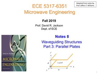
  • 1. Prof. David R. Jackson Dept. of ECE Notes 8 ECE 5317-6351 Microwave Engineering Fall 2019 Waveguiding Structures Part 3: Parallel Plates 1 , ,    x z y d w Adapted from notes by Prof. Jeffery T. Williams
  • 2. 2 2 2 2 z z x c z c z z y c z c z z x z c z z y z c E H j H k k y x E H j H k k x y E H j E k k x y E H j E k k y x                                                       Summary 2 2 c k    2 2 c z k k k   Field Equations (from Notes 6) This table of fields will be useful to us in the present discussion. 2 (kc is always real) (k can be complex) z jk z e 0 1 (1 tan ) (1 tan ) c c c c c c c d r j j j j j j j                                              Assumption:
  • 3. Parallel-Plate Waveguiding Structure  Both plates assumed PEC  w >> d 0 x     The parallel-plate structure is a good approximate model for a wide microstrip line. 3 (neglect edge effects) , w h , ,    c j       , ,    x z y d w PEC
  • 4. 4 TEM Solution Process A) Solve Laplace’s equation subject to appropriate B.C.s.: B) Find the transverse electric field: C) Find the total electric field: D) Find the magnetic field:   2 , 0 x y      1 ˆ ; H z E z      propagation     , , t e x y x y       , , , , z jk z t z E x y z e x y e k k   Note: The only frequency dependence is in the wavenumber kz = k.
  • 5. 2 conductors  1 TEM mode To solve for TEM mode:   2 , 0 x y    Boundary conditions: 0 ( ,0) 0 ; ( , ) x x d V     2 2 2 2 2 0 x y                 TEM Mode z c k j k k jk             k k       5 0 0 x w y d     , ,    x z y d w PEC
  • 6. where ( , ) x y A By    0 ˆ ( , , ) ( , ) jkz jkz t V E x y z e x y e y e d    0 A  2 2 0 y         0 ,0 0 & , x x d V       0 ˆ ˆ , t V e x y y y y d          TEM Mode (cont.) 6 0 V B d  0 ( , ) V x y y d   Hence We then have
  • 7. Recall   0 ˆ , , jkz V H x y z x e d     1 ˆ ( ) H z E     0 ˆ ( , , ) jkz V E x y z y e d   TEM Mode (cont.) 7 c     c j       Fields for +z mode: E H x y 0 V , ,    , ,    x z y d w PEC
  • 8. TEM Mode (cont.) 8 We can view the TEM mode in a parallel-plate waveguiding structure as a rectangular “slice” of a plane wave. The PEC and PMC walls do not disturb the fields of the plane wave. ˆ 0 n E   PEC : ˆ 0 n H   PMC : PEC PEC PMC PMC , ,    x E H y PEC: Perfect Electric Conductor PMC: Perfect Magnetic Conductor
  • 9. Assume a wave propagating the in + z direction henceforth. Time-ave power flow in + z direction:   * 2 0 2 * 2 0 0 2 2 0 2 * 1 ˆ Re ( ) 2 1 ˆ ˆ Re 2 1 1 1 Re 2 s w d k z k z P E H z dS V z z e dydx d V wd e d                                                   2 2 0 * 1 1 Re 2 k z w P V e d                  TEM Mode (cont.) 9   0 0 ˆ ( , , ) ˆ , , jkz jkz V E x y z y e d V H x y z x e d       , ,    x z y d w PEC
  • 10. Transmission line voltage   0 0 ˆ ( ) ( ) d jkz V z E y dy V z V e      Transmission line current   0 top 0 0 0 ( ) , , ( ) w w sz x jk I z I z J dx H x d z dx V I z we d         Characteristic Impedance 0 0 0 jkz jkz V e Z I e    0 d Z w   TEM Mode (cont.) 10 top ˆ ( ) s sz x J n H J H     Note : On PEC on top plate , ,    x z y d w I   V PEC I c     c j      
  • 11. Time-ave power flow in +z direction:   * * 2 0 0 2 2 0 * 1 Re 2 1 Re 2 1 1 Re 2 k z k z P VI V V w e d w P V e d                                        Recall that we found from the fields that: 2 2 0 * 1 1 Re 2 k z w P V e d                  Same TEM Mode (cont.) (calculated using the voltage and current) This is expected, since a TEM mode is a transmission-line type of mode, which is described by voltage and current. 11
  • 12. Recall: where     2 2 2 2 2 , , z c z e x y k e x y x y              ( , , ) ( , ) z jk z z z E x y z e x y e  TMz Modes (Hz = 0) 12     2 2 , , t z c z e x y k e x y    eigenvalue problem 2 2 c z k k k       2 2 2 z c z d e y k e y dy   (Assume no x variation) so Note: Solving the eigenvalue problem (using appropriate boundary conditions) will tell us what the eigenvalue kc is. , ,    x z y d w PEC
  • 13.   sin( ) cos( ) @ 0 0 @ 1,2,... z c c c c e y A k y B k y y B y d k d n n n k d              ApplyB.C.'s : subject to B.C.’s Ez = 0 @ y = 0, d 13     2 2 2 z c z d e y k e y dy   Solving the above equation: TMz Modes (cont.) , ,    x z y d w PEC
  • 14.   sin 1,2,... z n e y A y n d            , sin z jk z z n n E y z A y e d           For a wave propagating in the +z direction: 2 2 2 2 cos cos z z jk z c z c x n c c jk z z z z y n c c j E j n n H A y e k y k d d jk E jk n n E A y e k y k d d                                             1/2 2 1/2 2 2 2 z c n k k k k d                    2 2 c k    TMz Modes (cont.) 14 No x variation TMz mode 0 0 0 x y z E H H   
  • 15. sin z jk z z n n E A y e d          Summary 1/2 2 2 2 2 cos cos 0 ; 1,2,... z z jk z z y n c jk z c x n c x y z c z c jk n E A y e k d j n H A y e k d E H H n k n d n k k d k                                               Each value of n corresponds to a unique TMz field solution or “mode” in the waveguide.  TMn mode Note: 0 0 TM TEM z n k k      15 TMz Modes (cont.) The TEM mode can be thought of as a TM0 mode. , ,    x z y d w PEC
  • 16.   2 1/2 2 2 1/2 2 2 c k z c n k k d k k                        0,1,2,... n  2 2 2 2 2 2 2 2 z z c z c c j z c k z k k k k j k k j e k k k k e                     propagating mode For For Fields decay exponentially  “evanescent” mode Lossless Case c        2 2 k    real 16 TMz Modes (cont.) , ,    x z y d w PEC
  • 17. Cutoff frequency (for lossless case) fc  cutoff frequency @ c f f  c c n k k d       1 2 c cn n f f d    cutoff frequency for TMn mode 17 c      TMz Modes (cont.) Note: For a lossy waveguide, there is no sharp definition of cutoff frequency. This is the frequency that defines the border between evanescence and propagation.
  • 18. Time average power flow in z direction (lossless case):   * 0 0 * 0 0 2 2 2 2 0 1 ˆ Re 2 1 Re 2 Re{ } cos 2 w d TMn w d y x d z z n c P E H z dydx E H dydx n k A w y dy e k d                                2 2 2 Re{ } 2 2 1,2,... z TMn z n c d P k A w e k n            18 c      TMz Modes (cont.) cos cos z z jk z z y n c jk z c x n c jk n E A y e k d j n H A y e k d                     z c z c k k i f f f f   is realfor is maginary for , ,    x z y d w PEC
  • 19. Recall: where     2 2 2 2 2 , , z c z h x y k h x y x y              ( , , ) ( , ) z jk z z z H x y z h x y e  TEz Modes (Ez = 0) 19     2 2 , , t z c z h x y k h x y    eigenvalue problem 2 2 c z k k k       2 2 2 z c z d h y k h y dy   (Assume no x variation) so Note: Solving the eigenvalue problem (using appropriate boundary conditions) will tell us what the eigenvalue kc is. , ,    x z y d w PEC
  • 20. subject to B.C.’s Ex = 0 @ y=0, d 1 y z x c H H E j y z              TEz Modes (cont.) ˆ 0, 0 t H n E    PEC: 20 0 z h y    Solving the above equation:     2 2 2 z c z d h y k h y dy   sin( ) cos( ) cos( ) sin( ) @ 0 0 @ , 1,2,3,... z c c c c c z c c c n h A k y B k y h k A k y k B k y y A n d d k d n k y                 ApplyB.C.'s: , ,    x z y d w PEC
  • 21.   cos 1,2,3,... z n n h y B y n d          2 2 2 2 sin sin z z jk z z x n c c jk z z z z y n c c j H j n n E B y e k y k d d jk H jk n n H B y e k y k d d                                             1/2 2 2 1/2 2 2 z c k k k n k d                    2 2 c k    TEz Modes (cont.) 21   , cos z jk z z n n H y z B y e d          0 0 0 x y z H E E    For a wave propagating in the +z direction: No x variation TEz mode
  • 22. Summary cos z jk z z n n H B y e d          Cutoff frequency 1 2 c cn n f f d          Each value of n corresponds to a unique TEz field solution or “mode.” 1/2 2 2 2 2 sin sin 0 ; 1,2,... z z jk z x n c jk z z y n c x y z c z c j n E B y e k d jk n H B y e k d H E E n k n d n k k d k                                              22 TEz Modes (cont.)  TEn mode Note: There is no TE0 mode (This mode would be a plane wave having Ex and Hy, but would not be supported by this system. This mode would require PMC on top and bottom, and PEC on the sides.) , ,    x z y d w PEC
  • 23.   * 0 0 * 0 0 2 2 2 2 0 1 ˆ Re 2 1 Re 2 Re{ } sin 2 w d TEn w d x y d z z n c P E H z dydx E H dydx n k B w y dy e k d                                    2 2 2 Re 4 z TEn z n c P k B wd e k      Power in TEz Mode Time average power flow in z direction (lossless case): 23 c      sin sin z z jk z x n c jk z z y n c j n E B y e k d jk n H B y e k d                    , ,    x z y d w PEC z c z c k k i f f f f   is realfor is maginary for
  • 24. For all the modes of a parallel-plate waveguiding structure, we have 1 2 cn n f d           The mode with lowest cutoff frequency is called the “dominant” mode of the waveguide. Mode Chart 24 c      Important conclusion: If we want to use the structure as a transmission line, we need to operate in the region f < fc1. TEM TM1 TM2 TM3 Single mode prop. 3 modes prop 5 mode prop. 0 …. TE3 TE2 TE1 f 1 c f 2 c f 3 c f
  • 26. Plane Wave Interpretation 26 sin cos cos z z z jk z z n jk z z y n c jk z c x n c n E A y e d jk n E A y e k d j n H A y e k d                              TMz waveguide mode propagating in +z direction:       sin cos cos z z z jk z z n y jk z z y n y c jk z c x n y c E A k y e jk E A k y e k j H A k y e k         c n k d   Re-label this as ky       1 2 2 2 y y z z y y z z y y z z jk y jk y jk z jk z z n jk y jk y jk z jk z z y n c jk y jk y jk z jk z c x n c E A e e e e j jk E A e e e e k j H A e e e e k                                    1 1 cos sin 2 2 jx jx jx jx x e e x e e j      
  • 27. Plane Wave Interpretation (cont.) 27 The TMz waveguide mode is a sum of two plane waves*:       1 2 2 2 y y z z y y z z y y z z jk y jk y jk z jk z z n jk y jk y jk z jk z z y n c jk y jk y jk z jk z c x n c E A e e e e j jk E A e e e e k j H A e e e e k                            cos z k k     z y   E E H H z TM Side view , ,    x z y d w PEC *We can also think of one a single plane wave bouncing up and down.
  • 28. 28 The TEz waveguide mode is a sum of two plane waves*:           1 2 2 2 y y z z y y z z y y z z jk y jk y jk z jk z z n jk y jk y jk z jk z x n c jk y jk y jk z jk z z y n c H B e e e e j E B e e e e j k jk H B e e e e j k                            Plane Wave Interpretation (cont.)   cos z k k   z y z TE H H E E   Side view , ,    x z y d w PEC *We can also think of one a single plane wave bouncing up and down.
  • 29. Conductor Attenuation on Parallel Plates   * 0 0 0 2 0 2 0 0 2 0 1 ˆ Re 2 1 ˆ ˆ Re 2 1 1 2 w d w d P E H z dydx V z z dydx d w V d                                            0 0 ˆ ˆ jkz jkz V E y e d V H x e d        top 0 ˆ ˆ s jkz J y H V z e d       bot 0 ˆ ˆ jkz s V J y H z e d       On the top plate: On the bottom plate: 29 Assume no dielectric loss for the calculation of conductor attenuation. TEM Mode , Real k   0 (0) 2 l c P P   x z y d w m  c      m 
  • 30. 2 2 top bot 0 0 0 0 (0) 2 w w s l s s z z R P J dx J dx             2 0 0 w s V R dx d    2 0 2 ( ) s V R w d   2 0 2 2 0 0 ( ) (0) 2 1 2 2 s l c w R V d P P w V d                        s c R d    (equal contributions from both plates) The final result is then 30 Conductor Attenuation on Parallel Plates (cont.) We then have: 1 2 2 2 1 1 0 0 1 1 (0) 2 2 l s s s s C C z z P R J d R J d      
  • 31. 31 Let’s try the same calculation using the Wheeler incremental inductance rule. cond 0 0 2 s c R Z Z            0 d Z w         From previous calculations: top bot c c c      0 0 Z dZ d     ( d   for eitherplate) since Conductor Attenuation on Parallel Plates (cont.) ,   , Real k   w d In this formula, (for a given conductor) is the distance by which the conducting boundary is receded away from the field region. We apply the formula for each conductor and then add the results:
  • 32. s c R d    32 cond 0 0 2 s c R Z Z            0 d Z w         0 0 Z dZ d     top 0 0 2 2 2 2 s s s s c R R R R d d Z d w wZ d w w                              bot 0 0 2 2 2 2 s s s s c R R R R d d Z d w wZ d w w                              Hence, we have: Conductor Attenuation on Parallel Plates (cont.) ,   , Real k   w d
  • 33. 33 Surface Roughness Conductor attenuation will increase due to surface roughness effects. ① ② ③ ④ 200 m Surfaces 3 and 4 are rough. Stripline
  • 34. 34 Surface Roughness (cont.) We can use an effective conductivity to account for surface roughness.   7 3.0 10 S/m    Pure copper   7 5.8 10 S/m    Practical copper Example:
  • 35. 35 Surface Roughness (cont.) https://www.microwaves101.com/encyclopedias/surface-roughness 2 1 rough 2 1 tan 1.4 a R K                    Hammerstad and Jensen formula E. Hammerstad and O. Jensen, “Accurate models for microstrip computer-aided design,” in Microwave Symp. Digest, IEEE MTT-S International, 1980, vol. 1, no. 12, pp. 407–409. Attenuation factor Krough vs. surface roughness Attenuation factor Ratio of roughness Ra to skin depth  This is a factor that gives the increase in the attenuation constant . Ra = height of surface roughness
  • 36. 36 Surface Roughness (cont.) r r Ar rbase … … Ar: Hemispheroid height rbase: Hemispheroid radius r: Period X. Guo, D. R. Jackson, M. Y. Koledintseva, S. Hinaga, J. L. Drewniak, and J. Chen, “An Analysis of Conductor Surface Roughness Effects on Signal Propagation for Stripline Interconnects,” IEEE Trans. Electromagnetic Compatibility, Vol. 56, No. 3, pp. 707–714, June 2014. base / 1/ 3 r r  
  • 37. Results for TM/TE Modes (above cutoff): (derivation omitted) TMn modes of PPW: TM 2 , 0 s cn kR n d     TEn modes of PPW: 2 TE 2 , 0 c s cn k R n k d     37 Note: Below cutoff, we usually do not worry about conductor loss. Conductor Attenuation on Parallel Plates (cont.) Waveguide Modes x z y d w m  c      m 