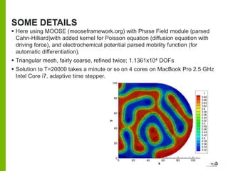
BENCHMARK 6 UPDATE
drhgfdjhngngfmhgmghmghjmghfmf
OLLE HEINONEN, ANDREA JOKISAARI, JIM WARREN, JON GUYERS, PETER VOORHEES
Sept. 25, 2018
Center for Hierarchical Materials Design http://chimad.northwestern.edu/about/index.html
BACKGROUND
 Benchmark 6 is a simple model of flow of a charged concentration field.
 Technically, it is a coupled Cahn-Hilliard-Poisson problem: the concentration field
flows under forcing of an electrochemical potential which contains contributions from
the electrostatic field generated by the charge distribution.
 Previous formulation was unsatisfactory:
– One one type of charge so the system was not charge-neutral.
– Original model was technically identical to a block co-polymer problem –
desirable to make it a little different
 The boundary conditions (zero flow of concentration field across boundaries,
Dirichlet BC for the electrostatic field) where not quite physical: the particle flow and
charge flow are linked (Einstein relation) so a particle flow across boundary has to
have a concomitant charge flow across boundary.
 It is desirable (but not absolutely necessary) to have the total energy of the system
be monotonically non-increasing. This is generally not the case if there is flow
across the the boundaries (external field does work on the system).
2
New formulation
 Same geometries: (i) square 100 x 100 units, and square+halfmoon (rectangle
50 x 100 units and half-circle radius 50 nm attached)
 Concentration-dependent mobility 𝑀 𝑐 =
𝑀0
1+𝑐2 to make it a little bit more
interesting (also rather physical for ionic flow).
 Neutralizing uniform background charge density 𝑐0 with total magnitude of
charge same as initial total charge of concentration field 𝑐
 Applied external field Φ 𝑒𝑥𝑡 such that ∇2
Φ 𝑒𝑥𝑡=0.
 Zero particle and charge flow across boundaries.
 Pseudo-random initial concentration field with average concentration close to 0.5
3
FREE ENERGY
 Free energy contains contributions from bulk chemical energy, gradient in the
concentration field (standard spinodal decomposition), and electrostatic free
energy:
𝑓𝑒𝑙𝑒𝑐=
1
2
𝜌Φ𝑖𝑛𝑡 + 𝜌 Φ 𝑒𝑥𝑡
where Φ 𝑡𝑜𝑡= Φ𝑖𝑛𝑡 + Φ 𝑒𝑥𝑡 is the total electrostatic potential, and 𝜌 = 𝑘 𝑐 − 𝑐0 with k
a constant
4
EQUATIONS
The equations to be solved are then
where Φ = Φ 𝑡𝑜𝑡=Φ𝑖𝑛𝑡+ Φ 𝑒𝑥𝑡 because it was easy to copy latex images and I hate
writing equations using ppt.
Boundary conditions:
 No particle current across boundaries ∇𝜇 ∙ 𝑛=0
 No charge current across boundary:
 External potential Φ 𝑒𝑥𝑡 = 𝐴𝑥𝑦 + 𝐵𝑥 + 𝐶𝑦
5
SOME DETAILS
 Here using MOOSE (mooseframework.org) with Phase Field module (parsed
Cahn-Hilliard)with added kernel for Poisson equation (diffusion equation with
driving force), and electrochemical potential parsed mobility function (for
automatic differentiation).
 Triangular mesh, fairly coarse, refined twice; 1.1361x10⁴ DOFs
 Solution to T=20000 takes a minute or so on 4 cores on MacBook Pro 2.5 GHz
Intel Core i7, adaptive time stepper.
6
SOME SANITY CHECKS (MOOSE)
 First set Dirichlet BC on total
potential, Φ 𝑡𝑜𝑡 = 0 on
boundaries, Φ 𝑒𝑥𝑡=0
7
Then use Neumann conditions on
electrostatic potential, Φ 𝑒𝑥𝑡=0
Note that Neumann BC are integrated
in MOOSE: the BC is not satisfied at all
points, but only the integral over each
boundary.
MORE SANITY CHECKS
8
Tune the relative strength of electrostatic to chemical forces with
the dielectric constant 𝜀. For 𝜀 = 1 electrostatic energy large so
system should go to uniform density for minimal electrostatic
energy
Already at timestep T=20 the concentration field is uniform
…and more
 For 𝜀 = 100 the electrostatic energy is insignificant compared to chemical
energy. System should do spinodal decomposition.
9
Increase mobility by factor of 2, extend
time to T=20000
With external potential
10
Here at T=1500
Concentration field (Total) Electrostatic potential
Laplacian of potential −𝑘(𝑐 − 𝑐0)/𝜀
Tuning dielectric constant (T=1500)
11
𝜀 = 10
𝜀 = 5
𝜀 = 2
 Re-formulated coupled Cahn-Hilliard-Poisson problem to make it a little bit more
physical
 A few simple tests to see if solution makes sense
 Note: Solutions I use pass smell-test but not sure about calculation of total
energy (which is why I did not show any total energy plots). For that matter, there
could be other bugs, too…..
 Runs very fast with
12
Summary
OUTLINE
13
www.anl.gov

Benchmark 6 Update

  • 1.
    BENCHMARK 6 UPDATE drhgfdjhngngfmhgmghmghjmghfmf OLLEHEINONEN, ANDREA JOKISAARI, JIM WARREN, JON GUYERS, PETER VOORHEES Sept. 25, 2018 Center for Hierarchical Materials Design http://chimad.northwestern.edu/about/index.html
  • 2.
    BACKGROUND  Benchmark 6is a simple model of flow of a charged concentration field.  Technically, it is a coupled Cahn-Hilliard-Poisson problem: the concentration field flows under forcing of an electrochemical potential which contains contributions from the electrostatic field generated by the charge distribution.  Previous formulation was unsatisfactory: – One one type of charge so the system was not charge-neutral. – Original model was technically identical to a block co-polymer problem – desirable to make it a little different  The boundary conditions (zero flow of concentration field across boundaries, Dirichlet BC for the electrostatic field) where not quite physical: the particle flow and charge flow are linked (Einstein relation) so a particle flow across boundary has to have a concomitant charge flow across boundary.  It is desirable (but not absolutely necessary) to have the total energy of the system be monotonically non-increasing. This is generally not the case if there is flow across the the boundaries (external field does work on the system). 2
  • 3.
    New formulation  Samegeometries: (i) square 100 x 100 units, and square+halfmoon (rectangle 50 x 100 units and half-circle radius 50 nm attached)  Concentration-dependent mobility 𝑀 𝑐 = 𝑀0 1+𝑐2 to make it a little bit more interesting (also rather physical for ionic flow).  Neutralizing uniform background charge density 𝑐0 with total magnitude of charge same as initial total charge of concentration field 𝑐  Applied external field Φ 𝑒𝑥𝑡 such that ∇2 Φ 𝑒𝑥𝑡=0.  Zero particle and charge flow across boundaries.  Pseudo-random initial concentration field with average concentration close to 0.5 3
  • 4.
    FREE ENERGY  Freeenergy contains contributions from bulk chemical energy, gradient in the concentration field (standard spinodal decomposition), and electrostatic free energy: 𝑓𝑒𝑙𝑒𝑐= 1 2 𝜌Φ𝑖𝑛𝑡 + 𝜌 Φ 𝑒𝑥𝑡 where Φ 𝑡𝑜𝑡= Φ𝑖𝑛𝑡 + Φ 𝑒𝑥𝑡 is the total electrostatic potential, and 𝜌 = 𝑘 𝑐 − 𝑐0 with k a constant 4
  • 5.
    EQUATIONS The equations tobe solved are then where Φ = Φ 𝑡𝑜𝑡=Φ𝑖𝑛𝑡+ Φ 𝑒𝑥𝑡 because it was easy to copy latex images and I hate writing equations using ppt. Boundary conditions:  No particle current across boundaries ∇𝜇 ∙ 𝑛=0  No charge current across boundary:  External potential Φ 𝑒𝑥𝑡 = 𝐴𝑥𝑦 + 𝐵𝑥 + 𝐶𝑦 5
  • 6.
    SOME DETAILS  Hereusing MOOSE (mooseframework.org) with Phase Field module (parsed Cahn-Hilliard)with added kernel for Poisson equation (diffusion equation with driving force), and electrochemical potential parsed mobility function (for automatic differentiation).  Triangular mesh, fairly coarse, refined twice; 1.1361x10⁴ DOFs  Solution to T=20000 takes a minute or so on 4 cores on MacBook Pro 2.5 GHz Intel Core i7, adaptive time stepper. 6
  • 7.
    SOME SANITY CHECKS(MOOSE)  First set Dirichlet BC on total potential, Φ 𝑡𝑜𝑡 = 0 on boundaries, Φ 𝑒𝑥𝑡=0 7 Then use Neumann conditions on electrostatic potential, Φ 𝑒𝑥𝑡=0 Note that Neumann BC are integrated in MOOSE: the BC is not satisfied at all points, but only the integral over each boundary.
  • 8.
    MORE SANITY CHECKS 8 Tunethe relative strength of electrostatic to chemical forces with the dielectric constant 𝜀. For 𝜀 = 1 electrostatic energy large so system should go to uniform density for minimal electrostatic energy Already at timestep T=20 the concentration field is uniform
  • 9.
    …and more  For𝜀 = 100 the electrostatic energy is insignificant compared to chemical energy. System should do spinodal decomposition. 9 Increase mobility by factor of 2, extend time to T=20000
  • 10.
    With external potential 10 Hereat T=1500 Concentration field (Total) Electrostatic potential Laplacian of potential −𝑘(𝑐 − 𝑐0)/𝜀
  • 11.
    Tuning dielectric constant(T=1500) 11 𝜀 = 10 𝜀 = 5 𝜀 = 2
  • 12.
     Re-formulated coupledCahn-Hilliard-Poisson problem to make it a little bit more physical  A few simple tests to see if solution makes sense  Note: Solutions I use pass smell-test but not sure about calculation of total energy (which is why I did not show any total energy plots). For that matter, there could be other bugs, too…..  Runs very fast with 12 Summary
  • 13.
  • 15.