Demystifying LTE Performance Management and Optimization

Demystifying LTE
Management
Opeyemi Praise, Senior LTE RF
Limited, Victoria Island, Lagos, Nigeria.
Demystifying LTE Performance
Management and Optimization
White Paper
, Senior LTE RF/RAN Engineer, Cyberspace Network
Limited, Victoria Island, Lagos, Nigeria.
April 2015
Performance
and Optimization
Engineer, Cyberspace Network

ABSTRACT
This report captures the procedures, processes, thought and skills required
in the KPI (Key Performance Indices) analysis of industry fastest data
network, the LTE network. It is aimed at showcasing professional
experience acquired over the years in the field of Access Network
Planning and Optimization, which is a specialization within the
Telecommunication field.
The report explains, to the finest details, processes and work flow for
monitoring and analysis of KPI’s in the LTE network. It takes you through the
different KPI’s of the LTE network, how they are measured, how they are
monitored, their threshold, their meaning and implications at different
levels and how they can be optimized, amongst other things.
It promises to give readers both basic and in-depth understanding of KPI
analysis of telecommunication access network; the knowledge can be
extrapolated to other access technologies.
It should be noted that Huawei Technologies performance management
tool was used in this report.

ACKNOWLEDGEMENT
My profound gratitude goes to my heavenly Father. He alone has been
the source of my strength and wisdom.
I appreciate my wife, the one who is always there when challenges
come. She is always there to encourage and provide needed support
that no one can.
I must appreciate the fatherly counsel of my mentor, Engr. Nwalune
Augstine, Director of Spectrum Administration, Nigeria Communications
Commission (NCC). I have been privileged to work with some of the best
bosses one can pray for; their contribution has helped my career a great
deal – Engr. Azikiwe Chukwunedum, Engr. Fred Young, Engr. Azubike
Osunwa, Engr. Joe Onwubuya and Mr. Ye Guohong
My profound gratitude goes to my parents for the sacrifices paid to have
me educated. I also appreciate the moral and emotional support given
by my wife since we have met. My appreciation also goes to highly
respected senior colleagues in the field; Engr. Nathan Ndifreke, Engr.
Olayinka Bolade and Engr. Babatunde Duntoye who painstakingly guided
the preparation of this report. The correction and suggestions from various
reviews has produced this report.

I must acknowledge my supervisors, managers, mentors and colleagues
who gave me the opportunity to learn, trained me and assigned tasks
that matured me to this level. I also appreciate my subordinates who
have been instrumental to the success of my career, especially in project
delivery and managed service.
Big appreciation to Huawei Technologies for pioneering leadership in the
telecom equipment vendor industry. Huawei has indeed made great
innovations in the industry.

Chapter 1
INTRODUCTION
1.1 Background
LTE (Long-Term Evolution, commonly marketed as 4G LTE) is a standard
for wireless communication of high-speed data for mobile phones and
data terminals. It is based on the GSM/EDGE and UMTS/HSPA network
technologies, increasing the capacity and speed using a different radio
interface together with core network improvements. The standard is
developed by the 3GPP (3rd Generation Partnership Project).
Technologies (2G and 3G) before now are limited in speed, latency and
simplicity of architecture. LTE comes with the following benefits;
1. Cost Reduction – more value for investment on infrastructure since
LTE has higher spectrum efficiency hence lower operations cost per
bit. More bits are transmitted and received at a lower cost.
2. Next Generation Applications – because LTE offers high speed and
low latency, it can be used to power next generation applications
such as Mobile-TV, Online gaming, VoIP, Video-on-demand etc.
These applications are data hungry.

3. Simplified Network Architecture – LTE has fewer network elements
and migrations path, hence it is easy to deploy and cheaper than
the legacy technologies.
4. Scalable Bandwidth - LTE can run on wide range of bandwidth
depending on the one that fits the operator technological and
business model. The following bandwidth can run on LTE: 1.25MHz,
3MHz, 5MHz, 10MHz, 15MHz and 20MHz.
5. Mobility at High Speed - With LTE, you can have uninterrupted
connection moving at high speed of about 350Km/h, this is not
possible with other technology.
1.2 Project Description
This report is aimed at demystifying the LTE technology and narrowed
down to performance management of the modern telecommunication
infrastructure. The performance management of the LTE network involves
KPI monitoring and analysis, and then optimization, if KPIs are outside the
expected acceptable thresholds.
1.3 Scope of Work
For volume and simplicity reasons, this report captures the basic
understanding of the LTE architecture and details on KPI analysis of the
network (performance management).

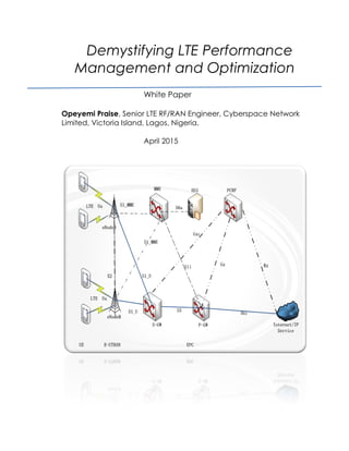
Chapter 2
LTE ARCHITECTURE
The LTE network has interconnectivity of different network elements each
of which has its own function. This chapter captures each of the network
elements, their functions and the interconnecting interfaces.
Figure 2.1: LTE Network Architecture Diagram

2.1 Functions of LTE Network Elements
Figure 2.1 above shows the LTE Network Architecture. The network is
basically in two parts. The E-UTRAN and the EPC. The E-UTRAN (Evolved
Universal Terrestrial Radio Access Network) is the access part of the
network and consist of eNodeB’s. UE (User Equipment) accesses the
network by searching and demodulating signals from the closest eNodeB
with the best signal strength.
The other part of the network, EPC (Evolved Packet Core) is made up of
the core network equipment such as;
1. MME – Mobility Management Entity. MME is the key control node for
LTE access network. It is responsible for tracking and paging
procedure including retransmissions, and also for idle mode of User
Equipment (UE). MME is also involved in bearer activation and its
deactivation procedures, its task also belongs to choosing the SGW
for a UE in process of initial attach and when the intra-handover
take place which involves Core Network (CN) node relocation.
2. HSS – Home Subscriber Server. The HSS is the concatenation of the
HLR (Home Location Register) and the AuC (Authentication Center)
– two functions being already present in pre-IMS 2G/GSM and
3G/UMTS networks. The HLR part of the HSS is in charge of storing

and updating when necessary the database containing all the user
subscription information, such as IMSI (International Mobile
Subscriber Identity), MSISDN (Mobile Subscriber ISDN Number) or
mobile telephone number, user profile etc.
3. PCRF – Policy and Charging Rule Function. PCRF is the node
designated in real-time to determine policy rules in the network. As
a policy tool, the PCRF plays a central role in next-generation
networks. Unlike earlier policy engines that were added onto an
existing network to enforce policy, the PCRF is the component that
operates at the network core and accesses subscriber databases
and other specialized functions, such as a charging system, in a
centralized manner. Because it operates in real time, the PCRF has
an increased strategic significance and broader potential role than
traditional policy engines.
4. S-GW – Serving Gateway. Serving GW is the gateway which
terminates the interface towards E-UTRAN. For each UE associated
with the EPS, at given point of time, there is a single Serving GW.
SGW is responsible for handovers with neighbouring eNodeB's, also
for data transfer in terms of all packets across user plane. Its duties
belong to taking care of mobility interface to other networks such
as 2G/3G.

5. P-GW – Packet Data Network Gateway. The PGW is the gateway
which terminates the SGi interface towards PDN. If UE is accessing
multiple PDNs, there may be more than one PGW for that UE,
however a mix of S5/S8 connectivity and Gn/Gp connectivity is not
supported for that UE simultaneously. PGW is responsible to act as
an "anchor" of mobility between 3GPP and non-3GPP technologies.
PGW provides connectivity from the UE to external PDN by being
the point of entry or exit of traffic for the UE. The PGW manages
policy enforcement, packet filtration for users, charging support
and LI (Legal Interception).

Chapter 3
LTE ACCESS NETWORK KPI
This chapter specifies a set of evolved Radio Access Network (eRAN) KPIs
to evaluate the performance of the LTE system; ‘evolved’ means an
advancement from the legacy networks (UMTS, GSM, CDMA, ie 2G, 3G
ect). This chapter reveals the different KPIs that can be used to measure
the performance of the LTE network, how they are calculated and their
significance. Some counters necessary for the KPI calculation are also
described in details.
3. 1 The LTE Access Network
The access network is a network of base station radios (arranged to cover
a specific geographical area) in connection together (by most cost
effective transport media) to the core. The access network is that part of
the telecoms network that provide coverage signal to subscribers so they
can connect to telecoms services.
The access network KPIs are classified into categories based on the
measurement targets: accessibility, retainability, mobility, service integrity,
utilization, availability, and traffic KPIs.

3.1.1Access Network Accessibility
Accessibility KPIs are used to measure the probability whether services
requested by a user can be accessed within specified tolerances in the
given operating conditions. The service provided by the E-UTRAN is
defined as EPS/ERABs. Radio Resource Control (RRC) connection and
System Architecture Evolution (ERAB) setup are the main procedures for
accessibility KPIs. The accessibility KPIs can be calculated per cell or
cluster. The KPIs at the cluster level are calculated by aggregating all cell
counters of the same cluster.
3.1.1.1 RRC Setup Success Rate
The KPI is calculated based on the counters measured at eNodeB when
the eNodeB receives an RRC Connection Request from the UE, as shown
in Figure 3.1. To illustrate the KPI calculation procedures, we briefly discuss
how the related counters (number of RRC Connection setup attempts
(service) and number of successful RRC setup (service)) are collected. The
number of RRC Connection attempts is collected by the eNodeB at
measurement point A and the number of successful RRC connection is
counted at measurement point C. The higher the RRC Setup Success
Ratio the healthier the network. Low values indicate that there is an issue
with the network.

Figure 3.1: Signal Flow for Measurement of RRC Setup Success Ratio
Mathematically, RRC Setup Success Ratiois defined in the table below.
Table 3.1; Mathematical Definition of RRC Setup Success Ratio
3.1.1.2 ERAB Setup Success Rate (VoIP)
E-UTRAN Radio Access Bearer (ERAB) is the signaling path for data traffic
coming from the RAN. ERAB carries the data traffic from the RAN and

delivers it to the Evolved Packet Core (EPC); the EPC is also called Evolved
Packet System (EPS). The EPC is that part of the network where User
Equipment (UE) from the RAN is controlled and enabled to access services
hosted at the EPC. Figure 3.2 shows the signal flow of ERAB Setup Success
Rate.
ERAB Setup Success Rate measures the fact that the UE can now connect
to EPC. The higher the rate the healthier the network. Poor values of ERAB
Setup Success Rate means UE’s are having issues connecting to the EPC;
please bear in mind that the EPC contains the MME, UGW, P-GW, PCRF
etc.
Figure 3.2; Signal Flow for Measurement of ERAB Setup Success Rate
Mathematically, ERAB Setup Success Rate is defined in the Table 3.2
below.

Table 3.2; Mathematical Definition of ERAB Setup Success Ratio
3.1.1.3 Call Setup Success Rate (CSSR)
The Call Setup Success Rate (CSSR) is the KPI that measure the combined
accessibility experience of users. It merges the impact of RRC Setup
Success Ratio with ERAB Setup Success Rate. Table 3.2 below shows the
mathematical representation of CSSR.
Table 3.2; Mathematical Definition of Call Setup Success Ratio
3.1.2 Access Network Retainability
Retainability KPIs are used to evaluate the network capability to retain
services requested by a user for a desired duration once the user is
connected to the services. These counters can be calculated per cell or
per cluster. The KPIs at the cluster level can be calculated by aggregating

all the cell counters. Retainability KPIs are important in evaluating whether
the system can maintain the service quality at certain level
3.1.2.1 Call Drop Rate (VoIP)
This KPI can be used to evaluate the call drop rate of the VoIP service in a
cell or a cluster. The call drop rate is calculated by monitoring the VoIP
ERAB abnormal release rate. ERAB includes both the ERAB radio bearer
and corresponding S1 bearer. Any abnormal release on either bearer
causes call drop and therefore is counted into the call drop rate. The Call
Drop Rate (CDR) is defined as Abnormal ERAB release / All released ERAB.
It should be noted that the lower the CDR, the healthier the network. High
CDR means, many subscribers have been abnormally dropped within the
hour(s) of monitoring.
Figure 3.3; Signal Flow for Measurement of Call Drop Rate (VoIP)
Mathematically, CDR_VoIP is defined as in Table 3.3 below.

Table 3.3; Mathematical Calculations of Call Drop Rate.
3.1.3 Access Network Mobility
Mobility KPIs are used to evaluate the performance of E-UTRAN mobility,
which is critical to the customer experience. Several categories of mobility
KPIs are defined based on the following handover types: intra-frequency,
inter-frequency, and inter-Radio Access Technology (RAT).
3.1.3.1 Intra-frequency Handover Out Success Rate
This KPI can be used to evaluate the intra-frequency Handover out
success rate in a cell or a cluster. The intra-frequency handover (HO)
includes both inter-eNodeB and intra-eNodeB scenarios. To illustrate the
KPI calculation, we briefly discuss how the related counters (number of
intra-frequency HO attempts and number of successful intra-frequency
HO attempts) are collected. Table 3.4 show the signal flow for Intra-
Freqeucncy Handover-Out Success Rate.

Figure 3.4; Signal Flow for the Meaurement of Intra-Frequency Handover-
Out Success Rate
Mathematically, Intra-frequency Handover Out Success Rate is defined in
Table 3.4 below.
Table 3.4; Mathematical Calculation for the Meaurement of Intra-
Frequency Handover-Out Success Rate
3.1.3.2 Inter-frequency Handover Out Success Rate

Similar to Intra-frequency Handover Out Success Rate, the target eNodeB
and source eNodeB are at different frequencies. This KPI can be used to
evaluate the inter-frequency handover out success rate in a cell or a
cluster. Note that the measurement points for the associated counters are
the same as those for the intra-frequency HO scenario.
Mathematical representation for Inter-Frequency Handover Out is as
below in Table 3.5.
Table 3.5; Mathematical Calculation for the Meaurement of Inter-
Frequency Handover-Out Success Rate
3.1.3.3 Handover In Success Rate
This KPI can be used to evaluate the handover in success rate in a cell or
a cluster. The HO includes both inter-eNodeB and intra-eNodeB scenarios.

To illustrate the KPI calculation, we briefly discuss how related counters
(number of HO attempts and number of successful HOs) are collected.
The eNodeB counts the number of successful intra-eNodeB HOs in the
target cell when the eNodeB receives an
RRCConnectionReconfigurationComplete message from the UE. Figure
3.5 shows the signal flow for Handover in Success Rate.
Figure 3.5; Handover In Success Rate
Mathematically, Handover In Success Rate is as below.
Table 3.6; Mathematical Calculation for Handover-In Success Rate

3.1.4 Access Network Utilization
Utilization KPIs are used to evaluate the capability to meet the traffic
demand and other characteristics in specific internal conditions.
3.1.4.1 Resource Block Utilizing Rate
Resource Block is a network resource assigned to users by scheduler
based on demand for speed and network resource. This KPI consists of
two sub-KPIs: uplink resource block (RB) utilizing rate and downlink RB
utilizing rate. These two sub-KPIs can be used to evaluate the busy-hour DL
and UL RB utilizing rate in each cell or cluster. Table 3.7 below shows the
mathematical representation of RB Utilization Rate.
Table 3.7; Mathematical Calculation for Resource Block Utilizing Rate

3.1.4.2 Average CPU Load
The CPUs of each of the network elements are a resource to be
monitored and optimized when they have reached certain threshold. If
the CPU was allowed to exceed capacity, the Network Element (NE) will
not be able to process subsequent data and subscriber experience will
degrade. Table 3.8 shows Average CPU Load mathematical
representation.
Table 3. 8; Mathematical Calculation for Average CPU Load
3.1.5 Access Network Availability
Availability is the percentage of time that a cell is available. A cell is
available when the eNodeB can provide EPS bearer services. Availability

can be measured at the cell level for a variety of hardware/software
faults.
3.1.5.1 Radio Network Unavailability Rate
The radio network unavailability rate is defined in Table 8-1. This KPI is
calculated based on the time of all cell service unavailability on the radio
network (cluster).
Table 3. 9; Mathematical Calculation for Radio Network Unavailabilty Rate
3.1.6 Access Network Traffic KPI
Traffic KPIs are used to measure the traffic volume on the LTE Radio
Access Network (RAN). Based on traffic types, the traffic KPIs are classified
into the following categories: radio bearers, downlink traffic volume, and
uplink traffic volume.

3.1.6.1 Average User Number
This KPI evaluate the average number of users which has the RRC
connection in the cell. This value is calculated based on samples, eNodeB
will record the user number in the cell to be a sample every second, and
then calculate the average value of these samples in the measurement
period. Table 3.10 shows mathematical representation for Average User
Number.
Table 3. 10; Mathematical Calculation for Average User Number
3.1.6.2 Maximum User Number
This KPI evaluates the maximum number of users which has the RRC
connection in the cell in a period. This value is calculated based on
samples, eNodeB will record the user number in the cell to be a sample
every second, and then get the maximum value of these samples in the
measurement period.

Table 3. 11; Mathematical Calculation for Maximum User Number

Chapter 4
LTE NETWORK PERFOMANCE MONITORING AND ANALYSIS
The network Key Performance Indicators are routinely checked against
threshold. Degradation is when the KPI is lower than threshold in the case
of CSSR, or higher than threshold in the case of CDR. Degradation in KPI
(of a particular NE or Network Segment) shows there is an issue to attend
to. Further analysis reveal what the issue is and rectification or optimization
is done. Table 4.1 below shows the classifications of LTE Network KPI
degradation monitoring.
Table 4.1; Classification of LTE Network KPI Based on Degradation
Monitoring.
*High Value of KPI means Network is fine
*Low Value of KPI means there is an issue
*Low Value of KPI means Network is fine
*High Value of KPI means there is an issue
RRC Setup Success Rate (%) Call Drop Ratio (%)
ERAB Setup Success Rate (%) Resource Block Utilization (%)
Call Setup Success Rate (%) Average CPU Load (%)
Intra-Frequency Handover-Out Success Rate (%)
Inter-Frequency Handover-Out Success Rate (%)
Handover-In Success Rate (%)
Network Availability (%)
Degradation Monitoring

Table 4.2; the table below shows KPI and their threshold.
Network monitoring reveals the area of the network that has issues by
indicating degraded KPI. From the degraded KPI, the root cause analysis
is done. This analysis tells the many things that might be responsible for the
issue and narrows it down to a specific cause(s). This could either be a
hardware that needs upgrade (over utilized), malfunctioning hardware or
a network parameter that needs to be optimized.
4.1 Monitoring LTE Network KPI with M2000
KPI monitoring is very essential in Network Operations. If KPI’s are not
monitored, one cannot ascertain the state of the network, hence quality
of experience of valued subscribers will suffer. For Huawei-built network,
M2000 is a Network Management Tool. This part of the report deals with
how to use M2000.
S/N KPI Threshold (%)
1 RRC Setup Success Ratio (%) 98
2 ERAB Setup Success Ratio (%) 98
3 Call Setup Success Ratio (%) 98
4 Intra-Frequency Handover-Out Success Rate (%) 95
5 Inter-Frequency Handover-Out Success Rate (%) 95
6 Handover-In Success Rate (%) 95
7 Network Availability (%) 99
8 Call Drop Ratio (%) 1.5
9 Resource Block Utilization (%) 70
10 Average CPU Load (%) 70

4.1.1 Logging into M2000
After an account has been created on M2000, log in to M2000 with your
log in credentials.
You should be on the same network segment. The Log in interface for
M2000 is as below in Figure 4.2.
Figure 4.2; Log-in Interface of Huawei M2000
4.1.2 Application Centre
After a successful log in, you are in Application Centre. The Application
Centre (shown in Figure 4.3) display groups of high-level functions in tiles.
From the array of tiles, you choose the function group that applies to the
task you are about to perform.

There are a number task that is directly relevant to KPI Monitoring and
Analysis and they are;
a. Fault Management
b. Trace and Maintenance
c. Wireless and CN Performance
Figure 4.3; showing Application Centre after Log-in to M2000.
4.1.2.1 Fault Management
The fault management gives you the information about alarms on the
network, occurrence time, occurrence duration, frequency of occurrence
and the likes. It the interface for Alarm Management and Analysis.

From Application Center, simply select Fault Management. The Fault
Management (shown in Figure 4.4) shows you all the alarms on the
network in real time, their sources, frequency of occurrence time,
clearance time, Severity and all related information on each alarm. The
fault management also shows history alarms. All alarms are logged in
archive and can be retrieved for analysis.
Figure 4.4; showing Alarms Management Interface of Fault Management
4.1.2.2 Trace and Maintenance
The Trace and Maintenance function gives the access to each RAN
device one-on-one. One can observe the device in real time with the
graphical interface. The Trace and Maintenance (shown in Figure 4.5)
gives access to functions such as Device Panel, Signaling Tracing and
Maintenance.

Figure 4.5; showing Trace and Maintenance Interface
4.1.2.3 Device Panel
It gives you maintenance and monitoring access to each unit network
element in the RAN (each eNodeB, their boards and all). Boards on the
eNodeB can be observed and troubleshooted from the Device Panel
interface (shown in Figure 4.6)
Figure 4.6; showing Device Plane Interface of Trace and Maintenance

4.1.2.4 Signaling Tracing
This interface (as shown in Figure 4.7) provides you access to trace
subscriber signaling information such as Channel Quality, DL RSRP,
Through-put etc.
Figure 4.7; showing the Interface for Signaling Tracing
4.1.2.5Maintenance
This interface (shown in Figure 4.8) provides access to command line
interface of the M2000. With the CLI, you can configure/modify network
parameters of each element on the network.

Figure 4.8; showing the Command Line Interface
4.1.2.6 Wireless and CN Performance
This is the interface (Figure 4.9) that one can generate network KPI’s (that
was dealt with in chapter 3). On M2000, KPI’s are presented as counters or
as a ready (complete data). For KPI’s presented as data counter, the
resultant KPI is calculated using the formula (as stated in chapter 3) on the
constituent counters.
Take for instance to find CDR (Call Drop Rate) for all the cells on the
network, select the CDR template that contains the required counters for
the calculation of CDR as shown below;

Figure 4.9; showing KPI Query
From the CDR templates, two templates are required to get CDR, that is,
ERAB Normal Release and ERAB Abnormal Release. The template allows
to select the time window one is interested in, (like start time 11/01/2016
13:00 to end time 12/01/2016 14:00). The output of the query is as below in
Figure 4.10 below.
The output can be save (in excel format) and a column can be opened
for CDR. The CDR formula is used in the column as in Figure 4.11.

Figure 4.10; showing output of KPI Query
The CDR for each of the Cells at the specific period is shown in the CDR
column. The figure below shows details;
Figure 4.11; showing the processed Query Output for CDR

To find the CDR for the whole cells (in a cluster or in the network), the
cumulative Abnormal Releases and Normal Releases are calculated; this
is then used to find the CDR (for the cluster or the whole network). The use
of Pivot table in excel will found handy in this analysis.
4.2 LTE KPI Analysis
The essence of KPI monitoring is to gather information as per the health
and performance of the network. When KPI exceed the threshold, it might
be an indication of a network issue. Some of the issues might be faulty
network elements, congestion at some network nodes, poor coverage
etc. a detailed analysis gives good information as per the network
performance and hence appropriate solution is found to the issues.
4.2.1 LTE KPI Thresholds
It is important to know what the thresholds are and how to interpret them.
When KPI’s exceed their targets, this is indicative there is an issue. Table 4.3
below shows the LTE KPI’s and their corresponding thresholds.

Table 4.3; showing KPI’s, their thresholds and observations
4.2.2 Root Cause Analysis
Poor KPI is an indication that there are issue on the network which is
usually service impacting. Subscribers experience service degradation
when service impacting issues are on the network, hence, poor Quality of
Experience. To forestall this, KPI’s are monitored and analyzed to find the
root cause. The root cause is then addressed to restore the customer
Quality of Experience.
To carry out root cause analysis, the following should be done;
1. KPI Monitoring
2. Cause Analysis
3. Solution Proposal
4. Post Resolution Monitoring
KPI Threshold Observation
RRC Setup Success Rate (%) 95%
Values higher than 95% are perfect. Values lower than
95% is indicative of network issues.
ERAB Setup Success Rate (%) 95%
Call Setup Success Rate (%) 95%
Intra-Frequency Handover-Out Success Rate (%) 90%
Inter-Frequency Handover-Out Success Rate (%) 90%
Handover-In Success Rate (%) 90%
Network Availabilty (%) 98%
Call Drop Ratio (%) 1.50%
Values lower than 1.5% are perfect. Values higher than
1.5% are indicative of network issues.
Resource Block Utilization (%) 70%
Values lower than 70% are perfect. Values higher than
70% are indicatve of high load on the network.
Network congestion solutions should be explored.
Average CPU Load (%) 70%
Values lower than 70% are perfect. Values higher than
70% are indicatve of high load on the network.
Network congestion solutions should be explored.

4.2.1.1 KPI Monitoring
The LTE Network KPIs are monitored against the threshold as often as daily
or weekly (basically routine network monitoring is done base on company
network policy). When KPI exceed set thresholds, then a cause analysis is
done.
Take for instance, the CDR table above, all the cell have KPI’s within the
acceptable range (not exceeding the threshold), hence, there is no need
to do a Cause Analysis. If any cell or cluster exceed 2% for CDR
monitoring, then, there is a need for Cause Analysis.
4.2.1.2 Cause Analysis
For Cause Analysis, details of the cause for poor KPI are checked. The KPI
monitoring gives you the poor KPI. But, KPIs always have root cause data.
The root cause data is pulled out and this reveals the exact failure types.
For CDR, CDR failure types are;
a. Abnormal Release (as a result of Congestion)
b. Abnormal Release (as a result of Hand-over Failure)
c. Abnormal Release (as a result of Radio/Air Interface signal loss)
d. Abnormal Release (as a result of Interference)
Each of the failure have exact physical interpretation.
a. Abnormal Release (as a result of Congestion) – Abnormal Release
as a result of congestion is simply drop of connection as a result of

congestion on radio/network resources. When this happens, the
network element being congested needs to be decongested.
b. Abnormal Release (as a result of Hand-over Failure) – Abnormal
Release as a result of Hand-over Failure shows that connections
dropped as a result of failed Hand-over. Failed Hand-over is usually
as a result of missing neighbor, that is, the cell to hand-over to is not
configured as a neighbor. This might also be as a result of wrong
clusterisation (which has different nomenclature based on the
technology in view). In LTE, the clusterisation of cells is called
Tracking Area. When TA is wrongly configured, it might affect hand-
over.
c. Abnormal Release (as a result of Radio/Air Interface signal loss) –
Abnormal Release based on Radio/Air Interface signal loss is
abnormal release caused by poor coverage or issues at the
eNodeB radios.
d. Abnormal Release (as a result of Interference – Abnormal Release
as a result of interference is abnormal interference as a result of
interference in the Air Interface. Figure 4.12 below shows the
detailed CDR failure types.

Figure 4.12; showing Query for CDR Details

Chapter 5
LTE DRIVE TEST PARAMETER MONITORING
Drive Test is conducted for checking coverage criteria of a cell site with RF
drive test tool. In drive testing, the engineer seeks to see on-field the signal
experience of subscribers; it reveals the geographical location where
subscribers are having issues. The data collected by drive test tool as Log
files is analyzed to evaluate various RF parameters of the network.
In network monitoring, there is a handshake between KPI monitoring and
on-field drive test parameter monitoring.
5. 1 Drive Testing and Optimization
The Figure 5.1 below explains the different process involved in Drive Test
Optimization.
Figure 5.1; showing the different processes involved in Drive Test/RF
Optimization

5.1.1 Drive Test Preparation
Before the drive test is carried out, the RF Engineer is to ensure that the
following on checklist are available;
1. Computer - A functioning computer with the required software
specification for drive test software; the drive test software is installed.
2. GPS – the GPS keeps a track of location synchronized with RF
parameter as the set of tool drive through different geographical points.
3. Mobile Station –this might be a phone or a data modem that constantly
transmit/receive from the base station.
4. Inverter –the inverter converts DC source of the car to AC. The laptop
can only be powered by AC hence the need of the Inverter.
5. Drive Route – the RF engineer carrying out the DT should have the drive
route; the route to drive.
5.1.2 Drive Test
While drive testing, the DT tool gathers logs of information. The Drive Test
interface shows the DT Parameters, these DT parameters are monitored all
through the DT. In LTE, the following DT parameters are monitored;
5.1.2.1. RSRP – Reference Signal Received Power
This is the measure of signal received. It is indicative of good or bad
reception of the LTE signal. It shows good coverage. For RSRP < -80dBm,
the RSRP is excellent; for -100dBm > RSRP > -80dBm, the RSRP is good; For
RSRP < -125dBm, the RSRP is very poor. The summary of the legend is
shown in Fig 4.3 while the RSRP plot from field measurement is displayed in
Figure 5.2. The result below infers that users’ equipment (UE) can attach

successfully within the 61% of the 6.68km
area (RSRP>= -90) of cluster 1 is 4.07km
Figure 5.2: Downlink RSRP
Table
Key
successfully within the 61% of the 6.68km2 covered area. Good coverage
90) of cluster 1 is 4.07km2.
Figure 5.2: Downlink RSRP
Table 5.1; RSRP Legend
Key Range Meaning
RSRP>=-80 Excellent
-90<=RSRP<-80
Very
Good
-100 <=RSRP< -
90
Good
-110 <=RSRP< -
100
Fair
-125 <=RSRP< -
110
Poor
RSRP< -125
Very
Poor
covered area. Good coverage

Figure 5.3 ;RSRP Histogram
5.1.2.2 SINR– Signal to Noise Ratio
Downlink SINR is the most important index of the downlink LTE coverage. It
determines the downlink MCS, the downlink throughput, successful
handover and even the terminal’s network entry success rate. For SINR <
0dB, the SINR is poor; for 0dB < SINR < 5dB, the SINR is fair; For SINR > 20dB,
the SINR is excellent. Figure 5.5 also shows the SINR plot of cluster 1 before
optimization.

FigureFigure 5.4: Signal to Noise Ratio (SINR)
Table 5.2 ; RSRP Legends
Key Range Meaning
SINR>= 20 Excellent
10 <=SINR<
20
Very
Good
5 <=SINR<
10
Good
0 <=SINR<5 Fair
-5
<=SINR<0
Poor
SINR< -5
Very
Poor

Figure 5.5 ;SINRHistogram
5.1.2.3 Serving PCI
Physical Cell Identity (PCI) is the unique identifier of the cell sectors in an
LTE base station (eNodeB). By it, the UE identifies and distinguish cells of
each eNodeBs. The values are assigned at planning stage and the legend
is auto-generated by the software. Figure 5.6 displays the PCI plot of
cluster 1 eNodeB cells. The legends are auto allocated and numerous;
however, the cells with a corresponding PCI value is marked with same
colour.

5.1.2.4 Analysis and Significance of Drive Test
The RSSP value (received signal) and the CINR (signal quality) for most
area is good. However, the few areas with SINR values less than 0
states at which the RSRP
presence of high rise building further causes shadow fading. As a result,
the received signal strength at 600m radius from each cell is weak. This
poor reception causes a
the RSRP of the cross coverage of two cells are below
At LG11069_1 area, the low SINR & RSRP values is due to lack of a
dominant cell as none of the transmitted signals from the cells in the
environ is above the minimum threshold req
Figure 5.6; Serving PCI
Analysis and Significance of Drive Test Parameter
value (received signal) and the CINR (signal quality) for most
d. However, the few areas with SINR values less than 0
states at which the RSRP coverage is poor due to attenuated signal. The
causes a low signal to noise ratio most especi
the RSRP of the cross coverage of two cells are below -110dBm.
as none of the transmitted signals from the cells in the
environ is above the minimum threshold required for A1 event to be
Parameter
value (received signal) and the CINR (signal quality) for most
d. However, the few areas with SINR values less than 0dB are
coverage is poor due to attenuated signal. The
low signal to noise ratio most especially where
110dBm.
as none of the transmitted signals from the cells in the
uired for A1 event to be

triggered. Hence the ping-pong handover occurs between these cells. A
similar situation is observed in the LG11022_2 sector area.
5.2 Physical Optimization
Physical optimization involves the implementation of antenna solutions in
resolving wireless radio problems. These include, but not limited to,
antenna titling, azimuth change, antenna height change, and
modification of Transmit power. Analysis of drive test parameters
necessitates certain antenna tilt and azimuth be modified to improve the
coverage, thereby increasing the proportion of users accessing the
network in a good wireless radio condition. The following Table 5.3 shows
the optimization proposed plan.
Table 5.3; Proposed Optimization plan
5.3Post DT Results
After implementing the above plan, the result shows a 5% increase in the
RSRP coverage (Table 5.4) with a corresponding 13% increase in SINR
coverage (Table 5.5). Interference mitigated at LG11009_1 axis
Cell Name Height
Azimuth
(Pre DT)
Mech.Tilt
(Pre DT)
Elect. tilt
(Pre DT)
Azimuth
(Post DT)
Mech.Tilt
(Post DT)
Elect. tilt
(Post DT)
IHS_LAG_021_1 18 140 7 3 150 7 3
IHS_LAG_021_2 20 240 7 4 250 7 4
IHS_LAG_117V_2 20 260 6 4 260 4 4
SFT_LG_702_0 15 15 4 0 15 2 0
SFT_LG_717_1 17 350 5 4 350 5 1
SFT_LG_717_2 17 230 5 4 230 5 2

contributes to the percentage increase in the SINR coverage.
optimization results are displayed on
result shows a good network analysis and proper implementation o
proposed plan.
5.3.1 RSRP (Post-Optimization)
the percentage increase in the SINR coverage.
optimization results are displayed on map and histogram in Figures 5.7
result shows a good network analysis and proper implementation o
Optimization)
Figure 5.7 ;RSRP
the percentage increase in the SINR coverage. The Post
map and histogram in Figures 5.7. This
result shows a good network analysis and proper implementation of the

Figure 5.8 ; RSRP Histogram
Table 5.4; Statistics of RSRP distribution before &after optimization
RSRP Range Pre RSRP Post RSRP
RSRP< -125 0 0
-125 <RSRP< -110 9.46 4.13
-110 <RSRP< -100 29.41 19.5
-100 <RSRP< -90 26 27.01
-90<RSRP<-80 16.35 26
RSRP> -80 18.78 23.37
Sum (RSRP> -110) 90.54 95.87

Figure 5.9;
5.3.2 DL SINR (Post-
Figure 5.10
0
10
20
30
ure 5.9; Histogram comparing RSRP distribution
-Optimization)
Figure 5.10; Signal to Noise Ratio (SINR)
Pre RSRP Post RSRP
Histogram comparing RSRP distribution

Figure 5.11 ; SINR Histogram
Table 5.5; Table showing the statistics of SINR distribution before & after
optimization
SINR Range Pre SINR Post SINR
SINR< -5 10.95 5.47
-5 <SINR<0 21.84 13.95
0 <SINR<5 24.33 23.18
5 <SINR< 10 19.07 26.23
10 <SINR< 20 20.53 24.59
SINR> 20 3.28 6.58
Sum (SINR>0) 67.21 80.67

Figure 5.12; Histogram comparing SINR distribution
5.3.3 Serving PCI (Post
0
10
20
30
SINR< -5 -5 <SINR<0
Histogram comparing SINR distribution
Serving PCI (Post-Optimization)
Figure 5.13 ; Serving PCI
5 <SINR<0 0 <SINR<5 5 <SINR< 10 10 <SINR< 20 SINR> 20
Pre SINR Post SINR
SINR> 20

5.4 Recommendation
After optimization, certain roads and streets are yet to be properly
covered as the radio signal was demodulated below RSRP of -105dBm.
Hence, new eNodeB sites are urgently needed to improve the coverage
and quality of the affected areas. Two new sites are proposed around
these coordinates at N6.43038°, E3.44286° and N6.43088°, E3.43536°.

Chapter 6
PSEUDO STATISTICS
LTE KPI analysis comes with mathematical statistics. Hence, the RF
engineer most have a good grasp of statistics, their significances and
interpretation. In performance management, sometimes the engineer has
to look beyond the performance figures and look deeply into volume of
attempt that generated the figures. A pseudo statistics is a data that gives
an unfair account of a situation especially because the total environment
of the situation was not properly accounted for.
This is to avoid exaggerated performance figures that show there are
issues but in reality, there are no issues. When you have a performance
figure tell your key performance indicator has exceeded the limit
because of low attempt on the site/cell, then you have Pseudo Statistic.
For instance, It will be fallacious to judge that because 1 out 3 persons you
met at the airport smoke, then, 33.33% of Nigeria Smoke; until you have
taken sufficient number of Nigerians and take the pool, 33.33% of
Nigerians cannot be smokers. Same phenomenon happens on the

network when there are few attempts and the measuring tools (M2000 or
any other) give an exaggerated value.
For instance, from table above, when CDR is above 1.5%, the
performance of the cell/site/cluster has degraded; hence a cell with CDR
of 20% is believed to be having degraded performance until one check
how many normal releases was received on the cell; let’s say on the cell,
there was one abnormal release and there were 5 normal release. The
CDR is as high as 20%; but that is not the true reflection of the
performance of the cell because if the cell has more normal releases, the
CDR might normalize. Lets say the cell has now 200 normal releases and it
is still one abnormal release, the CDR is 0.5%; this value is a good CDR
value, the cell is performing very good.
From the foregoing, it is therefore stated that the integrity of performance
data is determined by volume of usage/attempt/normal release,
otherwise you have an exaggerated cell performance that does not
show the real performance of the cell.
6.1 Exaggerated Value from Performance Data
Some Pseudo-statistics were gotten from the M2000 as below;
Table 5.1; Pseudo-Statistics CDR from M2000

From the above data, it can be seen attempt s of 52 counts, the CDR was
as high as 13.725%. This is an exaggerated value. If there were more
attempts, the KPI will not be as bad.
Also, it can be seen in Figure 5.1 below that CDR for EKP003 was 8.955% as
against threshold of 1.5%; this poses an exaggerated false alarm as the
count was as low as 72.

Figure 5.1; Psuedo-Statistics as a Result of Low Attempt.

REFERENCES
1. ‘KPI Reference’ http://www.huawei.com/en/ Huawei 2012
2. ‘Planning Concept’ http://support.huawei.com/ecommunity/?l=en.
Huawei 2014
3. ‘Technical Support’ http://www.huawei.com/en/ Huawei 2014
4. ‘Cyberspace Network-Wide Optimization Report’, Technical
Operations, Cyberspace Network Limited 2015.
5. ‘KPI Optimization’ http://support.huawei.com/ecommunity/?l=en.
Huawei 2010
6. ‘Network Monitoring’ http://www.huawei.com/en/ Huawei 2013

Abbreviations and Acronyms
BBU Base Band Unit
BH Busy Hour
BSC Base Station Controller
BTS Base Transceiver Station
CDMA Code division multiple access
CDR Call Drop Ratio
CLI Command Line Interface
CN Core Network
DBS Direct broadcast satellite
DL Downlink
DRB Data Radio Bearer
E-CGI EUTRAN CGI
EDGE Enhanced Data rate for Evolution
eMBMS Evolved Multimedia Broadcast Multicast Services
ERAB E-UTRAN Radio Access Bearer
eNB E-UTRAN NodeB
EPC Evolved Packet Core
EPS Evolved Packet System
ERAB EUTRAN Radio Access Bearer
E-UTRAN Evolved UTRAN
FAT Final Acceptance Test

FBB Fixed Broadband
FDD Frequency Division Duplex
FDMAfrequency division multiple access
GBR Guaranteed Bit Rate
GERAN GSM/EDGE Radio Access Network
GPRS General Packet Radio Service
GPS Global Positioning System
GSM Global System for Mobile communications
HO Hand Over
HSS Home Subscriber Server
IMSI International Mobile Subscriber Identity
IP Internet Protocol
KPI Key Performance Indicator
LTE Long Term Evolution
LOS Line-of-sight
M2000 M2000 is the network monitoring software for Huawei.
MAC Media access control
MBB Mobile Broadband
MCS Modulation and Coding Scheme
MIMOMultiple-Input Multiple-Output

MME Mobility Management Entity
NAS Non Access Stratum
PCI physical cell identifier
PCRF Policy Charging Rule Function
PGW Packet Data Network Gateway
PLMN Public Land Mobile Network
PRB Physical Resource Block
QCI QoS Class Identifier
QoS Quality of Service
QPSK Quadriphase shift keying
RAN Radio Access Network
UE User's Equipment
RAT Radio Access Technology
RLC Radio Link Control
RNC Radio Network Controlller
RRC Radio Resource Control
RRM Radio resource management
RRU Remote Radio Unit
RSRQ Reference Signal Received Quality
RSRP Reference Signal Received Power
SAE System Architecture Evolution

SGW Serving Gateway
SINR Signal to Interference plus Noise Ratio
TDD Time Division Duplex
TA Time advance
TAC Tracking Area Code
TDMA Time division multiple access
TMSI Temporary Mobile Subscriber Identity
TTI Transmission Time Interval
USN Unified Serving NOde
UTRAN Universal terrestrial radio access network

Demystifying LTE Performance Management and Optimization

Recommended

Recommended

More Related Content

What's hot

What's hot (20)

Similar to Demystifying LTE Performance Management and Optimization

Similar to Demystifying LTE Performance Management and Optimization (20)

More from Opeyemi Praise

More from Opeyemi Praise (10)

Recently uploaded

Recently uploaded (20)

Demystifying LTE Performance Management and Optimization