2. job execution time and cost, and maximum utilization of
the Grid resources. In order to evaluate the proposed job
scheduler, GridSim toolkit, as discussed in Buyya and
Murshed (2002), is used to model and simulate Grid
resources and application scheduling.
The rest of this paper is organized as follows: Section 2
briefly discusses related work, whereas Section 3 presents
the proposed job grouping algorithm and its strategy.
Some simulations and experiments were conducted on the
proposed scheduler algorithm using GridSim toolkit and
the results are presented in Section 4. Finally, Section 5
concludes the paper and mentions some future work.
2 Related Work
In cellular manufacturing systems, job grouping has been
used to enhance efficiency of machinery utilization as
mentioned by Logendran, Carson and Hanson (2002).
Similarly, Gerasoulis and Yang (1992), in the context of
Directed Acyclic Graph (DAG) scheduling in parallel
computing environments, named grouping of jobs to
reduce communication dependencies among them as
clustering. However, the aim of clustering is to reduce the
inter-job communication and thus, decreasing the time
required for parallel execution. For example, Edge-
Zeroing, as discussed in Sarkar (1989), tries to reduce the
critical path of the job graph. Another example is
Dominant Sequence Clustering (DSC), as explained by
Yang and Gerasoulis (1994), that trying to reduce the
longest path in a scheduled DAG. Once the clustering is
complete, mapping of clusters to processors becomes
another hard problem. Some heuristics for cluster
mapping are discussed and compared in Radulescu and
van Gemund (1998). These heuristics aim to maximize
the number of jobs that can be executed in parallel on
different processors.
In this work, we focus on scheduling jobs which do not
require communication with each other. Also, the overall
aim of this work is to create coarse-grained jobs by
grouping fine-grained jobs together in order to reduce the
job assignment overhead, that is, the overhead of starting
a new job on a remote node.
A study of scheduling heuristics for such jobs and similar
problem was conducted in James, Hawick and
Coddington (1999). Among others, two clustering
algorithms - round-robin with clustering and continual
adaptive scheduling - were discussed and compared for
various job distributions. Within the former algorithm,
jobs were grouped in equal numbers, while in the latter
algorithm, the nodes are made to synchronize after each
round of execution. In our case, as we will describe later
on, the jobs are grouped according the ability of the
remote node. Also, the job groups are dispatched as and
when the nodes become available thus eliminating the
overhead of a synchronisation step.
3 Algorithm Listing
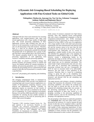
Figure 1 shows the terms that are used throughout this
paper and their definitions. The job grouping and
scheduling algorithm is presented in Figure 2. Figure 3
depicts an example of job grouping and scheduling
scenario where 100 user jobs with small processing
requirements (MI) are grouped into six job groups
according to the processing capabilities (MIPS) of the
available resources and the granularity size.
The overall explanation of Figure 2 is as follows: once
the user jobs are submitted to the broker or scheduler, the
scheduler gathers the characteristics of the available Grid
resources. Then, it selects a particular resource and
multiplies the resource MIPS with the granularity size
where the resulting value indicates the total MI the
resource can process within a specified granularity size.
The scheduler groups the user jobs by accumulating the
MI of each user job while comparing the resulting job
total MI with the resource total MI. If the total MI of user
jobs is more than the resource MI, the very last MI added
to the job total MI will be removed from the job total MI.
Eventually, a new job (job group) of accumulated total
MI will be created with a unique ID and scheduled to be
executed in the selected resource. This process continues
until all the user jobs are grouped into few groups and
assigned to the Grid resources. The scheduler then sends
the job groups to their corresponding resources for further
computation. The Grid resources process the received job
Figure 1: List of terms and their definitions
MI : Million instructions or processing requirements of a user job
MIPS : Million instructions per second or processing capabilities of a resource
Processing Time : Total time taken for executing the user jobs on the Grid
Computation Time : Time taken for computing a job on a Grid resource
JobList : List of user jobs submitted to the broker
RList : List of available Grid resources
JList_Size : Total number of user jobs
RList_Size : Total number of available Grid resources
Job_Listi_MI : MI of ith
user job
RListj_MIPS : MIPS of jth
Grid resource
Granularity_Size : Granularity size (time in seconds) for the job grouping activity
Total_JMI : Total processing requirements (MI) of a job group (in MI)
Total_RMIj : Total processing capabilities (MI) of jth
resource
Total_RMIj = RListj_MIPS *Granularity_Size
GJobList : List of job groups after job grouping activity
TargetRList : List of target resources of each job group
3. groups and send back the computed job groups to the
Grid user. The scheduler then gathers the computed job
groups from the network through its I/O port or queue.
In Figure 3, the granularity size is set to 3 seconds for
example. The scheduler selects a resource of 33 MIPS
and multiply the MIPS with the given granularity size. In
total, that particular resource can process 99 MI of user
jobs within 3 seconds. The scheduler then gathers the user
jobs by accumulating their MI up to 99 MI. In this case,
the first 4 jobs are grouped together resulting in 85 MI.
The fifth job has MI of 22 and grouping of 5 jobs will
results in 107 MI, which is more than the total processing
capability of the selected resource. Once a group of first
four jobs is created, the scheduler assigns a unique ID to
that group. It then selects another resource and performs
the same grouping operations. This process continues
until all the jobs are grouped into a number of groups.
Finally, the scheduler sends the groups to the resource for
job computation.
4 Evaluation
4.1 Implementation with GridSim
GridSim toolkit is used to conduct the simulations based
on the developed scheduling algorithm. Figure 4 depicts
the simulation strategy of the proposed dynamic job
grouping-based scheduler which is implemented using the
GridSim toolkit. The system accepts total number of user
jobs, processing requirements or average MI of those
jobs, allowed deviation percentage of the MI, processing
overhead time of each user job on the Grid, granularity
size of the job grouping activity and the available Grid
resources in the Grid environment (step 1-3). Details of
the available Grid resources are obtained from Grid
Information Service entity that keeps track of the
resources available in the Grid environment. Each Grid
resource is described in terms of their various
characteristics, such as resource ID, name, total number
machines in each resource, total processing elements (PE)
in each machine, MIPS of each PE, and bandwidth speed.
In this simulation, the details of the Grid resources are
-------------------------------------------------------------------------
Algorithm 1.0 Job Grouping and Scheduling Algorithm
-------------------------------------------------------------------------
1 m := 0;
2 for i:= 0 to JobList_Size-1 do
3 for j:=0 to RList_Size-1 do
4 Total_JMI := 0;
5 Total_RMIj :=
RListj_MIPS*Granularity_Size;
6 while Total_JMI Total_RMIj and i
JobList_Size-1 do
7 Total_JMI := Total_JMI + JobListi_MI;
8 i++;
9 endwhile
10 i--;
11 if Total_JMI > Total_RMIj then
12 Total_JMI := Total_JMI – JobListi_MI;
13 i--;
14 endif
15 Create a new job with total MI equals to
Total_JMI;
16 Assign a unique ID for the newly created job;
17 Place the job in GJobListm;
18 Place RListj in TargetRListm;
19 m++;
20 endfor
21 endfor
22 for i:= 0 to GJobList-1 do
23 Send GJobListi to TargetRListi for job
computation;
24 endfor
25 //Job computation at the Grid resources
26 for i:= 0 to GJobList-1 do
27 Receive computed GJobListi from TargetRListi;
28 endfor
Figure 2: Listing of the Job Grouping and Scheduling
Algorithm
Granularity Size: 3 sec
Resource 11/33
Total_RMI: 99
Resource 15/35
Total_RMI: 105
Resource 11/70
Total_RMI: 210
Job 0/20
Job 1/21
Job 2/21
Job 3/23
Job 4/22
Job 5/19
Job 6/18
Job 7/19
Job 8/25
Job 9/28
……….
Job 50/29
Job 51/30
Job 52/29
Job 97/22
Job 98/30
Job 99/24
……….
Job 96/21
Job Group
0/85
Job Group
1/103
Job Group
2/200
Job Group
3/88
Job Group
4/100
Job Group
5/97
User Job ID /
MI
Job Group
ID / MI
Resource
ID/MIPS
Figure 3: An Example of a Job Grouping Strategy
4. Resource MIPS Cost per second
R1 200 100
R2 160 200
R3 210 300
R4 480 210
R5 270 200
R6 390 210
R7 540 320
Table 1: Grid resources setup for the simulation.
store in a file which will be retrieved during the
simulations.
After gathering the details of user jobs and the available
resources, the system randomly creates jobs according to
the given average MI and MI deviation percentage (step
4). The scheduler will then select a resource and multiply
the resource MIPS with the given granularity size (step
5). The jobs will be gathered or grouped according to the
resulting total MI of the resource (step 6), and each
created group will be stored in a list with its associated
resource ID (step 7). Eventually, after grouping all jobs,
the scheduler will submit the job groups to their
corresponding resources for job computation (step 8).
4.2 Experimental Setup
Figure 5 lists the terms used within this section and their
definitions. The inputs to the simulations are total number
of Gridlets, average MI of Gridlets, MI deviation
percentage, granularity size, resource MIPS and Gridlet
processing overhead time.
The tests are conducted using seven resources of different
MIPS, as showed in Table 1.The MIPS of each resource
is computed as follows:
Resource MIPS = Total_PE * PE_MIPS, where
Total_PE = Total number of PEs at the resource,
PE_MIPS = MIPS of PE
Each resource has its own predefined cost rate for
counting the charges imposed on a Grid user for
executing the user jobs at that resource. The MIPS and
cost per second are selected randomly for the simulation
purpose.
In the simulation, the total processing time is calculated
in seconds based on the overhead time for processing
Figure 5: List of terms used within the evaluation and their definition.
(2)
(4)
(3)
(1) JOB SCHEDULER
Grid
resources’
characteristics
Jobs
GRID RES. ID
Grid resource 0
Grid resource 1
Grid resource N
Job MI
Resource MIPS
…Grid resource 0
Job group 0
Grid resource 1
Job group 1 Job group 2
Job groups Resource IDs
Granularity Size
Granularity size
USER JOBS
Total number of jobs
Average MI of job
MI deviation percentage
Overhead processing time
Total MIPS
Grid resource 2
(5)
(6)
(7)
(8)
Figure 4: The simulation strategy for dynamic job grouping-based scheduler
Gridlet : User job
Group : Total number of Gridlet groups created from Gridlet grouping process
R : Resource
A_MI : Average MI rating of Gridlet or Gridlet length in MI
G_Size : Granularity size in seconds
R_MIPS : Resource processing capabilities in MIPS
D_% : MI deviation percentage
OH_Time : Processing overhead time of each Gridlet in seconds
Process_Time : Gridlet processing time in seconds
Process_Cost : Processing cost of the Gridlets
PE : Processing elements in each resource
5. each Gridlets, and the time taken for performing Gridlet
(job) grouping process, sending Gridlets to the resources,
processing the Gridlets at the resources and receiving
back the processed Gridlets. This time computation is
depicted in Figure 6. In real world, the overhead time for
each job depends on the current network load and speed.
In the simulations, the processing overhead time
(OH_Time) of each Gridlet is set to 10 seconds.
The total processing cost is computed based on the actual
CPU time taken for computing the Gridlets at the Grid
resource and at the cost rate specified at the Grid
resource, as summarized below:
Process_Cost = T * C, where
T = Total CPU Time for Gridlet execution, and
C = Cost per second of the resources.
4.3 Experiments, Results and Discussions
4.3.1 Experiment 1: Simulation with and
without Job Grouping
Simulations are conducted to analyse and compare the
differences between two scheduling algorithms: first
come first serve and job grouping-based algorithm
described in section 3 in terms of processing time and
cost. Resources R1 through R4 are used for these
simulations.
Table 2 shows the results of the simulations with and
without job grouping method conducted with granularity
size of 30 seconds and Gridlet average MI of 200. The
simulations managed to execute maximum of 150
Gridlets within 30 seconds. As depicted in Figure 7, the
total processing time and cost are increasing gradually for
simulations without job grouping method compared to
simulations with job grouping method.
When scheduling 25 Gridlets, simulation with job
grouping method groups the Gridlets into one group
according to resource R1’s MI of 6000 (200*30).
Therefore, the total OH_Time is only 10 seconds and the
resulting total Process_Time is 64 seconds. The job
grouping, scheduling and deploying activities take up to
54 seconds. On the other hand, simulation without job
grouping sends all the Gridlets individually to resource
R1 and the total OH_Time is 250 seconds (25*10) leads
to total Process_Time of 280 seconds. In this case, the
total Gridlet computation time (30 seconds) is much less
than the total communication time (250 seconds).Without
grouping, a simulation from 25 to 100 Gridlets yields a
massive increase of 297% in total Process_Time, whereas
simulation with grouping yields only 112.5% rise in
terms of in total Process_Time. As the number of Gridlets
grows, the total Process_Time increases linearly for
simulation without job grouping since total
communication time increased with number of Gridlets.
In simulation with grouping, the communication time
remains constant and major contribution to the total
Process_Time comes from Gridlet computation time at
the resources. With 150 Gridlets, four Gridlet groups are
created, and each resource received one Gridlet group.
Here, 1.48% of the total Process_Time is spent for
communication purpose, whereas in simulation without
grouping, 90.3% of total Process_Time is spent for the
same communication purpose.
Number of
Gridlets
With Grouping Without Grouping
Number of
Groups
Process_Time
(sec)
Process_Cost Process_Time
(sec)
Process _Cost
25 1 64 4979 280 9333
50 2 82 15992 561 38946
75 3 99 35904 838 73485
100 4 136 55332 1112 97741
125 4 186 72332 1388 115673
150 4 270 90124 1662 134843
A_MI:200 D_%:20% G_Size:30 sec R_MIPS: 200,160,210,480 OH_Time:10 sec
Table 2: Simulation with and without job grouping for average MI of 200 and granularity size of 30 seconds
+
+
+
+
Processing overhead time
for Grouped_Gridlet 0
Processing overhead time
for Grouped_Gridlet 1
Processing overhead time
for Grouped_Gridlet 2
Processing overhead time
for Grouped_Gridlet N
Total processing
overhead time
Gridlet Grouping
Time
Time taken to
submit all the
groups to resources
Gridlet Processing
Time
Total processing
time
Time taken to
receive all the
processed Gridlets
Figure 6: Processing time
6. In terms of Process_Cost, the time each Gridlet spends at
the Grid resource is taken into consideration for
computing the total Process_Cost. In simulation with job
grouping, only a small number of Gridlets (Gridlet
groups) are sent to each resource and therefore, the
amount of total overhead time is reduced. In simulation
without job grouping, each small scaled Gridlet sustains a
small amount of overhead time at the Grid resources.
Therefore, the total overhead time incurred by all the
Gridlets at the Grid resource leads to higher processing
cost. For example, when processing 25 Gridlets
individually at the Grid resource, the total Process_Cost
comes up to 9333 units, whereas simulation with job
grouping reduces this cost to 4979 units.
4.3.2 Experiment 2: Simulation of Different
Granularity Sizes with Job Scheduling
Simulations are conducted using different granularity
sizes to examine the total time and cost taken to execute
100 Gridlets on the Grid. Resources R1 through R7 are
used for these simulations.
Table 3 and Figure 8 depict the results gained from
simulations carried out on 100 Gridlets of 200 average
MI using different granularity sizes. Table 4 and Figure 9
show the processing load at each Grid resources when
different granularity sizes are used. The term ‘Gridlet
Computation Time’ in Table 4 refers to the total time
taken for each resource to compute the assigned Gridlet
groups. The communication time is not included in this
computation time.
Job Processing Time for Scheduling with and
without Task Grouping
0
200
400
600
800
1000
1200
1400
1600
1800
25 50 75 100 125 150
User Jobs / Gridlets
ProcessingTime(sec)
With Grouping
Without Grouping
Job Processing Cost for Scheduling with and
without Task Grouping
0
20000
40000
60000
80000
100000
120000
140000
160000
25 50 75 100 125 150
User Jobs / Gridlets
ProcessingCost
With Grouping
Without Grouping
(a) (b)
Figure 7: Processing time (a) and cost (b) for executing 150 Gridlets of 200 average MI within the granularity
size of 30 seconds
Granularity Size (sec) 10 20 30 40 50 60
Process_Time (sec) 160 196 136 120 135 143
Process_Cost 61231 60073 55333 48179 38878 31890
Number of Groups 7 4 4 3 3 2
Gridlets: 100; A_MI:200; D_%:20%; OH_Time:10 sec; Resource: R1-R7
Table 3: Simulation with job grouping for different granularity sizes
Job Processing Time based on Different
Granularity Sizes
0
50
100
150
200
250
10 20 30 40 50 60
Granularity Size (sec)
ProcessingTime(sec)
Time
JobProcessingCost basedonDifferent GranularitySizes
0
10000
20000
30000
40000
50000
60000
70000
10 20 30 40 50 60
Granularity Size (sec)
ProcessingCost
Cost
(a) (b)
Figure 8: (a) Processing time and (b) cost for executing 100 Gridlets of 200 average MI using different granularity sizes
7. From the simulation, it is observed that the total
Process_Time for granularity size of 10 seconds is less
than the one observed for granularity size of 20 seconds.
When granularity size is 10 seconds, 7 job groups are
created (from 100 user jobs) and each resource computes
one job group of almost balanced MI. Since the Gridlet
computations at the Grid resources are done in parallel
and each resource has less processing load (balanced
Gridlet MI), all the Gridlet groups can be computed
rapidly, in 86 minutes.
In the case of granularity size of 20 seconds, four Gridlet
groups are created and 44% of the total Gridlet MI is
scheduled to be computed at resource R4 since it can
support up to 9600 MI. Average Gridlet MI percentage at
the other resources is about 18.7%. Therefore, R4 spent
more time in computing the Gridlet group which leads to
higher total Process_Time.
For granularity size 30 seconds, four Gridlet groups are
produced and resource R3 receives the most MI, about
30.6% of the total MI. The total MI scheduled to all the
resources does not defer much as in the previous case.
Therefore, all the resources can complete the Gridlet
computation in 91 minutes.
The minimum Process_Time is achieved when the
granularity time is 40 seconds. The Gridlet computation
time is same as for the granularity size of 10 seconds, but
less communication time is taken (30 seconds) for dealing
with three Gridlet groups.
In terms of Process_Cost, the resulting cost highly
depends on the cost per second located at each resource
and total Gridlet MI assigned to each resource. In the
simulations, cost per second of using resource R3 (300
units) and R7 (320 units) are more than the other
resources. Therefore, involving these resources in Gridlet
computation will increase the total Process_Cost, e.g. all
the resources are used for Gridlet computation when
granularity size is 10 seconds, which costs 61231 units.
When the granularity size is 20 seconds, R7 is not
engaged in the computation. However, assigning a large
number Gridlet MI (8756 MI) to R4 results in high total
Process_Cost of 60073 units. When the granularity time
is 30 seconds, balanced distribution of the MI among four
resources reduces the total Process_Cost. Another point is
that the total MI assigned to resource R1 is increased as
the granularity size increases. Since R1’s cost per second
is very low (100 units), the total Process_Cost decreases
gradually for granularity sizes 40, 50 and 60 seconds.
From the experiments, it is clear that job grouping
method decreases the total processing time and cost.
However, assigning a large number of Gridlet MI to one
particular resource will increase the total processing time
and cost. Therefore, during the job grouping activity, a
balanced relationship should be determined between total
number of groups to be created from job grouping
Resource/MIPSGranularity
Size (sec) R1/200 R2/160 R3/210 R4/480 R5/270 R6/390 R7/540
Gridlet Computation
Time (sec)
10 1995 1549 2094 4771 2509 3761 3217 86
20 3904 3126 4108 8756 152
30 5809 4775 6094 3217 91
40 7843 6337 5715 86
50 9802 7940 2153 97
60 11898 7997 117
Table 4: Processing load at the grid resources for different granularity sizes
0
2000
4000
6000
8000
10000
12000
Processing
Load (MI)
10 20 30 40 50 60
Granulary Size (sec)
Processing Load at Grid Resources for Different
Granularity Sizes
R1
R2
R3
R4
R5
R6
R7
Figure 9: Processing load at the grid resources for different granularity sizes
8. method, resources’ cost per second, and MI distribution
among the selected resources.
5 Conclusion and Future Work
The job grouping strategy results in increased
performance in terms of low processing time and cost if it
is applied to a Grid application with a large number of
jobs where each user job holds small processing
requirements. Sending/receiving each small job
individually to/from the resources will increase the total
communication time and cost. In addition, the total
processing capabilities of each resource may not be fully
utilized each time the resource receives a small scaled
job. Job grouping strategy aims to reduce the impact of
these drawbacks on the total processing time and cost.
The strategy groups the small scaled user jobs into few
job groups according to the processing capabilities of
available Grid resources. This reduces the communication
overhead time and processing overhead time of each user
job.
Future work would involve developing a more
comprehensive job grouping-based scheduling system
that takes into account QoS (Quality of Service)
requirements as mentioned by Abramson, Buyya, and
Giddy (2002) of each user job before performing the
grouping method. In addition, each resource should be
examined for their current processing load, and jobs
should be grouped according to the available processing
capabilities. Finally, need to consider grouping jobs that
using common data for execution.
6 References
Abramson, D., Buyya, R. and Giddy, J. (2002): A
Computational Economy for Grid Computing, and its
Implementation in the Nimrod-G Resource Broker.
Journal of Future Generation Computer Systems
(FGCS), 18(8): 1061-1074.
Berman, F., Fox, G. and Hey, A. (2003): Grid Computing
– Making the Global Infrastructure a Reality. London,
Wiley.
Buyya, R. and Murshed, M. (2002): GridSim: A Toolkit
for the Modeling, and Simulation of Distributed
Resource Management, and Scheduling for Grid
Computing. Journal of Concurrency and Computation:
Practice and Experience (CCPE), 14(13-15):1175-
1220.
Buyya, R., Date, S., Mizuno-Matsumoto, Y., Venugopal,
S. and Abramson, D. (2004): Neuroscience
Instrumentation and Distributed Analysis of Brain
Activity Data: A Case for eScience on Global Grids.
Journal of Concurrency and Computation: Practice
and Experience, (accepted in Jan. 2004 and in print).
Foster, I. and Kesselman, C. (1999): The Grid: Blueprint
for a New Computing Infrastructure. San Francisco,
Morgan Kaufmann Publisher, Inc.
Gerasoulis, A. and Yang, T. (1992): A comparison of
clustering heuristics for scheduling directed graphs on
multiprocessors. Journal of Parallel and Distributed
Computing, 16(4):276-291.
Gray, J. (2003): Distributed Computing Economics.
Newsletter of the IEEE Task Force on Cluster
Computing, 5(1), July/August.
James, H. A., Hawick, K. A. and Coddington, P. D.
(1999): Scheduling Independent Tasks on
Metacomputing Systems. Proc. of Parallel and
Distributed Computing (PDCS ’99), Fort Lauderdale,
USA.
Logendran, R., Carson, S. and Hanson, E. (2002): Group
Scheduling Problems in Flexible Flow Shops. Proc. of
the Annual Conference of Institute of Industrial
Engineers, USA.
Radulescu, A. and van Gemund, A. (1998): GLB: A
Low-Cost Scheduling Algorithm for Distributed-
Memory Architectures. Proc. of the Fifth International
Conference on High Performance Computing(HiPC
98), Madras, India, pp. 294-301, IEEE Press.
Sarkar, V. (1989): Partitioning and Scheduling Parallel
Programs for Execution on Multiprocessors,
Cambridge, MIT Press.
Yang, T. and Gerasoulis, A. (1994): DSC: Scheduling
Parallel Tasks on an Unbounded Number of
Processors. IEEE Transactions on Parallel and
Distributed Systems, 5(9):951-967.