Incentives and Risk Taking in Hedge Funds *

1. Incentives and Risk Taking in Hedge Funds*
Roy Kouwenberg
†
AEGON Asset Management NL and Erasmus University Rotterdam
William T. Ziemba
‡§
Sauder School of Business, Vancouver and Swiss Banking Institute, University of Zurich
July 17, 2003
*
This research was supported by Inquire Europe.
†
e-mail: kouwenberg@few.eur.nl
‡
Sauder School of Business, University of British Columbia, Vancouver, B.C., Canada,
V6T 1Z2, and Swiss Banking Institute, University of Zurich, Plattenstrasse 14, CH-8032,
Zurich, Switzerland, e-mail: ziemba@interchange.ubc.ca
§
Corresponding author.

2. 1
Incentives and Risk Taking in Hedge Funds
Abstract
This paper presents a theoretical study of how incentives affect hedge fund risk and returns and an
empirical study of the performance of a large group of operating hedge funds. Most hedge fund
managers receive a flat fee plus a share of the returns above a certain benchmark. We investigate
how these features of hedge fund fees affect risk taking by the fund manager in the behavioural
framework of prospect theory. The performance related component encourages funds managers to
take excessive risk. However, risk taking is greatly reduced if a substantial amount of the
manager’s own money is in the fund as well. The empirical results indicate that hedge funds with
incentive fees have higher downside risk than funds without such a compensation contract.
Average returns though, both absolute and risk-adjusted, are significantly lower in the presence of
incentive fees.
JEL Codes: G10, G29
Keywords: hedge funds, incentive fees, optimal portfolio choice

3. 2
As incentive fee arrangements are widespread in the hedge fund industry, it is important to
understand the impact of incentive fees on the investment strategy of hedge fund managers. This
paper presents a theoretical analysis of risk and incentives in the behavioural framework of
prospect theory, followed by an empirical study of risk taking by a large number hedge funds.
Related to our work is a paper by Carpenter (2000) that analyses the effect of incentive fees on
the optimal investment strategy of a fund manager in a continuous-time framework. Carpenter
(2000) finds that a manager with an incentive fee increases the risk of the fund’s investment
strategy if the fund value is below the benchmark specified in the incentive fee contract. This
risk taking behaviour is exactly what one expects, as the fund manager tries to increase the
value of the call option on fund value. If the fund value rises above the benchmark the manager
reduces volatility, in some cases even below the optimal volatility level of a fund without
incentive fees.
We extend the model of Carpenter (2000) along two lines: we incorporate management fees
and investments of the manager in the fund. Most fund managers charge a fixed proportion of
the fund value as management fee, in order to cover expenses and to make a living. One would
expect that management fees moderate risk taking, as negative investment returns will reduce
the future stream of income from management fees. As second important aspect of the hedge
fund industry that affects risk raking, is that most fund managers invest their own money in the
fund. This practice, known as “eating your own cooking”, helps to realign the motivation of the
fund manager with the objectives of the other investors in the fund.
The fact that hedge fund managers typically risk both their career and their own money
while managing a fund is a positive sign to outside investors. The personal involvement of the
manager, combined with a good and verifiable track record, could explain why outside investors
are willing to invest their money in hedge funds, even though investors typically receive very
limited information about hedge fund investment strategies and also possibly face poor liquidity

4. 3
due to lock-up periods. We expect that the hedge fund manager’s own stake in the fund is an
essential factor influencing the relationship between incentives and risk taking.
We analyse the effect of incentive fees on risk taking in a continuous-time framework,
taking management fees and the manager’s own stake in the fund into account. We do not use a
standard normative utility function like HARA for the preferences of the fund manager, but the
behavioural setting of prospect theory instead. Prospect theory is a framework for decision-
making under uncertainty developed by Kahneman and Teversky (1979), based on actual
human behaviour observed in experiments. A number of recent papers argue that prospect
theory is not only relevant for small scale laboratory experiments, but can also help to explain
financial market puzzles, see Benartzi and Thaler (1995), Barberis, Huang and Santos (2001)
and Gomes (2003). Siegmann and Lucas (2002) argue that loss aversion, an important aspect of
prospect theory, can explain the non-normal return distributions of hedge funds. It is therefore
worthwhile to know how hedge fund managers driven by these preferences will react to
incentive fees.
We also derive an expression for the value of the manager’s incentive fee, as in Goetzmann,
Ingersoll, Ross (2003), and show that it can be worth more than 15% of the fund value. We
take into account the fund manager’s optimal investment strategy under prospect theory in
deriving the value of the fee. One of our findings is that loss averse hedge fund managers
increase risk taking in response to the incentive fees, regardless of whether the fund value is
above or below the benchmark. If a substantial amount of the manager’s own money in the fund
(30% or more), risk taking due to incentive fees is reduced considerably. Finally, the value of
the incentive fee option increases enormously as a result of the manager’s optimal investment
strategy, e.g. from 0.8% to 17% of initial fund value.
In the second part of the paper we complement the theoretical analysis with an empirical
study of the risk taking behaviour of a large number of hedge funds in the Zurich Hedge Fund

5. 4
Universe (formerly known as the MAR database). We estimate cross-sectional regressions of
various risk measures on the level of the hedge fund’s incentive fee, controlling for other factors
such as investment style, management fee, size and age. Our analysis is not limited to traditional
risk measures such as volatility, but also includes downside risk, maximum drawdown,
skewness and kurtosis to capture the non-normal shape of hedge fund return distributions. The
empirical relationship between risk taking and incentives in hedge funds has been studied before
by Ackermann, McEnally and Ravenscraft (1999), Brown, Goetzmann and Park (2001),
Agarwal, Daniel and Naik (2002), but all of these papers only consider volatility as a risk
measure, while hedge fund returns are known to be non-normal (Fung and Hsieh 1997, 2001).
The paper is organized as follows. Section I develops a continuous-time framework for
deriving the fund manager’s optimal investment strategy in the framework of prospect theory,
taking into account management fees and the manager’s own investment in the fund.
Subsequently, Section I derives the value of the manager’s incentive fee contract in this setting.
Section II investigates the empirical relationship between risk taking and incentives using a
large database of hedge funds, and Section III concludes.
I. Theoretical Analysis of Incentives and Risk Taking
A. Model Setup
We consider the optimal portfolio problem of a hedge fund manager with initial wealth W(0).
The initial size of the hedge fund is Y(0). The manager owns a fraction of the fund, with 0
1, while outside investors own the remaining portion of the assets (1- ). The management fee
equals a proportion 0 of fund value (1- ) Y(T) at the end of the evaluation period T (i.e. at the
beginning of the next evaluation period). The incentive fee is a percentage 0 of the fund’s
performance in excess of the benchmark B(T) at the end of the evaluation period T:
(1- ) max{ Y(T) - B(T), 0 }. Similar to Carpenter (2000) we assume that the fund manager does

6. 5
not hedge his exposure to the fund’s value with his private portfolio, i.e. his wealth outside of the
fund. For ease of exposition we set the rate of return on the private portfolio equal to the riskless
rate R(0).
1
The portfolio manager’s wealth at the end of the period T is
(1) W(T) = Y(T) + (1 - )Y(T) + (1 - )max{ Y(T) - B(T), 0 } + (1 + R(0))(W(0) - Y(0)) .
The hedge fund manager evaluates wealth at the end of the period T with the value function of
prospect theory (Kahneman and Tverksy 1979)
(2) V(W(T)) = –A ( (T) – W(T) 1
)γ
, if W(T) (T)
( W(T) – (T) 2
)γ
, if W(T) > (T) .
The fund manager has a threshold (T) > 0 for separating gains and losses. The parameters 0 < 1
1 and 0 < 2 1 determine the curvature of the value function over losses and gains
respectively. The parameter A > 0 is the level of loss aversion of the hedge fund manager. In
prospect theory it is assumed that losses loom larger than gains, i.e. A > 1: the pain of a loss
exceeds the positive feeling associated with an equivalent gain.
Risky assets with prices Sk(0) for k = 1, …, K and a riskless asset with price S0(0) are
available as potential investments for the hedge fund manager. The risky asset prices follow Ito
processes with drift rate k(t) and volatility k(t), where t is between 0 and T, while the riskless
asset has a drift rate of r(t) and volatility of zero
(3) dS0(t) = r(t)S0(t)dt
(4) dSk(t) = k(t)Sk(t)dt + k(t)Sk(t)dB(t), k = 1, …, K

7. 6
where the interest rate r(t), the vector of drift rates (t) and the volatility matrix (t) are adapted
processes (possibly path-dependent).
The fund manager selects a dynamic investment strategy, determined by the weights wk(t) of
risky assets k = 1, … , K in the fund, and the weight of the riskless asset w0(t), at any time t in the
continuous interval between 0 and T. For any self-financing vector of portfolio weights w(t) at
time 0 t T, the fund value Y(t) then follows the stochastic process (using vector notation)
(5) dY(t) = r(t)Y(t)dt + ( (t) – r(t))'w(t)Y(t)dt + (t)'w(t)Y(t)dB(t)
where w0(t) = 1 - kwk(t) has been substituted and denotes a (K×1) vector of ones.
The hedge fund manager maximizes the expectation of the value function at the end of the
evaluation period T, by choosing an optimal investment strategy for the fund using
(6) maxw(t) E[V(W(T))]
s.t. W(T) = Y(T) + (1- )Y(T) + (1- )max{ Y(T) - B(T), 0 } + Z(T)
dY(t) = r(t)Y(t)dt + ( (t) – r(t))'w(t)Y(t)dt + (t)'w(t)Y(t)dB(t)
Y(t) 0, for all 0 t T
where Z(T) = (1 + R(0))(W(0) - Y(0)) denotes the fund manager’s wealth outside of the fund at T.
B. The Effect of Incentive Fees on Implicit Loss Aversion
We can analyse the effect of incentive fees on risk taking by examining the value function
V(W(T)) of the fund manager at the end of the evaluation period. Before we proceed with the
analysis we first specify the fund manager personal threshold’s (T), separating gains from losses

8. 7
in the value function. The hedge fund manager will only earn incentives fees if the fund value
Y(T) exceeds the benchmark value B(T) at the end of the evaluation period. Therefore, it seems
plausible that the fund value Y(T) = B(T) is the main point of focus for the manager, separating
failure from success. Just achieving the benchmark B(T) would leave the manager with the
following amount of personal wealth at the end of the year, W(T) = B(T) + (1- )B(T) + Z(T).
We assume that this amount of personal wealth is the threshold that mentally separates gains from
losses for the fund manager
(7) (T) = B(T) + (1- )B(T) + Z(T) .
Given the threshold specification in equation (7), it is easy to demonstrate that the condition
W(T) (T) is equivalent to Y(T) B(T) (see Appendix A for the proof). The manager will
consider fund performance below the benchmark as a loss (failure) and performance in excess of
the benchmark as a gain (success) leading to additional income from incentive fees.
Substituting the expression for W(T) in equation (1) into the value function V(W(T)), yields
(8) V(W(T)) = –A( (T) – ( + (1- )) Y(T) – Z(T) 1
)γ
, if W(T) (T)
( ( + (1- ))Y(T) + (1- )(Y(T) - B(T)) + Z(T) – (T) 2
)γ
, if W(T) > (T) .
Using the fact that W(T) (T) is equivalent to Y(T) B(T) and substituting equation (7) for (T)
into (8) yields the following expression for the manager’s value function
(9) V(W(T)) = –A { ( + (1- ))( B(T) – Y(T) ) 1
}γ
, if Y(T) B(T)
{ ( + ( + )(1- ))( Y(T) – B(T) ) 2
}γ
, if Y(T) > B(T) .

9. 8
We can multiply the value function by a constant, without affecting the solution of the manager’s
optimal portfolio choice problem (6). We simplify the manager’s value function back to the
standard format, multiplying V(W(T)) by ( + ( + )(1- ) 2
) γ
−
(10) V
*
(Y(T)) = –Â ( B(T) – Y(T) 1
)γ
, if Y(T) B(T)
( Y(T) – B(T) 2
)γ
, if Y(T) > B(T)
where  = A ( + (1- ) 1
)γ
⁄ ( + ( + )(1- ) 2
)γ
is the implicit level of loss aversion relevant
for the optimal portfolio choice problem of the fund manager.
Hence, under the relatively mild assumption that the manager’s personal threshold for
separating gains and losses hinges on the hedge fund’s critical level B(T) for earning incentive
fees, the manager’s objective can be reduced back to the standard prospect theory specification in
(10) as a function of fund value Y(T), with B(T) as the threshold separating gains from losses and
 as the implicit level of loss aversion. To investigate the effect of incentive fees on risk taking,
we can now examine the expression for the implicit level of loss aversion  in (11).
Proposition 1: Given 0 < 1, the implicit level of loss aversion  of the hedge fund manager
strictly decreases as a function of the incentive fee , i.e. d ⁄ d < 0.
Proposition 1 shows that an increase in the incentive fee will reduce the implicit level of loss
aversion of the hedge fund manager’s optimal portfolio choice problem. Hence, the manager of a
hedge fund with a large incentive fee should care less about investment losses than a manager
without such a fee, if the fund manager is trying to maximize the expectation of the value
function of prospect theory. Proposition 2 considers the impact of the manager’s own stake in the
fund on the implicit level of loss aversion.

10. 9
Proposition 2: Given 0 1 and > 0, the condition 1 = 2 is sufficient for a strictly positive
relation between the manager’s own stake in the fund and the implicit level of loss aversion Â,
i.e. d ⁄ d > 0.
Given 1 = 2, Proposition 2 states that a manager with a large own stake in the fund should
optimally care more about losses than a manager without such a stake. The sufficient condition
1 = 2 means that the value function has the same curvature over gains as over losses. Tversky
and Kahneman (1992) have estimated the parameters of the value function of prospect theory
from the observed decisions made under uncertainty by a large group of people. The estimates of
Tversky and Kahneman (1992) are A = 2.25 for the average level of loss aversion and 1 = 2 =
0.88 for the curvature of the value function. As Tversky and Kahneman (1992) did not find a
significant difference between 1 and 2, the condition 1 = 2 of Proposition 2 seems plausible.
Given these estimated preference parameters, Figure 1 displays the implicit level of loss
aversion  as a function of the incentive fee for three different levels of the manager’s stake in the
fund ( = 5%, = 20% and = 50%). Figure 1 demonstrates that the manager’s implicit level of
loss aversion is equal to 2.25 without incentive fees ( = 0). As the incentive fee increases, the
implicit level of loss aversion of the fund manager starts to decrease, indicating that the manager
should optimally care less about losses and more about gains due to the convex compensation
structure. The negative impact of incentive fees on implicit loss aversion is mitigated to some
extent if the manager owns a substantial part the fund.
C. The Optimal Investment Strategy with Incentive Fees
We will now derive the optimal dynamic investment strategy of the fund manager. In the
previous section we reduced the value function of the fund manager back to standard format

11. 10
V
*
(Y(T)), as a function of terminal fund value Y(T). Hence, the optimal portfolio choice problem
(6) is equivalent to
(11) maxw(t) E[V
*
(Y(T))]
s.t. dY(t) = r(t)Y(t)dt + ( (t) – r(t))'w(t)Y(t)dt + (t)'w(t)Y(t)dB(t)
Y(t) 0, for all 0 t T .
To facilitate the solution of the optimal portfolio choice problem we assume that markets are
dynamically complete. Market completeness implies the existence of a unique state price density
(t), also known as pricing kernel, defined as
(12) d (t) = - r(t) (t)dt - κ(t) (t)dB(t), (0) = 1
where (t) = (t)
-1
(t)( (t) – r(t)) denotes the market price of risk.
Under the assumption of complete markets, Berkelaar, Kouwenberg and Post (2003) solve the
optimal portfolio choice problem of a loss averse investor in (6) with the martingale
methodology, following Basak and Shapiro (2001). The solution is derived in two steps. First, the
optimal fund value Y
*
(T) is derived as a function of the pricing kernel (T) at the planning horizon
(see Proposition 3). Second, the optimal dynamic investment strategy that replicates these fund
values is derived under the assumption that the risky asset prices follow Geometric Brownian
motions and the riskless rate is constant (see Proposition 4). See Berkelaar, Kouwenberg and Post
(2003) for more details and proofs.
Proposition 3: Under the assumption of a complete market, the optimal fund value Y
*
(T) for the
manager at the evaluation period T, as a function of the pricing kernel, is

12. 11
(13) Y
*
(T) = B(T) +
)
1
2
/(
1
2
)
(
−
γ
γ
ξ T
y
, if (T) <
*
0 , if (T)
*
where
*
solves f( ) = 0 with
(14) f(x) = B(T) +
)
2
1
/(
1
2
)
2
1
/(
2
2
2
)
(
1
1 γ
γ
γ
γ
γ
γ −
−
−
yx
– B(T)yx + ÂB(T)
2
and y 0 satisfies E[ (T)Y(T) ] = (0)Y(0).
Proposition 4: Under the assumption of a complete market, Geometric Brownian motions for the
risky asset prices and a constant interest rate r(t)=r0, the optimal dynamic investment strategy
w
*
(t) of the fund manager as a function of the pricing kernel (t) and fund value Y(t) is
(15) w
*
(t)=
−
+
−
+
−
′ Γ
−
−
−
−
2
*
2
*
2
)
(
)
1
/(
1
2
*
1
)
(
1
1
)
(
(
)
(
)
(
(
)
(
)
(
))
(
(
)
(
)
(
)
(
2
γ
ξ
κ
ξ
φ
ξ
γ
κ
ξ
φ
κ
σ
γ
d
N
t
T
d
e
t
y
t
T
d
e
t
B
t
Y
t
t
T
r
(16) Y(t) = ))
(
(
)
(
))
(
(
)
( *
2
)
(
)
2
1
/(
1
2
*
1
)
(
ξ
ξ
γ
ξ
γ
d
N
e
t
y
d
N
e
t
B t
t
T
r Γ
−
−
−
+
(17) (t) = )
(
1
2
1
)
(
2
1
1 2
2
2
2
2
2
2
t
T
t
T
r −
−
+
−
+
−
κ
γ
γ
κ
γ
γ
(18)
t
T
t
T
r
t
x
x
d
−
−
−
+
=
κ
κ
ξ )
)(
5
.
0
(
))
(
/
log(
)
(
2
1 and
2
1
2
1
)
(
)
(
γ
κ
−
−
+
=
t
T
x
d
x
d .
where N(·) is the standard normal cumulative distribution and φ (·) is the density function.
To analyze the effect of incentive fees on the investment strategy of the fund manager, we can
use the fact that the implicit level of loss aversion  of the fund manager decreases as a function
of the incentive fee level (see Proposition 1). The next proposition shows how a decrease of Â

13. 12
affects the optimal fund values Y
*
(T) at the evaluation date T.
Proposition 5: Given 0 < 1, an increase of the hedge fund manager’s incentive fee will lead
to a decrease in the breakpoint
*
of the optimal fund value function Y
*
(T) and a decrease of the
Lagrange multiplier y.
Proposition 5 shows that an increase of the incentive fee makes the manager seek more payoffs in
good states of the world with low pricing kernel (due to the decrease of y) and less in bad states
(due to the decrease of
*
).
The effect of an increase of the incentive fee on the optimal investment strategy is illustrated
in Figure 2. For ease of exposition, we assume that there is only one risky asset, representing
equity, with a Sharpe ratio of = 0.10 and a volatility of = 20%, and a riskless asset with r0 =
4%. The evaluation period is one year (T = 1) and the fund manager has the standard preference
parameters for the value function (A = 2.25, 1 = 2 = 0.88). The initial fund value is Y(0) = 1, the
threshold for the incentive fee is B(T) = 1, the management fee is = 1% and the manager’s own
stake in the fund is = 20%. Given these parameters, Figure 2 shows the optimal weight of risky
assets in the fund w
*
(t), as a function of fund value Y(t) at time t = 0.5. Each line in Figure 2
represents a different level of incentive fee , ranging from 0% to 30%.
Figure 2 shows that the fund manager takes more risk in response to an increasing incentive
fee. The increase in risk is more pronounced when fund value drops below the benchmark B(T).
Due to the structure of the value function of prospect theory, a fund manager without an incentive
fee will increase risk at low fund values as well; incentive fees amplify this behaviour. Figure 3
shows the effect on the optimal investment strategy of changing the manager’s own stake in the
fund , given an incentive fee of = 20%. Figure 3 demonstrates that an increase of the
manager’s share in the fund can completely change risk taking. With a stake of 10% or less, the

14. 13
manager behaves extremely risk seeking as a result of the incentive fee. However, with a stake of
30% or more, the investment strategy is very similar to the base case of 100% ownership (without
an incentive fee). Finally, Figure 4 shows the manager’s initial weight of risky assets w(0), as a
function of the incentive fee . The different lines in Figure 4 represent different levels of the
manager’s own stake in the fund ( ). Again higher incentive fees lead to increased risk taking; the
increase in risk taking is more drastic when the managers own stake in the fund is low ( 30%).
D. The Value of the Manager’s Incentive Fee Option
A typical hedge fund charges a fixed fee of 1% to 2% and an incentive fee of 20%. For hedge
fund investors it is worthwhile to know what the value of these fee arrangements is. We can use
the framework developed to determine the option value of hedge fund fees. In a complete market,
any European option with a set of payoffs X(T) at time T can be priced as follows with the pricing
kernel (T)
(19) X(0) = (0)
-1
E[ (T)X(T) ]
where X(0) is the initial value of the contingent claim. The pay off of the incentive fee at time T
under the manager’s optimal strategy is X(T) = max{ Y
*
(T) – B(T), 0 }. Hence, we can find the
value of the incentive fee at time 0 by calculating the expectation in (19).
Proposition 6: Under the assumption of a complete market, Geometric Brownian motions for the
risky asset prices and a constant interest rate r(t)=r0, the initial value of the incentive fee X(0),
given the fund manager’s optimal investment strategy, is
(20) X(0) = ))
(
(
)
0
(
*
2
)
0
(
)
2
1
/(
1
2
ξ
ξ
γ Γ
γ
d
N
e
y
−

15. 14
(21) (0) = T
T
r 2
2
2
2
2
2
2 1
2
1
2
1
1
κ
γ
γ
κ
γ
γ −
+
+
−
(22)
T
T
r
x
x
d
κ
κ
ξ )
5
.
0
(
))
0
(
/
ln(
)
(
2
1
−
+
= and
2
1
2
1
)
(
)
(
γ
κ
−
+
=
T
x
d
x
d .
where N(·) is the standard normal cumulative distribution.
Figure 5 plots the value of a 20% incentive fee as a function of the manager’s stake in the
fund, using the same set of parameters as in Figure 2 ( = 0.10, = 20%, r0 = 4%, T = 1, Y(0) = 1,
B(T) = 1, = 1% and A = 2.25, 1 = 2 = 0.88). Figure 5 shows that the value of the 20% incentive
fee ranges from 0.8% to 17% of the initial fund value, depending on the manager’s own stake in
the fund. If the manager’s stake in the fund is 100%, the manager does not care about the
incentive fee and manages the fund conservatively since it is a personal account. However, as the
manager’s stake in the fund goes to zero, the manager starts to increase the volatility of the
investment strategy in order to reap more profits from the incentive fee contract. Figure 6 shows
the optimal volatility of the fund returns Y(T)/Y(0) as a function of the manager’s stake in the
fund, given the incentive fee of 20%. Figure 6 shows that the fund manager greatly increases the
fund’s return volatility as the manager’s own stake in the fund decreases, in order to maximize the
expected payoff of the incentive fee. The increase of the value of the incentive fee due to this
change in investment behaviour is as much 2125% in this example (namely, from 0.8% to 17% of
initial fund value).
E. Other Factors Influencing Incentives and Risk Taking in the Hedge Fund Industry
We would like to point out a number of other aspects of the hedge fund industry that have not
been embedded in our theoretical model, but that also affect the relationship between incentives
and risk taking. Many incentive fee arrangements in the hedge fund industry include a high-water
mark provision, stating that losses from previous periods should be made up before any incentive

16. 15
fees will be paid. The effect of high-water marks on risk taking is two-fold. First, if the fund value
is below the benchmark of the incentive fee arrangement at the end of the current evaluation
period, then the incentive fee option of a fund manager with a high-water mark will be ‘out-of-
the-money’ at the start of the next evaluation period. The optimal response of the fund manager to
this situation is to start the new evaluation period with a relatively risky investment strategy (see
Figure 2).
The second effect of a high-water mark provision is that it leads to a concave relationship
between fund value and the value of future incentive fee payments, which reduces risk taking. To
explain this effect, consider the strike price of the new incentive fee option issued at the
beginning of the next evaluation period (at time T). In case of losses (Y(T) < B(T)), the new option
will get strike price B(T) due to the high-water mark provision, and it will lose value rapidly as
Y(T) drops further below B(T). With gains (Y(T) > B(T)), the strike price of the new option is
adjusted upward, which puts a drag on the increase of the option value as a function of Y(T). The
result is a concave relation between fund value and the value of the new incentive fee option,
reducing the manager’s implicit level of loss aversion.
Whether high-water marks will eventually increase or decrease risk taking depends on many
parameters, such as the manager’s trade-off between current wealth and future wealth, and the
hurdle rate used for setting the benchmark B(T). An analytical study of the overall effect of high-
water marks on risk taking requires a framework with at least two performance evaluation
periods, in order to model the relationship between the manager’s current choices and the future
payoff of the incentive fee contract. Adding a second evaluation period to our continuous-time
framework will render the model analytically intractable, due to the complexity of the optimal
fund value process (16). Goetzmann, Ingersoll and Ross (2003) analyze the effect of high-water
marks analytically, however in their framework the investment strategy of the fund manager is
fixed (not optimized) and fees are earned continuously instead of periodically.

17. 16
Fund flows are another important factor affecting risk taking in a multi-period setting.
Agarwal, Daniel and Naik (2002) find that the relationship between hedge fund performance and
subsequent fund flows is convex, just like in the mutual fund industry (Chevalier and Ellison
1997, Sirri and Tufano 1998). Outperforming hedge funds attract significant amounts of new
money, while withdrawals after poor performance are relatively small. The convex flow-
performance relation creates an incentive for fund managers to increase risk taking, especially
after poor performance. Other aspects that might affect risk taking are peer group pressure and the
expectations of investors about the appropriate risk level of hedge funds. For example, hedge
funds within the market-neutral style group have on average displayed relatively low return
volatility in the past. Therefore, a market-neutral hedge fund with highly volatile returns will
probably be looked upon rather suspiciously by investors, as the fund does not conform to the
characteristic of its peer group. Increased risk taking could therefore lead to fund outflows
(Agarwal, Daniel and Naik 2002 report evidence for this relationship).
All in all, the number of factors that can influence the relationship between risk taking and
incentives in the hedge fund industry is rather overwhelming. It is not the aim of this paper to
include every aspect of the hedge fund industry in a theoretical analysis of risk taking and
incentives, as the model is intended to be a simplified image of reality, and not reality itself.
Instead, in the next section we proceed with an empirical investigation, in order to see whether
hedge funds with incentive fees indeed take on more risk than funds without such an
arrangement.
II. Empirical Analysis of Incentives and Risk Taking in Hedge Funds
A. Hedge Fund Data
For our empirical investigation we use the Zurich Hedge Fund Universe, formerly known
as the MAR hedge fund database, provided by Zurich Capital Markets. The database includes

18. 17
a large number of funds that have disappeared over the years, which reduces the impact of
survivorship bias. The data starts in January 1977 and ends in November 2000. Overall there
are 2078 hedge funds in the database and 536 fund of funds. We will analyse the hedge fund
data from January 1995 to November 2000 since the database keeps track of funds that
disappear starting January 1995. The return data is net of management fees and net of
incentive fees.
The hedge funds in the database are classified into eight different investment styles by the
provider: Event-Driven, Market Neutral, Global Macro, Global International, Global Emerging,
Global Established, Sector and Short-Sellers. We will merge the styles Global International,
Global Established and Global Macro into one group, denoted Global Funds, as these three styles
have similar investment style descriptions. We treat the Global Emerging funds as a separate
category, denoted Emerging Markets, as the funds within this style are often unable to short
securities and emerging market funds have quite different return characteristics compared to the
other global funds.
Table 1 provides some descriptive statistics of the funds in the database. The table
distinguishes between funds that were still in the database in November 2000 (alive) and funds
that dropped out (dead) and between individual hedge funds and fund of funds. The median
incentive fee for hedge funds is 20%. An incentive fee of 20% seems to be the industry standard,
as 71.4% of the funds use it. Only 8.5% of all hedge funds do not charge an incentive fee. The
median management fee is 1%. The majority of funds (71.5%) charge a fee between 0.5% and
1.5%, while only 4.2% of the funds do not charge a management fee. On top of this, an investor
in fund of funds has to pay fees to the fund of fund manager. On average fund of funds charge
slightly lower fees than individual hedge funds, although the median incentive fee is still 20%
(dead and alive funds combined). Only 6.2% of fund of funds do not charge an incentive fee. The
median management fee of fund of funds is 1%. The funds in the database are relatively young,

19. 18
with an average age of 4 years for living funds and 2.6 years for dead funds (same for hedge funds
and fund of funds). The relatively young age of the funds has to do with the rapid growth of the
hedge fund industry over the period 1995-2000. For a study of the performance of the funds in the
database over this period see Kouwenberg (2003).
B. Incentives and Risk Taking in Hedge Funds: Empirical Results
Empirical studies of incentives and risk taking in the literature typically test whether funds
with poor performance in the first half of the year increase risk in the second half of the year, (see
e.g.. Brown, Harlow and Starks 1996, Chevalier and Ellison 1997 and Brown, Goetzmann and
Park 2001). The idea behind this approach is that funds with an incentive fee, or facing a convex
performance-flow relationship, will increase risk after bad performance in the first half of the year
in order to increase the value of their out-of-the-money call option on fund value. Considered
within the context of the prospect theory framework applied in this paper, such a test is less
meaningful. Loss averse fund managers will always increase risk as their wealth drops below the
threshold, regardless of incentive fees (see Figure 2). A more distinguishing effect of incentive
fees within the prospect theory framework is that incentives reduce implicit loss aversion and lead
to increased risk taking across the board, even at the start of the evaluation period (see Figure 4).
We will therefore test if the risk of hedge funds returns increases as a function of the fund’s
incentive fee.
Hedge fund returns are well known to be non-normal due to the dynamic investment
strategies of the funds (see Fung and Hsieh 1997, 2001 and Mitchell and Pulvino 2001). Still,
empirical studies of the relationship between risk taking and incentives in hedge funds only
consider volatility as a risk measure (Ackermann, McEnally and Ravenscraft 1999, Brown,
Goetzmann and Park 2001 and Agarwal, Daniel and Naik 2002), even though volatility can not
fully capture the non-normal shape of hedge fund return distributions. To address this problem,

20. 19
we will focus on non-symmetrical risk measures, namely the 1
st
downside moment and
maximum drawdown, as well as the skewness and kurtosis of hedge fund returns. The 1
st
downside (upside) moment is defined as the conditional expectation of the fund returns below
(above) the risk free rate. Maximum drawdown is defined as the worst performance among all
runs of consecutive negative returns.
Table 2 shows the cross-sectional average of ten different risk and return measures of the
hedge funds in the database, conditional on the level of the incentive fee. The risk measures are
volatility, 1
st
downside moment (relative to the risk free rate), maximum drawdown, skewness
and kurtosis. The return measures are the fund’s mean return and 1
st
upside moment. Finally,
Table 2 lists three risk-adjusted performance measures, namely the Sharpe ratio, Jensen’s alpha
and the gain-loss ratio. The gain-loss ratio is defined as the ratio of the 1
st
upside moment to the
1
st
downside moment. Berkelaar, Kouwenberg and Post (2003) demonstrate that the gain-loss
ratio can be interpreted as a measure of the investor’s implicit level of loss aversion. The last
column of Table 2 displays the p-value of an ANOVA-test for differences in means between the
incentive fee groups.
The first row of Table 2 shows that hedge funds without incentive fee, on average, have
considerably higher mean returns than funds that do charge an incentive fee (means are
significantly different between groups). Apparently funds with an incentive fee cannot make up
for the costs of the fee. We do not find statistically significant evidence that incentive fees lead to
drastic changes in average volatility, 1
st
downside moment and maximum drawdown of hedge
funds. We do find significant differences in average skewness and kurtosis between incentive fee
groups. However, the latter finding seems to be caused mainly by the relatively small group of
funds with an incentive fee in excess of 20%.
When we examine the results for the three risk-adjusted performance measures, Sharpe ratio,
alpha and gain-loss ratio, we find significant differences between incentive fee groups. Funds

21. 20
without an incentive fee achieve the best risk-adjusted performance on average, while funds
charging a below average incentive fee have relatively poor performance. Overall, we conclude
from Table 2 that incentive fees reduce the mean return and risk-adjusted performance of funds,
while the effects on risk are not very clear-cut. We have also analysed the data after correcting for
differences in investment styles by measuring deviations from the average in each style group, but
the conclusions do not change materially (results available on request from the authors).
To control for other hedge fund characteristics such as fund size, age, management fee and
investment style group, we also estimate the following cross-sectional regression model for the
hedge fund risk and return measures
(23) ai = =
H
h ih
d
1 + ifi + mfi + navi + agei + i ,
with i = 1, …, I and i ~ N(0, ) independently normally distributed,
where ai denotes the cross-sectional hedge fund statistic under consideration of fund i = 1, …, I,
dih is a dummy which equals one if fund i belongs to hedge fund style h = 1, ..., H and zero
otherwise, ifi is the incentive fee, mfi the management fee, navi is the mean net asset value of the
fund and agei is the number of years that the fund is in the database.
Table 3 reports the cross-sectional regression results. Columns 2 to 6 in Table 3, denoted by
Regression A, refer to regression model (23) above; columns 7 to 11, denoted by Regression B,
refer to a slightly modified version of the model, which uses a dummy variable for the incentive
fee and a dummy for the management fee; the dummy variables are one if a fee is charged and
zero otherwise. We do not report the estimated hedge fund style dummies dih in Table 3 to save
space. If we concentrate on the results for the incentive fee variable in Table 3, we find that funds
with higher fees earn significantly lower mean returns. The only other significant effect of
incentive fees is a reduction of Sharpe ratios and alphas (only in Regression B, with incentive fee

22. 21
dummies). There is no significant effect of incentive fees on any of the five risk measures at the
5% confidence level. However, we do see an economically relevant increase of the 1
st
downside
moment and the maximum drawdown due to incentive fees, as the estimated coefficients are quite
substantial. Moreover, the increase in the 1
st
downside moment is significant at the 10% level in
both regressions. We conclude that there is some evidence for increased risk taking due to
incentive fees if we focus on downside risk instead of volatility as a risk measure.
C. Incentives and Risk Taking in Fund of Funds: Empirical Results
We now repeat the empirical analysis for the fund of funds in the database. Table 4 displays
the cross-sectional average of the ten risk and return measures, conditional on the level of the
incentive fee. We use three incentive fee groups instead of four, due to the relatively small
number of fund of funds (403 in total). Again we find significant differences between the average
mean returns of the incentive fee groups. Fund of funds with high fees earn higher returns on
average. The 1
st
upside moment is also significantly different across groups and larger for fund of
funds with fatter fees. We do not find significant differences in the five risk measures between
groups. The three risk-adjusted performance measures, Sharpe ratio, alpha and gain-loss ratio, are
significantly different across groups and relatively large for fund of funds with high fees ( 20%).
Table 5 contains the estimation results of the cross-sectional regression model (23) for fund of
funds.
2
The coefficient of the incentive fee variable is significantly positive in the cross-sectional
regression on the 1
st
upside moment, volatility, maximum drawdown and gain-loss ratio (at the
5% level). There is an economically relevant positive impact on the mean return, 1
st
downside
moment, skewness and Sharpe ratio as well, based on the magnitude of the estimated coefficients.
Hence, for the fund of funds in the database we find that higher incentive fees are linked to
increased upside potential and increased risk taking. Risk-adjusted returns increase as well, so
investors seem to be better of with fund of funds that charge higher incentive fees. In the case of

23. 22
management fees, Table 5 shows that they are a drag on performance: higher fees significantly
reduce average returns, Sharpe ratios and alphas.
A potential explanation for the positive relationship between incentive fees and (risk-adjusted)
returns in Table 4 and 5 might be that fund of fund managers with incentive fees opt for a more
risky basket of hedge funds to increase the value of their call option on fund value, leading to
more upside return potential and more risk as well. The fund of fund managers themselves might
argue that funds with better manager selection skills generate higher returns and are therefore able
to charge higher incentive fees. A weak point of the latter story is that it does not explain why
fund of fund managers with better skills have more risky returns on average as well; the skill
advantage should allow good managers to achieve better returns, while taking less risk.

24. 23
III. Conclusions
In this paper we analyse the relationship between incentives and risk taking in the hedge
fund industry. We use prospect theory to model the hedge fund manager’s behaviour and derive
the optimal investment strategy for a manager in charge of a fund with an incentive fee
arrangement. We find that incentive fees reduce the manager’s implicit level of loss aversion,
leading to increased risk taking. However, if the manager’s own stake in the fund is substantial
(e.g. > 30%), risk taking will be reduced considerably. We also derive an expression for the
option value of the incentive fee arrangement, taking into account the manager’s optimal
investment strategy. We show that the fund manager increases the value of the incentive option
by increasing the volatility of fund returns.
In the second part of the paper we examine empirically whether hedge fund managers with
incentive fees indeed take more risk in practice, using the Zurich Hedge Fund Universe
(formerly known as the MAR database) in the period January 1995 to November 2000. The
cross-sectional analysis mainly shows that hedge funds with incentive fees have significantly
lower mean returns (net of fees) and worse risk-adjusted performance. There is no significant
effect on volatility, but the 1
st
downside moment of returns increases substantially in the
presence of incentive fees (significant at the 10% level). Our results illustrate the importance of
using downside risk measures, given the non-normality of hedge funds returns.
Funds of funds charging higher incentive fees have more risky and higher returns on
average. Hence, it seems that fund of funds take more risk in response to incentive fees. It seems
unlikely that fund of fund managers with higher incentive fees are more skilful, as that story
does not explain why risk taking increases as well as a function of incentive fees.

25. 24
REFERENCES
Ackermann, C., McEnally, R. and D. Ravenscraft, 1999, The Performance of Hedge Funds:
Risk, Return and Incentives, Journal of Finance, vol. 54, 833-874.
Agarwal, V., Daniel, N.D. and N.Y. Naik, 2002, Determinants of Money-Flow and Risk-taking
Behavior in the Hegde Fund Industry, Working paper, London Business School.
Barberis, N., Huang, M. and Santos, T, 2001, Prospect Theory and Asset Prices, Quarterly
Journal of Economics, vol. 116, 1-53.
Basak, S., Pavlova, A. and A. Shapiro, 2003, Offsetting the Incentives: Risk Shifting, and
Benefits of Benchmarking in Money Management, Working paper, MIT.
Basak, S. and A Shapiro, 2001, Value-at-Risk Based Risk Management: Optimal Policies and
Asset Prices, Review of Financial Studies, vol. 14, 371-405.
Benartzi, S. and Thaler, R., 1995, Myopic Loss Aversion and the Equity Premium Puzzle,
Quarterly Journal of Economics, vol. 110, 73-92.
Berkelaar, A.B., Kouwenberg, R. and G.T. Post, 2003, Optimal Portfolio Choice under Loss
Aversion, Working paper, Erasmus University Rotterdam.
Brown, K.C., Harlow, W.V. and L.T. Starks, 1996, Of Tournaments and Temptations: An
Analysis of Managerial Incentives in the Mutual Fund Industry, Journal of Finance,
vol. 51, 85-109.
Brown, S.J., Goetzman, W.N. and J. Park, 2001, Careers and Survival: Competition and Risk in
the Hedge Fund and CTA Industry, Journal of Finance, vol. 56, 1869-1886.
Carpenter, J., 2000, Does Option Compensation Increase Managerial Risk Appetite?, Journal of
Finance, vol. 55, 2311-2331.
Chevalier. J. and G. Ellison, 1997, Risk Taking by Mutual Funds as a Response to Incentives,
Journal of Political Economy, vol. 105, 1167-1200.

26. 25
Elton, J.E., Gruber, M.J., and C.R. Blake, 2003, Incentive Fees and Mutual Funds, Journal of
Finance, vol. 58, 779-804.
Fung, W. and D.A. Hsieh, 1997, Empirical Characteristics of Dynamic Trading Strategies: The
Case of Hedge Funds, Review of Financial Studies, vol. 10, 275-302.
Fung, W. and D.A. Hsieh, 2001, The Risk in Hedge Fund Strategies: Theory and Evidence from
Trend Followers, Review of Financial Studies, vol. 14, 313-341.
Goetzmann, W.N., Ingersoll, J.E. and S.A. Ross, 2003, High-Water Marks and Hedge Fund
Management Contracts, Journal of Finance, forthcoming.
Gomes, F., 2000, Portfolio Choice and Trading Volume with Loss Averse Investors, Journal of
Business, forthcoming.
Kahneman, D.H. and A. Tversky, 1979, Prospect Theory: An Analysis of Decision Making
under Risk, Econometrica, vol. 47, 263-290.
Kouwenberg, R., 2003, Do Hedge Funds Add Value to a Passive Portfolio: Correcting for Non-
Normal Returns and Disappearing Funds, Journal of Asset Management, vol. 3, 361-382.
Mitchell, M. and T. Pulvino, 2001, Characteristics of Risk and Return in Risk Arbitrage,
Journal of Finance, vol. 56, 2135-2175.
Siegmann, A. and A. Lucas, 2002, Explaining Hedge Fund Investment Styles by Loss Aversion,
Working paper, Vrije Universiteit Amsterdam.
Sirri, E.R. and P. Tufano, 1998, Costly Search and Mutual Fund Flows, Journal of Finance,
vol. 53, 1589-1622.
Tversky, A. and D.H. Kahneman, 1992, Advances in Prospect Theory: Cumulative
Representation of Uncertainty, Journal of Risk and Uncertainty, vol. 5, 297-323.

27. 26
APPENDIX A
Proof of the equivalence of W(T) (T) and Y(T) B(T)
Substituting (1) for W(T) and (7) for (T), W(T) (T) is equivalent to
(A1) Y(T) + (1 - )Y(T) + (1 - )max{ Y(T) - B(T), 0 } + Z(T) B(T) + (1- )B(T) + Z(T).
Rearranging terms to the left-hand-side, it follows that (A1) is equivalent to (A2)
(A2) (Y(T)- B(T)) + (1 - ) (Y(T)- B(T)) + (1 - )max{ Y(T) - B(T), 0 } 0.
Finally, it is easy to see that (A2) holds if and only if Y(T) B(T).
Proof of Proposition 1
The manager’s implicit level of loss aversion is
(A3) Â = A ( + (1- ) 1
)γ
⁄ ( + ( + )(1- ) 2
)γ
.
Differentiating  with respect to yields
(A4) d / d = - 2(1- ) A ( + (1- ) 1
)γ
⁄ ( + ( + )(1- ) 1
2
) +
γ
.
Given 0 < 1, A > 0, 0, 0 and 0 < 2 1, the inequality d / d < 0 holds.

28. 27
Proof of Proposition 2
The manager’s implicit level of loss aversion is given in (A3).
Differentiating  with respect to yields
(A5) d / d =  ( 1(1- )( + (1- ))
-1
- 2(1- - )( + ( + )(1- ))
-1
) .
Note that d / d > 0 is equivalent to
(A6) 1(1- )( + ( + )(1- )) > 2(1- - )( + (1- )) .
Given 0 < 1, 0, > 0, the condition 1 = 2 is sufficient for d / d > 0.
Proof of Proposition 3
See Berkelaar, Post and Kouwenberg (2003).
Proof of Proposition 4
See Berkelaar, Post and Kouwenberg (2003).
Proof of Proposition 5
An increase of the manager’s incentive fee leads to a reduction of the implicit level of loss
aversion  (see Proposition 1). Berkelaar, Post and Kouwenberg (2003) prove that a decrease of Â
leads to a decrease in the breakpoint
*
of the optimal fund value function Y
*
(T) and a decrease of
the Lagrange multiplier y.

29. 28
Proof of Proposition 6
We substitute the pay off of the incentive fee contract X(T) into equation (19) to yield (A7):
(A7) X(0) = (0)
-1
E[ (T) max{ Y
*
(T) – B(T), 0 } ]
Equation (A7) can be simplified by substituting the manager’s optimal fund value function Y
*
(T)
(A8) X(0) = )
(
)
(
)
(
*
0
)
1
2
/(
1
2
T
d
T
y
T ξ
γ
ξ
β
ξ
ξ γ −
.
Under the assumption of a complete market, a constant risk free rate and Geometric Brownian
motions for the asset prices, the pricing kernel (T) at time T is log-normally distributed. Using
this fact, the expression in (20) for X(0) follows from solving the integral (A8).

30. 29
Table 1 Characteristics of the hedge fund data
Descriptive statistics of the hedge funds in the database from January 1995 to November 2000 are
displayed. The cross-sectional mean, median and standard deviation of the incentive fee, the management
fee, the net asset value and the age of the fund are listed respectively. Alive funds were still in the
database in November 2000, while dead funds dropped out before this date. We exclude funds that do not
report fees.
Hedge funds Fund of funds
Alive Dead Alive Dead
Incentive fee Mean
Median
Std. Dev.
18.2
20.0
6.2
17.9
20.0
7.0
16.7
20.0
5.2
13.5
15.0
7.4
Management fee Mean
Median
Std. Dev.
1.22
1.00
0.52
1.30
1.00
0.64
1.04
1.20
0.75
1.12
1.00
0.70
Net Asset Value Mean
Median
Std. Dev.
2,361
1,190
9,941
2,260
1,015
11,107
1,319
1,121
2,438
1,004
158
21,254
Age (years) Mean
Median
Std. Dev.
3.81
3.92
1.81
2.64
2.42
1.60
4.17
4.58
1.85
2.58
2.42
1.53
Number of funds 772 470 307 144

31. 30
Table 2 Hedge fund risk and returns conditional on incentive fee
The average cross-sectional risk and returns of the hedge funds in the database from January 1995 to
November 2000 are displayed, conditional on the incentive fee charged by the fund. The sample includes
both funds that were still in the database in November 2000 and funds that dropped out before this date.
Only funds with at least 12 monthly observations are included. The last column denotes the p-value of an
ANOVA-test for equality of the means of the four incentive fee groups.
†
As outliers influence the mean of
the gain-loss ratio heavily, we use the median instead and report the p-value of the Kruksal-Wallis test for
differences in the median in the last column.
Overall Mean conditional on incentive fee
mean if=0 0<if<20 if=20 if >20 p-value
Average return 15.4 23.7 13.3 15.2 11.8 0.0%
1
st
Upside moment 30.6 37.1 31.2 30.4 23.2 0.4%
Volatility 20.0 21.4 21.0 19.8 17.9 45.6%
1
st
Downside moment 20.2 18.4 23.0 20.2 16.5 16.3%
Maximum drawdown 23.0 19.4 26.4 22.8 22.9 19.8%
Skewness -0.49 -0.30 -0.73 -0.42 -1.01 0.0%
Kurtosis 6.61 5.93 6.65 6.42 9.29 0.1%
Sharpe ratio 0.85 1.21 0.42 0.88 0.97 0.0%
Alpha 0.36 0.97 -0.02 0.37 0.29 0.0%
Gain-Loss Ratio†
1.73 2.23 1.40 1.75 1.58 0.0%
Number of funds 1114 93 150 789 82

32. 31
Table 3 Cross-sectional regressions of hedge fund risk and returns
The results of a cross-sectional regression are displayed of the risk and returns of the hedge funds in the database
from January 1995 to November 2000 on the level of the fund’s incentive fee (if), management fee (mf), mean net
asset value (nav), the age of the fund (age) and dummies for the hedge fund style groups (not reported below). The
explanatory variables if, mf and nav are scaled by the median value of the series, while age is measured in years, in
order to facilitate interpretation of the coefficients. In Regression B dummy variables for the incentive fee (ifd) and
management fee (mfd) are used, instead of actual values as in Regression A. Only funds with at least 12 monthly
observations are included. White heteroskedasticity-consistent p-values are reported in brackets below the
estimates.
*
Denotes significance at the 5% level.
Regression A Regression B
if mf nav age R
2
ifd mfd nav age R
2
Average return -3.57
*
(0.05)
-0.11
(0.90)
0.01
(0.77)
0.46
(0.24)
13% -7.03
*
(0.00)
1.87
(0.29)
0.01
(0.78)
0.61
(0.12)
13%
1
st
Upside moment -0.86
(0.72)
1.92
(0.13)
-0.04
(0.42)
-1.19
*
(0.01)
26% -3.62
(0.22)
-2.56
(0.44)
-0.04
(0.43)
-1.25
*
(0.00)
25%
Volatility 1.18
(0.42)
2.80
*
(0.01)
-0.03
(0.27)
-0.87
*
(0.00)
23% 0.05
(0.98)
-2.05
(0.45)
-0.03
(0.29)
-1.01
*
(0.00)
22%
1
st
Downside moment 2.69
(0.10)
2.01
(0.10)
-0.05
(0.13)
-1.67
*
(0.00)
19% 3.39
(0.07)
-4.42
(0.23)
-0.04
(0.14)
-1.88
*
(0.00)
19%
Maximum drawdown 2.78
(0.13)
4.23
*
(0.01)
-0.04
(0.23)
1.44
*
(0.00)
18% 2.61
(0.21)
-4.90
(0.28)
-0.04
(0.25)
1.15
*
(0.01)
17%
Skewness 0.03
(0.80)
0.02
(0.88)
-0.00
(0.93)
-0.15
*
(0.00)
6% -0.03
(0.85)
0.17
(0.31)
-0.00
(0.92)
-0.14
*
(0.00)
7%
Kurtosis -0.15
(0.78)
1.35
*
(0.01)
0.02
(0.13)
1.02
*
(0.00)
12% -0.37
(0.57)
1.19
(0.07)
0.02
(0.15)
0.98
*
(0.00)
11%
Sharpe ratio -0.10
(0.38)
-0.08
(0.31)
0.00
(0.08)
-0.01
(0.77)
8% -0.35
*
(0.01)
-0.40
(0.20)
0.00
(0.06)
-0.00
(0.88)
9%
Alpha -0.19
(0.21)
-0.00
(0.97)
0.00
(0.98)
0.01
(0.75)
9% -0.51
*
(0.00)
0.20
(0.22)
0.00
(0.99)
0.02
(0.49)
10%
Gain-Loss Ratio 1.98
(0.17)
0.06
(0.97)
0.02
(0.50)
-1.58
*
(0.03)
2% 2.67
(0.15)
-0.13
(0.97)
0.02
(0.49)
-1.62
*
(0.04)
2%

33. 32
Table 4 Fund of funds risk and returns conditional on incentive fee
The average cross-sectional risk and returns of the fund of funds in the database from January
1995 to November 2000 are displayed, conditional on the incentive fee charged. Only fund of
funds with at least 12 monthly observations are included. The last column denotes the p-value of
an ANOVA-test for equality of the means of the four incentive fee groups.
†
As outliers influence
the mean of the gain-loss ratio heavily, we use the median instead and report the p-value of the
Kruksal-Wallis test for differences in the median in the last column.
Overall
Mean conditional
on incentive fee (if)
Mean if=0 0<if<20 if 20 p-value
Average return 11.8 10.5 10.0 12.9 1.8%
1
st
Upside moment 18.0 15.5 16.1 19.3 0.9%
Volatility 11.3 9.1 10.5 11.9 16.3%
1
st
Downside moment 11.3 10.0 11.2 11.5 87.8%
Maximum drawdown 14.4 9.2 14.0 15.0 37.0%
Skewness -0.48 -0.65 -0.55 -0.42 50.1%
Kurtosis 6.13 5.04 6.20 6.15 61.2%
Sharpe ratio 0.92 0.84 0.71 1.05 1.1%
Alpha 0.18 0.11 0.02 0.28 4.8%
Gain-Loss Ratio
†
1.88 1.72 1.76 2.04 2.4%
Number of funds 403 16 140 247

34. 33
Table 5 Cross-sectional regressions of fund of funds risk and returns
The results of a cross-sectional regression are displayed of the risk and returns of the fund of funds in
the database from January 1995 to November 2000 on the level of the fund’s incentive fee (if),
management fee (mf), mean net asset value (nav) and the age of the fund (age). The explanatory
variables if, mf and nav are scaled by the median value of the series, while age is measured in years, in
order to facilitate interpretation of the coefficients. Only funds with at least 12 monthly observations
are included. White heteroskedasticity-consistent p-values are reported below the estimates.
*
Denotes
significance at the 5% level.
if mf nav age R
2
Average return 2.36
(0.16)
-2.02
*
(0.01)
0.18
(0.18)
0.15
(0.69)
3%
1
st
Upside moment 5.62
*
(0.00)
0.29
(0.68)
-0.15
(0.41)
-0.14
(0.65)
2%
Volatility 3.66
*
(0.00)
1.41
*
(0.01)
-0.20
(0.14)
-0.10
(0.67)
3%
1
st
Downside moment 3.22
(0.06)
2.30
*
(0.00)
-0.33
(0.06)
-0.32
(0.41)
3%
Maximum drawdown 4.92
*
(0.03)
4.26
*
(0.00)
-0.32
(0.12)
1.46
*
(0.00)
6%
Skewness 0.29
(0.14)
-0.15
(0.14)
-0.05
*
(0.03)
-0.12
*
(0.00)
5%
Kurtosis -0.13
(0.86)
0.45
(0.19)
0.13
(0.22)
0.74
*
(0.00)
9%
Sharpe ratio 0.32
(0.07)
-0.27
*
(0.00)
0.01
(0.39)
-0.02
(0.55)
5%
Alpha 0.15
(0.33)
-0.21
*
(0.01)
0.00
(0.78)
0.01
(0.87)
3%
Gain-Loss Ratio 4.10
*
(0.03)
0.43
(0.76)
0.10
(0.48)
-0.26
(0.63)
1%

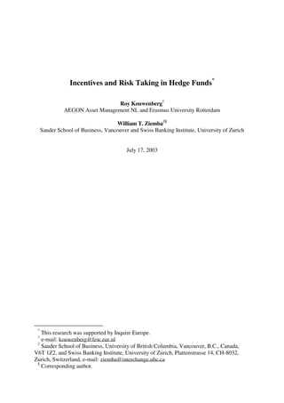
35. 34
Figure 1 Implicit level of loss aversion as a function of incentive fee
with fixed fee of =1%, lines for different levels of the manager'
s stake in the fund ( )
Incentive fee % ( )
Implicit
level
of
loss
aversion
(Â)
Figure 2 Optimal weight of stocks as a function of fund value
manager'
s stake in the fund =20%, lines for different levels of the incentive fee ( )
Fund value Y(t ) at time t = 0.5
Optimal
weight
of
stocks
= 30%
= 25%
= 20%
= 15%
= 0%

36. 35
Figure 3 Optimal weight of stocks as a function of fund value
incentive fee of =20%, lines for different levels of the manager'
s stake in the fund ( )
Fund value Y (t ) at time t = 0.5
Optimal
weight
of
stocks
= 100%
= 30%
= 20%
= 15%
= 10%
Figure 4 Initial weight of stocks as a function of the incentive fee
lines for different levels of the manager'
s stake in the fund ( )
0%
100%
200%
300%
Incentive fee ( )
Initial
weight
of
stocks
= 100%
= 30%
= 20%
= 10%

37. 36
Figure 5 Option value of 20% incentive fee,
as a function of the manager's stake in the fund ( )
0.00
0.05
0.10
0.15
0.20
Manager'
s stake in the fund ( )
Value
of
20
%
incentive
fee
(fund
value
=
1)
Figure 6 Optimal volatility of fund returns with incentive fee of 20%,
as a function of the manager stake in the fund ( )
0%
100%
200%
300%
400%
Manager'
s stake in the fund ( )
Volatility
of
hedge
fund
returns

38. 37
1
All of the following results are also valid for the case where the private portfolio’s return
R(0) is stochastic.
2
In this case we do not report additional results for a regression with incentive fee dummies
and management fee dummies as there are only a few funds with zero incentive fees, leading
to a lack of statistical power.