1. Lecture 1
Introduction to water and
wastewater treatment processes
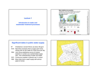
Significant dates in public water supply
97 Inhabitants in ancient Rome use about 38 gpcd
1619 New River Company first to supply each home
directly with its own water for a few hours per day
1854 John Snow establishes source of cholera
epidemic in London as a contaminated supply
well – first understanding of water and health
1873 Continuous supplies in general use in London
1900 Most cities have a water supply with service
pipes to homes
Source:
Environment
Canada,
2004.
Water
availability
versus
population.
http://www.ec.gc.ca/water/images/info/facts/e-Water_availability.jpg.
Accessed
December
10,
2004.
Source: Frerichs, Ralph R., 2005. John Snow. Department of Edipdemiology, School of Public Health, University
of California, Los Angeles, California. Updated January 1, 2005. Accessed January 4, 2005. http://www.ph.ucla.
edu/epi/snow.html. The map is reproduced from: Snow, John, 1855. On the Mode of Communication of Cholera.
John Churchill, London.
2. 0
100
200
300
400
500
600
700
(
)
)
0
20
40
60
80
100
120
140
160
180
)
U.S. total water use over time
Asia
excluding
Middle
East
Central
America
&
Caribbean
Europe
Middle
East
&
North
Africa
North
America
Oceania
South
America
Sub-Saharan
Africa
Developed
Countries
Developing
Countries
High
Income
Countries
Middle
Income
Countries
Low
Income
Countries
United
States
Domestic
water
use
(l/cap/day
Domestic
water
use
(gal/cap/day
Source for both images: Frerichs, Ralph R., 2005. John Snow. Department of Edipdemiology, School of Public Health, University of
California, Los Angeles, California. Updated January 1, 2005. Accessed January 4, 2005. http://www.ph.ucla.edu/epi/snow.html.
The map is reproduced from: Snow, John, 1855. On the Mode of Communication of Cholera. John Churchill, London.
Based on data from: World Resources Institute, 2004. EarthTrends, The Environmental
Information Portal, Water Resources and Freshwater Ecosystems, Searchable Database,
http://earthtrends.wri.org/searchable_db/index.cfm?theme=2. Accessed December 10,
2004.
Source: USGS, 2004. Water Science for Schools: Trends in water use. U.S. Geological Survey,
Washington, D.C. May 06, 2004. http://ga.water.usgs.gov/edu/totrendbar.html, accessed November 23,
2004. See also: Hutson, Susan S., Nancy L. Barber, Joan F. Kenny, Kristin S. Linsey, Deborah S. Lumia,
and Molly A. Maupin, 2004. Estimated Use of Water in the United States in 2000. Circular 1268. U.S.
Geological Survey, Reston, Virginia. May 2004. http://water.usgs.gov/pubs/circ/2004/circ1268/index.
html, accessed November 23, 2004.
3. Per
capita
use
(l/d/cap)
AL
AK
AZ
AR
CA
CO
CT
DE
FL
GA
HI
ID
IL
IN
IA
KS
KY
LA
ME
MD
MA
MI
MN
MS
MO
MT
NE
NV
NH
NJ
NM
NY
NC
ND
OH
OK
OR
PA
PR
RI
SC
SD
TN
TX
UT
VT
VI
VA
WA
WV
WI
WY
US
total
Average
350
US
VI
Domestic water use by state
1600
NEVADA
UTAH
MAINE
IDAHO
Per
capita
use
(gpd/cap)
1400
300
1200
250
1000
200
800
150
600
100
400
50
200
0 0
0
200
400
600
800
)
0
50
100
150
200
250
300
350
400
)
1000
1200
1400
1600
1800
2000
Baltimore,
MD
Berkeley,
CA
Boston,
MA
Grand
Rapids,
MI
Greenville
County,
SC
Hagerstown,
MD
Jefferson
County,
AL
Jefferson
County,
KS
Lancaster
County,
NE
Las
Vegas,
NV
Little
Rock,
AR
Los
Angeles,
CA
LA
County,
CA
Greater
Peoria,
IL
Memphis,
TN
Orlando,
FL
Rapid
City,
SD
Santa
Monica,
CA
Wyoming,
MI
US
average
Water
Consumption
(l/d/cap
Water
Consumption
(gpd/cap
Source: USGS, 2004. Water Science for Schools: Trends in water use. U.S. Geological Survey, Washington, D.C. May 06, 2004. http://ga.water.usgs.gov/edu/
totrendbar.html, accessed November 23, 2004. See also: Hutson, Susan S., Nancy L. Barber, Joan F. Kenny, Kristin S. Linsey, Deborah S. Lumia, and Molly A.
Maupin, 2004. Estimated Use of Water in the United States in 2000. Circular 1268. U.S. Geological Survey, Reston, Virginia. May 2004. http://water.usgs.gov/
pubs/circ/2004/circ1268/index.html, accessed November 23, 2004.
Source: USGS, 2004. Source and use of freshwater in the United States, 2000. http://ga.water.usgs.gov/edu/summary95.html.
Last Modified: May 06, 2004. Accessed November 23, 2004.
See also: Hutson, Susan S., Nancy L. Barber, Joan F. Kenny, Kristin S. Linsey, Deborah S. Lumia, and Molly A. Maupin, 2004.
Based on data from Hutson, Susan S., Nancy L. Barber, Joan F. Kenny, Kristin S. Linsey, Deborah S.
Lumia, and Molly A. Maupin, 2004. Estimated Use of Water in the United States in 2000. Circular
1268. U.S. Geological Survey, Reston, Virginia. May 2004. http://water.usgs.gov/pubs/circ/2004/
circ1268/index.html, accessed November 23, 2004.
Source of data: ASCE, 1979. Design and Construction of Sanitary and Storm Sewers. American Society
of Civil Engineers, New York, New York. Table 1, pp. 21-23.
4. (
)
8
4 8 4
0
2 2
6 6
(
)
8
8 4
4
0
o
o
12 12
12
A.M
400
200
600
800
1000
1200
1600
1400
1800
2000
2200
10 10
12
12 12
A.M
1600
1400
1200
1000
800
600
400
200
& Minimum Day
Water
Use
gpd
per
dwelling
unit
P.M
Time of Day
Daily Water Use Patterns,
Maximum Day & Winter Day
Typical Maximum Day
Typical Winter Day
Water
Use
gpd
per
dwelling
unit
P.M
Time of Day
Daily Water Use Patterns in
R-6 Area: Maximum Day
90 F Day without Rain
90 F Day with Rain
Figure by MIT OCW. Figure by MIT OCW.
Adapted from: Viessman, W., Jr., and M. J. Hammer. Water Supply and Pollution Control. 7th ed. Upper Saddle River, NJ: Pearson
Education, Inc., 2005.
0
i
(
l
it)
li
1890 1895 1900 1905 1910 1915 1920
70
80
90
100
120
130
10
30
50
70
90
Gallons
per
capita
Percentage
of
services
metered
Consumption & use of meters, Boston metropolitan district.
100
200
300
400
500
600
700
800
Leakage Domestic Spr nkling Total
Water
usage
gal
ons
per
day
per
dwel
ng
un
Metered
Flat-rate
110
Figure by MIT OCW.
Adapted from: Turneaure, F. E., H. L. Russell, and M. S. Nichols. Public Water
Supplies: Requirements, Resources, and the Construction of Works.
New York, NY: John Wiley & Sons, 1940.
Data from: Linaweaver, F. P., Jr., J. C. Geyer, and J. B. Wolff, 1967. A Study of Residential
Water Use, A Report Prepared for the Technical Studies Program of the Federal Housing
Administration, Department of Housing and Urban Development. Department of
Environmental Engineering Science, The Johns Hopkins University, Baltimore, Maryland.
5. 0
1
(
(
)
0
0
1
)
( )
3
2
1
(
)
(n)
20
40
60
80
100
120
32 53 94 125 156 187 218 248 280 342
1000
1200
1400
1600
1800
31 52 93 124 155 186 217 248 279 310 341 372 403
32 53 94 125 156 187 218 248 280 342
Daily min-max temperature, precipitation & water use in new york city for 1982.
Precipitation
311
Time day of year)
Min
&
Max
temperature
oF
311
Time (day of year
Time day of year
Total
water
use
mgd
0
0
0
0
( )
( )
(
)
(
)
20 40 60 80 100
-200
200
200
400
600
20 40 60 80 100
-200
-400
400
600
Deviations from annual average water use versus average daily temperature for 1982 & 1983
1983
1982
Avg Temperature oF
Avg Temperature oF
Diff
from
year
avg
water
use
mgd
Diff
from
year
avg
water
use
mgd
Figure by MIT OCW. Figure by MIT OCW.
Adapted from: Protopapas, A., S. Katchamart, and A. Platonova. "Weather effects on daily water use in New York City."
Journal of Hydrologic Engineering, ASCE 5, no. 3 (July 2000): 332-338.
1940
0
( )
?
0
(
/
)
i
12 12
10 10
2 2
4 4
6 6
8 8
0
20
40
80
80
80
60
60
60
100
120
120
160
160
160
100
100
120
140
140
140
180
40
40
180
180
200
ROCKFORD, III
Maximum Day
Maximum Day
Maximum Day
NOON
A.M
Hourly rates of consumption.
10
20
30
40
50
60
70
80
Precipitation
10
20
30
40
50
60
YEAR
Thousands
Daily water use -
1982 1983 1984 1985 1986 1987 1988 1989 1990 1991
MONTHLY AVERAGE TEMPERATURE & PRECIPITATION
Temperature oF
1982 1983 1984 1985 1986 1987 1988 1989 1990
Water
use
mga
month
Monthly average temperature, Precipitation, & water use in new York c ty for 1982 to 1991
MONTHLY WATER USE
Average
Temperature
&
Precipitation
Average Day
Maximum = 181% of Av.
Max. Hr.=188 x 181 = 340% Av.
Average per cap = 67.5 Gal.
MADISON, WIS.
Average Day
Maximum = 196% of Av.
Max.Hr.=175 x 196 = 343% Av.
Average per cap = 117 Gal.
MILWAUKEE, WIS.
Average Day
Maximum = 171% of Av.
Max.Hr.= 185 x 171 = 317% Av.
Average per cap = 138 Gal.
PERCENTAGES
P.M
Figure by MIT OCW. Figure by MIT OCW.
Adapted from: Protopapas, A., S. Katchamart, and A. Platonova. Adapted from: Turneaure, F. E., H. L. Russell, and M. S. Nichols.
"Weather effects on daily water use in New York City." Public Water Supplies: Requirements, Resources, and the
Journal of Hydrologic Engineering, ASCE 5, no. 3 (July 2000): 332-338.
Construction of Works. New York, NY: John Wiley & Sons, 1940.
6. 0
/d/
)
0
50
)
0%
10%
20%
30%
40%
50%
60%
70%
80%
90%
1950 1965 1970 1985 1990 2000
Per capita use of municipal water in United States
100
200
300
400
500
600
700
800
900
1000
1900 1910 1920 1930 1940 1950 1960 1970 1980 1990 2000
Per
capita
use
(l
cap
100
150
200
Per
capita
use
(gal/d/cap
Percent U.S. population served by municipal water supply
100%
1955 1960 1975 1980 1995
0
100
200
300
400
500
600
700
800
900
/d/cap)
0
50
100
150
200
/cap)
Surface-water drinking water plant
Surface-water
supply
Coagulant addition
and rapid mix
Flocculation Settling tank Filtration
Chlorine and
fluoride
Activated carbon
1000
Baltimore,
MD
Berkeley,
CA
Boston,
MA
Grand
Rapids,
MI
Greenville
County,
SC
Hagerstown,
MD
Jefferson
County,
AL
Jefferson
County,
KS
Lancaster
County,
NE
Las
Vegas,
NV
Little
Rock,
AR
Los
Angeles,
CA
LA
County,
CA
Greater
Peoria,
IL
Memphis,
TN
Orlando,
FL
Rapid
City,
SD
Santa
Monica,
CA
Wyoming,
MI
Wastewater
Generation
(l
Wastewater
Generation
(gpd
Based on U.S. Geological Survey. Estimated Use of Water in United States, Circulars 115, 398, 456, 556, 676, 765,
1001, 1004, 1081, 1200, 1268. Data for 1900 and 1924 from: Linaweaver, F. P., Jr., J. C. Geyer, and J. B. Wolff,
1967. A Study of Residential Water Use, A Report Prepared for the Technical Studies Program of the Federal Housing
Administration, Department of Housing and Urban Development. Department of Environmental Engineering
Science, The Johns Hopkins University, Baltimore, Maryland.
Based on U.S. Geological Survey. Estimated Use of Water in United States, Circulars 115, 398,
456, 556, 676, 765, 1001, 1004, 1081, 1200, 1268.
Source of data: ASCE, 1979. Design and Construction of Sanitary and Storm Sewers. American
Society of Civil Engineers, New York, New York. Table 1, pp. 21-23.
7. Intake Structure
Chemical Addition / Disinfection
Alum: Promote flocculation
Chattahoochee Water Treatment Plant –
River Flow
Sodium Hypochlorite: Disinfection
Courtesy of Joe Lin. Used with permission. Courtesy of Joe Lin. Used with permission.
Chemical mixing Flocculation / Sedimentation
Flocculation
Sedimentation
Courtesy of Joe Lin. Used with permission. Courtesy of Joe Lin. Used with permission.
8. Flocculation tank Sedimentation tank (clarifier)
Sludge scraper
Courtesy of Joe Lin. Used with permission. Courtesy of Joe Lin. Used with permission.
Filtration
Sedimentation tank collection troughs
Flow from sedimentation tanks
Courtesy of Joe Lin. Used with permission. Courtesy of Joe Lin. Used with permission.
9. Post-Treatment Chemical Addition
Fluoride: To prevent tooth decay
Lime: To raise the pH
Phosphoric acid: To prevent corrosion of piping in the distribution system
Sodium hypochlorite: To maintain disinfection residual in distribution system
Ground-water drinking water treatment plants
Disinfection and fluoridation
Iron and manganese removal
Chlorine Fluoride
Chlorine Fluoride
Chlorine or
permanganate
Aerator Filter
Contact
tank
Ground-water drinking water treatment plants
Softening
Aerator Flocculation
Mixer
Lime
Soda ash
Chlorine Fluoride
Filter
Settling tank Recarbonation
CO2
West Bridgewater, MA
water distribution
system
Image removed due to copyright reasons.
10. 0
200
400
600
800
1000
1200
1400
1600
1800
2000
)
0
50
100
150
200
250
300
350
400
)
l/
i (l/d/
Wastewater generated vs water used
Baltimore,
MD
Berkeley,
CA
Boston,
MA
Grand
Rapids,
MI
Greenville
County,
SC
Hagerstown,
MD
Jefferson
County,
AL
Jefferson
County,
KS
Lancaster
County,
NE
Las
Vegas,
NV
Little
Rock,
AR
Los
Angeles,
CA
LA
County,
CA
Greater
Peoria,
IL
Memphis,
TN
Orlando,
FL
Rapid
City,
SD
Santa
Monica,
CA
Wyoming,
MI
Rate
(l/d/cap
Rate
(gpd/cap
Water Consumption ( d/cap)
Wastewater Generat on cap)
4 8 8
4
0
(
)
( ) ( )
12
200
400
600
AM PM
NOON
occurred.
Time of Day June 23,1961
Water
use
and
wastewater
flow
gpd
per
service
Comparison of water use solid line & wastewater flow dashed lines on days when little sprinkling
WATER
WASTEWATER
Figure by MIT OCW.
Adapted from: Viessman, W., Jr., and M. J. Hammer. Water Supply
and Pollution Control. 7th ed. Upper Saddle River, NJ: Pearson
Education, Inc., 2005.
Toil
fl
Bathi
5%
Typical Domestic Water Use
et
ushing
40%
ng
30%
Laundry
15%
Kitchen
10%
Other
1
2
4
5
C C D C A B C D D
C D D
E D B
0
2400
2200
2000
1800
1600
1400
1200
1000
0800
0600
0400
0200
0000
1.0
2.0
3.0
4.0
5.0
Peak Demand
Duration-min Gal
15
60
10
20
26
64
Demand rates calculated over 4-min intervals were used.
Total Daily Use: 245 Gal. A - Home Laundry
B - Dishwasher
C - Foodwaste Disposer
D - Shower
E- Bath
Water
Demand
-
gpm
Water Use
TYPICAL DAILY HYDROGRAPH FROM TEST HOME II
Figure by MIT OCW.
Adapted from: Anderson, J. S., and K. S. Watson. "Patterns of household
usage." Journal American Water Works Association 59, no. 10 (October
1967): 1228-1237.
Source of data: ASCE, 1979. Design and Construction of Sanitary and
Storm Sewers. American Society of Civil Engineers, New York, New
York. Table 1, pp. 21-23.
Data from: Droste, R. L., 1997. Theory and Practice of Water and Wastewater
Treatment. John Wiley & Sons, Hoboken, New Jersey.
11. Pollutants in domestic wastewater
High strength Medium strength Low strength
TSS, Total suspended solids (mg/L) 120 210 400
BOD, 5-day biochemical oxygen demand (mg/L) 110 190 350
Ammonia nitrogen (mg/L as N) 12 25 45
Organic nitrogen (mg/L as N) 8 15 25
Total phosphorus (mg/L) 4 7 12
Oil and grease (mg/L) 50 90 100
Total coliform bacteria (number/100 ml) 106 – 108 107 – 109 107 - 1010
Fecal coliform bacteria (number/100 ml) 103 – 105 104 – 106 105 - 108
Cryptosporidium oocysts (number/100 ml) 0.1 - 1 0.1 - 10 0.1 – 100
Giardia lamblia cysts (number/100 ml) 0.1 – 10 0.1 - 100 0.1 - 1000
0 2 4 6 8
0 0
/m
3
/h
3
/s
10 14 16 18 20 22 24
50
100
150
200
250
300
0.05
0.1
0.2
0.15
Midnight Midnight
Noon
BOD
concentration,
g
&
BOD
mass
loading,
kg
Flowrate,
m
Flowrate
BOD Concentration
BOD Mass Loading
Time of Day
Typical hourly variations in flow & strength of domestic wastewater.
Figure by MIT OCW.
Adapted from: G. Tchobanoglous, F. L. Burton, and H. D. Stensel.
Wastewater Engineering: Treatment and Reuse. 4th ed. Metcalf &
Eddy Inc., New York, NY: McGraw-Hill, 2003.
Sludge
thickening
Sludge
digestion
Bar
Screen
Grit
Chamber
Primary
settling
Activated sludge
biological treatment
Final
settling
Contact
basin
Chlorination
Activated sludge recycle
Bar
Screen
Grit
Chamber
Primary
settling
Activated sludge
biological treatment
Final
settling
Contact
basin
Chlorination
Activated sludge recycle
Typical wastewater treatment plant Typical wastewater treatment plant
Preliminary
treatment
Primary
treatment
Secondary
treatment
Disinfection
Can also have tertiary treatment to remove nutrients and other pollutants
Based on Metcalf & Eddy Inc., G. Tchobanoglous, F. L. Burton, and H. D. Stensel, editors,
2003. Wastewater Engineering: Treatment and Reuse, Fourth Edition. McGraw-Hill, New
York. Table 3-15, pg. 186.
12. Lynn, MA wastewater treatment plant
chambers
Bar
screens
Grit
Bar screens
Bar screens Traveling screen
16. LECTURE 1
INTRODUCTION TO WATER QUALITY AND TREATMENT, OVERVIEW OF
WASTEWATER AND TREATMENT PROCESSES
Water supply
Slide 2 - Volumetric water use in the United States
US is in a relatively water-rich part of the world, although there are obviously
local exceptions
Slide 3 - Per capita use for domestic water supply
US is one of largest water users – using 600 l/cap/day = 160 gal/cap/day
Slide 4 – Significant events in history of water supply
Most of the world still does not have centralized water supply with connections to
individual households
According to the World Health Organization roughly 1 billion of the world’s
6 billion people do not have access to an improved water supply.
JMC, 2000. Global Water Supply and Sanitation Assessment 2000 Report. WHO and
UNICEF Joint Monitoring Programme for Water Supply and Sanitation, World Health
Organization and United Nations Children’s Fund,
http://www.who.int/docstore/water_sanitation_health/Globassessment/Global2.1.htm.
Accessed January 4, 2005.
Access to water-supply services is defined as the availability of at least 20 litres
per person per day from an "improved" source within 1 kilometre of the user's
dwelling. An “improved” source is one that is likely to provide "safe" water,
such as a household connection, a borehole, etc.
JMC, 2004. The Joint Monitoring Programme : definitions. WHO and UNICEF Joint
Monitoring Programme for Water Supply and Sanitation, World Health Organization and United
Nations Children’s Fund, http://www.wssinfo.org/en/122_definitions.html. Accessed January 4,
2005.
An improved water supply is defined as:
• Household connection
• Public standpipe
• Borehole
• Protected dug well
• Protected spring
• Rainwater collection
JMC, 2000. Global Water Supply and Sanitation Assessment 2000 Report. WHO and
UNICEF Joint Monitoring Programme for Water Supply and Sanitation, World Health
Organization and United Nations Children’s Fund,
http://www.who.int/docstore/water_sanitation_health/Globassessment/Global2.1.htm.
Accessed January 4, 2005.
Only 48% of the world’s population is connected at the household level.
JMC, 2004. Water supply data at global level. WHO and UNICEF Joint Monitoring
Programme for Water Supply and Sanitation, World Health Organization and United Nations
Children’s Fund, http://www.wssinfo.org/en/22_wat_global.html. Accessed January 4, 2005.
Slides 5, 6, & 7 – Dr. John Snow’s analysis of cholera deaths in London in 1854.
First study to show connection between contaminated water and impaired public
health
1
17. Slides 8 & 9 - Patterns of water use
Total US water use increased steadily until 1980s, but largely due to cooling
water use for electric power
Rate of increase exceeded rate of population increase
Since 1980s water use has leveled off despite population increase
Slide 9 – increase of public water supply has been slower but unabated
Slide 10 - Sources of drinking water in US
Ratio of 3:1 surface water:ground water for overall use but heavier reliance on
ground water for public water supply
Slides 11 & 12 – Large geographical variation within US
Greater domestic water use in arid areas – mostly for landscaping
Note low use in Virgin Islands – established practice of conservation: “In this land
of fun and sun, we don’t flush for number 1”
Maine - ???
Slide 12 – large variation also holds true for cities – Las Vegas has high water
use for outdoor watering, not hotels as one might expect (Carmen Roberts,
Vegas heading for ‘dry future’. BBC News, July 29, 2005.
http://news.bbc.co.uk/1/hi/sci/tech/4719473.stm)
Slides 13, 14, & 15 – Johns Hopkins study of water use
Classic study completed in 1960s by Johns Hopkins University
Conducted 1961-66
Continuous monitoring of water use by 41 homogenous residential areas
with 44 to 410 dwelling units and several apartment areas
Covered: 16 different water supply utilities, 11 metropolitan areas; 6
different climatic regions
Slide 13
Winter graph shows household usage – morning and early evening peaks
Summer graph shows potentially profound effect of sprinkling
Slide 14 shows summer usage with and without rainfall
Factors affecting water use:
Income – rich people use more water
Climate – more water is used in dry climates (for watering lawns)
Season – less water is used in winter than summer
Metering – metered customers used less water for watering lawns than
those on flat rates
Slide 15 shows effect of metering on water use: little effect on household use but
major effect on sprinkling
Slide 16 – Relation of water use to metering is not a new story – this graph is from
textbook dated 1940
After the change in economic systems in eastern Europe, there was concern
about how to bring wastewater treatment systems up to western standards.
Many were highly overloaded before the change, but once the authorities
started to charge for water, usage went down, wastewater went down, and
overloaded plants were no longer overloaded
Slides 17, 18, & 19 – Study of effect of weather on New York City supply
Slide 17 – use during 1982 shows fairly constant use until it gets hot – above
72ºF water use increases linearly with temperature
Slide 18 – shows same pattern in 1983
2
18. Slide 19 – pattern is absent in 1985 – why? Mandatory water conservation
measures imposed by city
Slide 20 – pattern of daily water use has not changed appreciably over the years – curve
for 1940 shows morning and afternoon peaks in usage
Slide 21 – shows that total usage increased, at least until around 1980
Slide 22 – despite prevalence of public water supply systems, about 20 percent of the
US population is self supplied – usually by a ground-water well. This fraction has
not changed appreciably for many decades.
Slides 24-33 - Walk-through of typical water treatment process
Slides 34&35 – Ground-water systems
Slide 34a – often minimal treatment is required
Slide 34b – Ground waters often high in iron and manganese (particularly in New
England)
Removed by oxidizing to insoluble iron oxide (rust) or manganese oxide,
which precipitate and can be removed by filtration
If not removed in treatment plant, iron and manganese precipitate in
distribution system and cause staining of laundry, fixtures, etc.
Slide 35 – Deep, old ground waters are often highly mineralized and “hard” (high
concentrations of Ca and Mg)
Water is softened by adding lime (Ca(OH)2) and soda ash (Na2CO3)
Recarbonation removes excess lime and prevents scaling of equipment
and pipes
Slide 36 – Water distribution systems brings treated water to homes and businesses –
not covered in this course
Wastewater
Slides 37 and 38 – water supply begets wastewater generation, usually with a pretty
close correlation
Slide 37 – Exceptions are:
water supply > wastewater when sprinkling use is great (e.g., Las Vegas, Los
Angeles) and/or exfiltration from sewers is high
water supply < wastewater when infiltration into sewers is high (perhaps
Greenville County?)
Slide 38 – Johns Hopkins study confirms this on day with little sprinkling
Slide 39 – Most water used in the household becomes wastewater via various routes
Consumption (drinking, cooking) is pretty negligible
Toilets use the most, hence low-flow toilets are a good water conservation
measure
Slide 40 – Daily flow curves are averages over many households – the flow from
individual household is very episodic
Under some circumstances, flow from individual homes can be coordinated:
wastewater treatment plant workers in New York City claim to be able to tell
the popularity of TV shows by the wastewater surge seen during commercials
Slide 41 – Wastewater quality
BOD, TSS – for short-term effect on receiving water
3
19. N, P – for long-term effect (eutrophication) on receiving water
Oil and grease – for short-term effect
Pathogens – for effects on human health
Slide 42 – Variation in flow also causes variation in strength of wastewater – Why?
At low flow, solids settle, reducing BOD concentration
At high flow, solids get scoured from pipes, increasing BOD concentration
Slides 43-49 – Walk-through of typical wastewater treatment process
Slide 50 – Virtual tours of WWTPs: (really should be “scratch and sniff”)
Englewood, Colorado – http://www.englewoodgov.org/wwtp/
Lynn, Massachusetts – http://members.aol.com/erikschiff/prelim.htm
Lexington, Kentucky – http://www.lfucg.com/sewers/TBTour.asp
4