1. 1
An Examination of the Water Budget in the
Middle Potomac-Anacostia-Occoquan Watershed
Hydrology and Water Resources
Watershed Report
Mike Stoever
ABSTRACT
The Potomac River basin provides the surface and groundwater resources to the
Washington, D.C. metro region and is home to approximately 6.1 million people, the majority of
whom live within the Middle Potomac-Anacostia-Occoquan watershed. Therefore, in order to
ensure that their water supply needs are and will continue to be met, an accurate characterization
of the water budget for the latter watershed is essential. This study reviews the existing literature
on the topic and utilizes data provided by U.S. Geological Survey (USGS) monitoring stations in
the District of Columbia, Maryland, and Virginia in order to begin this process. An intensity-
duration-frequency curve and flow duration curve were created to help estimate future annual
rainfall and potential locations of heavy runoff and minimal groundwater recharge, respectively,
along with a plotting of the relationship between evapotranspiration, precipitation, and discharge
in the watershed. When taking into account the geologic and climatic conditions of the
watershed, these graphs show that low flows and precipitation levels in the summer months may
result in diminished water availability during drought conditions. Further, it is hoped that these
results will shine a light on the need to ensure that annual water budget estimates do not obscure
water supply problems during these months, as has often proven to be the case relative to
seasonal water budget estimates.
INTRODUCTION
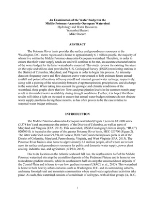
The Middle Potomac-Anacostia-Occoquan watershed (Figure 1) covers 833,808 acres
(3,374 km2
) and encompasses the entirety of the District of Columbia, as well as parts of
Maryland and Virginia (EPA, 2015). This watershed, USGS Cataloging Unit (or simply, “HUC”)
02070010, is located at the center of the greater Potomac River basin, HUC 020700 (Figure 2).
The latter watershed covers 9,394,427 acres (38,017 km2
) and encompasses parts or all of the
District of Columbia, Maryland, Pennsylvania, Virginia, and West Virginia (EPA, 2015). The
Potomac River basin is also home to approximately 6.1 million people, all of whom are reliant
upon its surface and groundwater resources for public and domestic water supply, power plant
cooling, industrial use, and agriculture (ICPRB, 2015).
Due to its location on the Atlantic seaboard fall line, the northwestern half of the Middle
Potomac watershed sits atop the crystalline deposits of the Piedmont Plateau and is home to low
to moderate gradient streams, while its southeastern half sits atop the unconsolidated deposits of
the Coastal Plain and is home to very low gradient streams (USACE et al., 2013). This watershed
is home to both heavily urbanized areas such as Washington, D.C. and its surrounding suburbs,
and many forested rural and mountain communities where small-scale agricultural activities take
place. As such, this watershed consists of a multitude of soil types, with all four groups (A, B, C,

2. 2
Figure 1: Location of the Middle Potomac-Anacostia-Occoquan watershed.
SOURCE: EPA, 2016.
Figure 2: Location of the Potomac River basin.
SOURCE: Tiruneh, 2007.
D) and three dual classes (A/D, B/D, C/D) of soils represented (Tiruneh, 2007; USDA, 2016). As
one might expect, the soils found in or near urban areas tend to be more representative of Group
C or D soils, while those in rural areas tend to be more Group A or B soils (USDA, 2016). The
geologic setting also plays a role here, with the soils overlying the Piedmont Plateau displaying
more infiltrative ability compared to the poorly drained, fine textured soils (such as clays)
overlying the Coastal Plain (USACE et al., 2013).

3. 3
Land use in the Middle Potomac watershed is representative of that in the Potomac River
basin as a whole. As depicted in Figure 3, the latter basin is predominantly forested, with smaller
areas of agriculture and urban development found within (USGS, 1998). Correspondingly, the
Middle Potomac watershed’s western side is mostly forested, its central area heavily agricultural,
and its eastern side heavily urbanized (USACE et al., 2013).
Befitting a basin whose drainage to the Chesapeake Bay is second only to the
Susquehanna River basin, the namesake Potomac River flows 283 miles in a generally
southeastern direction with an average discharge at its mouth of 14,300 cfs (USACE et al.,
2013). Tidally influenced for its last 113 miles, flow in the majority of streams in the basin is
sustained by groundwater discharge during dry periods, resulting in comparable water quality
between stream water and groundwater (USGS, 1998; USACE et al., 2013). However, USGS
(1998) is careful to note: “When flows are elevated during storms, streams of the basin typically
become concentrated in chemicals that are washed from the land, although streams in some areas
may become diluted.” Thus, stormwater runoff is of high concern in this watershed with regards
to its potentially negative impacts on water quality.
The Middle Potomac watershed (and Potomac River basin overall) receives a fairly even
distribution of precipitation throughout the year, with an area-weighted mean of 42 in/yr over the
past 30 years (USGS, 2016). Due to a location in the Mid-Atlantic seaboard, its climate is
temperate with well-defined seasonal change and corresponding increases or decreases in
precipitation and flow. For example, USACE et al. (2013) found that summer lows in stream
flow can primarily be attributed to watershed losses due to evapotranspiration (ET) that occurred
between the months of March and September. Further, the preponderance of forests in the region
(which cover 63 percent of the basin west of the fall line) drives this evapotranspirative process,
which has an area-weighted mean actual ET of 22 in/yr (USACE et al., 2013; USGS, 2016).
Flow levels are lowest in the warmer summer months when precipitation is less common and
snowmelt has been depleted. However, high flows are seen throughout the region year-round.
This is due to their being driven by storm events that are stochastic in nature. Average annual
precipitation and evapotranspiration for the Potomac River basin is shown in Figure 4.
Figure 3: Land use types in the Potomac River basin.
SOURCE: Tiruneh, 2007.

4. 4
a b
Figure 4: Average annual precipitation (a) and evapotranspiration (b) in inches in the Potomac River
basin.
SOURCE: Tiruneh, 2007.
METHODS
Due to the sheer volume of monitoring stations within the Potomac River basin, I
restricted my analyses to the Middle Potomac-Anacostia-Occoquan watershed (HUC 02070010).
Area-weighted mean daily precipitation and monthly actual evapotranspiration data were
obtained from the USGS National Water Census Data Portal for 1980-2014 and 2000-2014,
respectively. The smaller data set for evapotranspiration was due to data limitations (i.e., no data
was available for years prior to 2000). Mean daily and monthly discharge values for Water Year
2015 (10/1/14 – 9/30/15), the most recent Water Year where data were fully available, were
obtained from the USGS National Water Information System for three USGS monitoring stations
randomly selected from within the HUC. USGS 01648000 represented the District of Columbia
and was located at Rock Creek at Sherrill Drive; USGS 01650800 represented Maryland and was
located at Sligo Creek near Takoma Park, MD; and USGS 01656000 represented Virginia and
was located at Cedar Run near Catlett, VA. These values were then imported into Microsoft
Excel for further analysis, detailed below.
IDF Curve
Once imported into Microsoft Excel, the area-weighted mean precipitation values for
1980-2014 within this HUC were then summed up to represent annual totals and these values
were then converted from millimeters to inches. Next, the data were sorted according to their
ranking from largest to smallest and the Weibull method was used to obtain the return period (in
years) for the data. For example, the return period for the first ranking was 𝑇 =
!!!
!
=
!"!!
!
=
36.0, where T is the return period, y is the total number of events, and n is the rank of the event.
This information was then plotted with the return period values on the x-axis and the rainfall
amounts on the y-axis. The two axes were then set to a logarithmic scale giving the graph a log-

5. 5
log scale, and a trend line of best fit was fitted to the displayed data. The expected annual rainfall
for the return periods of 2, 20, and 100 years were then calculated.
Flow Duration Curve
Once imported into Microsoft Excel, the mean daily discharge values (in cfs) for each set
of data were ranked by magnitude. The exceedence probabilities for each entry were calculated
as 𝐸𝑃 = 100 ∗
!
!!!
where EP is the exceedence probability, n is the rank of the event and y is the
total number of events. In order to compare the three streams, the curves were plotted on the
same graph using q/A (on a log scale on the vertical axis), where q is the discharge value and A is
the drainage area. The drainage area for USGS 01648000 was 62.2 mi2
; the drainage area for
USGS 01650800 was 6.45 mi2
; and the drainage area for USGS 01656000 was 93.4 mi2
.
Annual actual evapotranspiration, precipitation, and discharge
Once imported into Microsoft Excel, the area-weighted mean actual evapotranspiration
(AET) values for 2000-2014 within this HUC were then summed to represent yearly (instead of
their original monthly) totals and these values were then converted from millimeters to inches.
These values were then plotted against the precipitation values for those years that were
calculated when creating the IDF curve. Additionally, the monthly AET values for the year 2014
were plotted in a separate graph against the monthly precipitation values for that year to show the
relationship between these two variables in a calendar year. The deviation from Water Year 2015
to calendar year 2014 was due to limited AET data availability for the former. The daily
precipitation values for that year were summed up to represent monthly values in the latter graph.
Finally, the monthly discharge values for Water Year 2015 from the three monitoring stations
were plotted together on a separate graph to show the relationship between discharges at the
different stations.
RESULTS
IDF Curve
As shown in Figure 5 below, once plotted the trend line of best fit (i.e., one with an r2
>
0.9) was found to be a logarithmic trend line with an r2
of 0.95416. Using the fitted trend line and
its equation 𝑦 = 7.7706 ln 𝑥 + 34.512, the expected annual rainfall for a return period of 2
years was calculated to be 39.9 in, 20 years 57.8 in, and 100 years 70.3 in (substituting 2, 20, and
100 in for x).

6. 6
Figure 5: Intensity-Duration-Frequency (IDF) curve using the Weibull method.
Flow Duration Curve
Once plotted, the data in Figure 6 (shown below) displayed distinctive steep upper curves
at all three sites. However, the Virginia site displayed a steeper lower curve when discharge was
equaled or exceeded 60 percent of the time or higher. This implies a difference in amount of
urbanization and infiltrative capacity amongst the three sites, particularly between Virginia and
the District of Columbia and Maryland sites.
y
=
7.7706ln(x)
+
34.512
R²
=
0.95416
1
10
100
1
10
100
Rainfall
(in)
Return
period
(years)

7. 7
Figure 6: Flow duration curve for three streams within HUC 02070010.
Annual actual evapotranspiration, precipitation, and discharge
When plotted (see Figure 7 below), AET displays little yearly variability from 2000-
2014, especially when compared to precipitation over that same period. Further, when values for
calendar year 2014 were plotted together on a separate graph (Figure 8), evapotranspiration
displays an expected parabolic shape. That is, it is higher in the warmer spring/summer months
than it is in the cooler fall/winter months. Precipitation over this period displays a slightly
unexpected shape, with diminished amounts in the warmer summer months overall yet a total in
August comparable to the wetter spring months. Additionally, when plotted together (Figure 9)
the monthly discharge rates amongst the three monitoring stations show noticeable deviation.
Monitoring station 01656000 (in VA) showed the greatest range, including the highest flow rate,
and monitoring station 01650800 (in MD) was significantly lower than the other two stations and
displayed the least similarity to the others.
0
1
10
100
0
20
40
60
80
100
Discharge
(cfs/mi^2)
Percent
of
time
that
indicated
discharge
was
equaled
or
exceeded
Station
01648000
(DC)
Station
01650800
(MD)
Station
01656000
(VA)

8. 8
Figure 7: AET vs. precipitation in HUC 02070010 for the years 2000-2014.
Figure 8: AET vs. precipitation in HUC 02070010 for the 2014 calendar year.
0
10
20
30
40
50
60
70
2000
2002
2004
2006
2008
2010
2012
2014
Inches
of
evapotranspiration
/
precipitation
Year
Annual
precipitation
Average
annual
precipitation
Annual
AET
0
1
2
3
4
5
6
7
Jan
Feb
Mar
Apr
May
Jun
Jul
Aug
Sep
Oct
Nov
Dec
Inches
of
evapotranspiration
/
precipitation
Month
Precipitation
Evapotranspiration

9. 9
Figure 9: Mean monthly discharge values in HUC 02070010 for Water Year 2015.
DISCUSSION AND CONCLUSION
The Middle Potomac watershed and the greater Potomac River basin are unique in that
they extend westward from a heavily urbanized area located directly over the Atlantic seaboard
fall line to a mostly forested, rural area. Thus, the watershed and its greater basin possess “very
distinct geologic, geomorphic, hydrological and landuse/landcover characteristics that vary
across the region” (Tiruneh, 2007). These characteristics, along with the climate of the Mid-
Atlantic region, play a great role in regulating the fluxes of the hydrologic cycle and water
budget of the region, which themselves are subject to varied flow inputs and levels, stormwater
runoff amounts, and the aforementioned diverse land uses.
As USACE et al. (2013) note, the deforestation and urbanization that occurs in
watersheds such as these increase stormwater runoff and can change “the magnitude, frequency,
duration, and possibly the timing of stream flows”. Further, the presence of a high level of
impervious surfaces in a watershed can result in flashier, more erosive streams (USACE et al.,
2013). These differences in land use and their resultant effects on the water budget and
hydrologic cycle of the watersheds are especially noticeable under analysis.
As seen in the flow duration curve depicted in Figure 6, the stations in DC and MD
display characteristics typical of flashy, urban watersheds. Curves for such watersheds often
have the steep upper and lower ends displayed by the data collected at these two stations,
indicating that their discharges are heavily determined by climate and precipitation (shown at the
upper end of the curves) and geology and topography (shown at the lower end of the curves).
That is, they are likely highly influenced by flashy, short duration storms and are located in areas
with an absence of significant groundwater or aquifer storage. This lack of significant subsurface
0
50
100
150
200
250
Oct
Nov
Dec
Jan
Feb
Mar
Apr
May
Jun
Jul
Aug
Sep
Discharge
(cfs)
Month
Station
01648000
(DC)
Station
01650800
(MD)
Station
01656000
(VA)

10. 10
storage results in higher flow variability, often due to the shortened residence time of the
contributing water source.
Comparatively, the station in VA looks to be in a more suburban or forested location, as
it displays a steep upper end (indicating heavy influence of climate and rainfall) but a flatter
lower curve, indicating that it benefits from a different geology and topography than its two
counterparts in this study. Thus, a relatively large percentage of its flow is likely coming from
storage in groundwater aquifers or frequent precipitation inputs. Knowing that this monitoring
station is located on the western side of the fall line, where the underlying substrate is that of the
Piedmont Plateau while the other two are located in the Coastal Plain, this may indeed be the
case. However, the lowered variability of flow that comes with heavy groundwater input is not
seen at this monitoring station when viewing its monthly discharges for Water Year 2015 (Figure
9). As this site is located in a suburban region where urbanization is occurring (it is indeed
implied in the name, after all) it is reasonable to see higher variability here relative to a truly
forested, rural area. Further, the suburban location of this site may actually help explain the
higher than expected variability shown in Figure 9. As it is receiving contributions from both
urban runoff and lag-induced groundwater flow, the potential is there for increased highs and
lows when its discharge values are plotted.
It must be said that the relatively low levels of discharge shown at the MD site may also
be attributed to the impaired nature of the water body being sampled. Sligo Creek, which is one
of 14 tributaries to the Anacostia River and thus to the Chesapeake Bay, has long suffered from
high levels of stormwater runoff and habitat destruction (MDE, 2012). It is listed as a 303(d)
impaired water under the Clean Water Act and has been the focus of an extensive, multi-year
restoration progress to reduce peak flow discharge and improve water quality, streambed and
bank stability, and in-stream habitat (MDE, 2012).
As shown in Figures 7 and 8, seasonality appears to play a factor in the interannual
variability surrounding these monitoring locations and the Middle Potomac watershed as a
whole. High, regular amounts of precipitation are seen in the fall, winter, and spring seasons,
while more stochastic precipitation amounts are observed in summer months. This can likely be
attributed to the intense, short duration thunderstorms that often occur in the region during these
months. Evapotranspiration responds accordingly, with a parabolic curve representing higher
rates during warmer months displayed for the calendar year 2014.
In terms of understanding these hydrologic fluxes, it is important to create IDF curves
such as the one shown in Figure 5 to assist in the prediction of expected annual rainfall. For
example, Figure 5 enables the prediction of the expected annual amount of this input in 2, 20,
and 100 years, such as was detailed in the results section of this study. Additionally, the stability
of the relationship between precipitation and evapotranspiration as shown in Figure 8 is
important to see. This is especially truthful when taking into account yearly discharge values
(Figure 9) when planning for future surface and groundwater withdrawals and uses, such as the
reliance of the urban areas within the Middle Potomac watershed and Potomac River basin on
waterways for their drinking water supplies.
The author of this study is careful to note that were some drawbacks to its methodology.
Primarily, time constraints and limited data availability from USGS for the Middle Potomac
watershed resulted in only three monitoring stations being analyzed. While helpful in getting an
overall understanding of the water budget for this watershed, sampling from a higher number of

11. 11
monitoring stations is recommended in order to get a more detailed, representative view of its
hydrologic fluxes and variability.
As the greater Washington, D.C. region continues to grow, the surface water and
groundwater resources of the Middle Potomac watershed and Potomac River basin will likely
encounter greater stresses. It is imperative that detailed studies take place to fully account for the
amount of groundwater recharge taking place, especially in upstream areas where many
homeowners rely on aquifers for their water supply. Increased pumping upstream without
sufficient recharge may lead to decreased surface water supplies downstream, a problem that
may be particularly acute during times of drought. As Tiruneh (2007) noted, “Increasing demand
for water associated with population growth and weather anomalies that result in drought may
strain the water resources of the [Potomac River] basin.” Further, coordination between groups
analyzing seasonal and annual water budgets is strongly recommended. Annual analysis of
recharge estimates, which include the high levels of recharge that occur during the fall and
winter months, often obscures potential problems related to water supply in the summer months,
an issue compounded by the poor ability of the region’s aquifers to store recharge (ICPRB,
2004). Comparatively, seasonal water budget analyses commonly predict lower water
availability during summer months than what is estimated by annual recharge (ICPRB, 2004).
REFERENCES
EPA (U.S. Environmental Protection Agency). 2015. MyWATERS Mapper. Available online at:
https://map24.epa.gov/mwm/mwm.html?fromUrl=05030101. Accessed November 12,
2016.
EPA. 2016. Surf Your Watershed: Middle Potomac-Anacostia-Occoquan Watershed –
02070010. Available online at: https://cfpub.epa.gov/surf/huc.cfm?huc_code=02070010.
Accessed November 14, 2016.
ICPRB (Interstate Commission on the Potomac River Basin). 2004. Annual and Seasonal Water
Budgets for the Monocacy/Catoctin Drainage Area. Available online at:
https://www.potomacriver.org/wp-content/uploads/2014/12/ICPRB04-4.pdf. Accessed
November 17, 2016.
ICPRB. 2015. The Potomac River Basin. Available online at: https://www.potomacriver.org/wp-
content/uploads/2014/11/Potomac-Basin-Fact-Sheet_Oct_2015.pdf. Accessed November
17, 2016.
MDE (Maryland Department of the Environment). 2012. Stream Restoration Reduces Peak
Storm Flow and Improves Aquatic Life in Sligo Creek. Available online at:
http://www.mde.state.md.us/programs/Water/319NonPointSource/Documents/Success%
20Stories/md_sligo-success-story_EPA-final.pdf. Accessed November 17, 2016.
Tiruneh, N. 2007. Basin-wide Annual Baseflow Analysis for the Fractured Bedrock Unit in the
Potomac River Basin. Available online at: http://www.potomacriver.org/wp-
content/uploads/2014/12/ICPRB07-6.pdf. Accessed November 14, 2016.
USACE (U.S. Army Corps of Engineers), TNC (The Nature Conservancy), and Interstate
Commission on the Potomac River Basin. 2013. Middle Potomac River Watershed
Assessment: Potomac River Sustainable Flow and Water Resources Analysis. Available
online at: http://www.potomacriver.org/wp-

12. 12
content/uploads/2015/01/MPRWA_FINAL_April_2013.pdf. Accessed November 14,
2016.
USDA (U.S. Department of Agriculture). 2016. NRCS Web Soil Survey. Available online at:
http://websoilsurvey.sc.egov.usda.gov/App/WebSoilSurvey.aspx. Accessed November
13, 2016.
USGS (U.S. Geological Survey). 1998. Water Quality in the Potomac River Basin, Maryland,
Pennsylvania, Virginia, West Virginia, and the District of Columbia, 1992-96: U.S.
Geological Survey Circular 1166. Available online at:
http://water.usgs.gov/pubs/circ1166. Accessed November 12, 2016.
USGS. 2016. National Water Census Data Portal: Available Water Budget Components.
Available online at: http://cida.usgs.gov/nwc/#!waterbudget/huc/02070010. Accessed
November 14, 2016.