PetroTeach Free Webinar on Seismic Reservoir Characterization
160425Seattle_AtmosSciSeminar_Chaplin
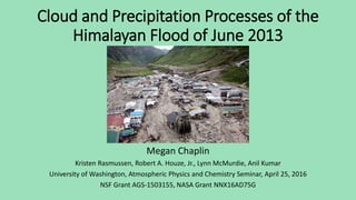
1. Cloud and Precipitation Processes of the
Himalayan Flood of June 2013
Megan Chaplin
Kristen Rasmussen, Robert A. Houze, Jr., Lynn McMurdie, Anil Kumar
University of Washington, Atmospheric Physics and Chemistry Seminar, April 25, 2016
NSF Grant AGS-1503155, NASA Grant NNX16AD75G
2. INDIA
Tibetan Plateau
Bay of
Bengal
Arabian
Sea
UTTARAKHAND
4TH CONSECUTIVE YEAR
OF FLOODING
•Continuous rainfall and snow at high elevations
•Flash flooding AND landslides
•5700 presumed dead
•4200 villages affected
•Flooding common and highly disruptive
•Broad stratiform precipitation RARE
MONSOON SEASON
UTTARAKHAND
Romatschke et al. 2010
PROBABILITY OF BROAD STRATIFORM
5. Objectives
• Non-convective
• Baroclinic wave in the westerlies
• Synoptic features + prior rain + orography
Methodology
• Reanalysis, satellite, radar observations, and model output
• Describe the synoptic, mesoscale, and orographic
characteristics
• Understand how characteristics led to massive flooding,
similar in strength to floods due to convection
Features of the flood producing storm
15. TRMM Precipitation Radar
•Spaceborne satellite radar
•3D maps of storm
structure
•INFORMATION ON:
•Intensity and
distribution of rain
•Rain type
•VERTICAL STRUCTURE
19. MODELING
Can model simulate:
• Type of precipitation
• Dynamics of storm system
Hypotheses to test:
• Non-convective/stratiform
• Orographically enhanced
• Baroclinically driven system
Goal:
• Better predictability
20. 15 N
20 N
25 N
30 N
35 N
10 N
5 N
60 E 70 E 80 E 90 E 100 E
Domain: 9, 3, 1 km Domain: 81 and 27 km
0 N
15 N
30 N
45 N
15 S
45 E 60 E 75 E 90 E 105 E
21. 500 hPa WRF Q-VECTORS
6/17 0600 UTC
RED SHADING: CONVERGENCE
BLUE SHADING: DIVERGENCE
MODELED SYNOPTIC FORCING
22. 6/17
0600
500 hPa 700 hPa
Vectors: horizontal wind vectors
Dark red shading: upward motion
Blue shading: subsidence
WRF VERTICAL VELOCITIES
MODELED MESOSCALE FORCING
23. COMPARISON OF MODEL AND RADAR
06/17 0700 UTC
WRF MIXING RATIOS
S Distance (km) N
0 100 200 300 400 500
0.0
2.0
4.0
6.0
8.0
10.0
12.0
14.0
16.0
18.0
20.0
Height(km)
Shading: rain water
Black : graupel
Green: snow
Blue: cloud ice
Grey: temperature
24. COMPARISON OF MODEL AND RADAR
06/17 0700 UTC
WRF REFLECTIVITY (dBZ)
S Distance (km) NHeight(km)
0 100 200 300 400 5000.0
2.0
4.0
6.0
8.0
10.0
12.0
14.0
16.0
18.0
20.0
Height(km)
8.0
4.0
STRATIFORM
TRMM REFLECTIVITY
25. NASA GODDARD LAND INFORMATION SYSTEM
• Land surface modeling and data assimilation framework used for
land surface states and fluxes
• Integrates observations with model forecasts
• Ran LIS offline system at 3-km spatial resolution over Uttarakhand
region
UTTARAKHAND:
28. CONCLUSIONS
• Synoptic and mesoscale evolution characteristic
BAROCLINIC WAVE PASSAGE
• NON-CONVECTIVE precipitation on day of flood combined
with prior convective and non-convective raining events
• Persistent moist flow OROGRAPHICALLY uplifted by low
pressure system associated with trough, enhanced
precipitation
• Model consistent with observations, accurately simulated
synoptic/mesoscale forcing, and stratiform nature
Good afternoon
In June of 2013, there were multiple days of precipitation over the Northern Indian State of Uttarakhand
This rain event led to catastrophic flooding and landslides; Over 5700 people were missing and presumed dead
I will be showing you the cloud and precipitation processes of the meteorological conditions that led to the anomalous flooding in Uttarakhand in June 2013.
Romatchke figure first: First, the plot on the right is from Romatschke et al. 2010, showing the probability of broad stratiform precipitation during the monsoon season. What it shows is that rainfall is rare in this region. And in this storm, much of the precipitation on the day of the flood was stratiform in nature.
The figure on the left is a topographic map of India and the surrounding countries. Uttarakhand and the main region where the flooding occurred is denoted by the red star.
Zooming in to the region, you can see that The most Northern parts of the state are covered by high Himalayan peaks and glaciers, which in part is also made up of very steep valleys, and many rivers flow through the region. In this case, much of the precipitation and snow-melt funneled down the steep Kedarnath Valley leading to the landslides and flooding, and thus extensive property damage and loss of life.
2013 was the fourth consecutive year of anomalous flooding in northwest India and Pakistan. What was different about the storms producing the floods in the prior years was that they were all highly convective, whereas in Uttarakhand, the majority of the precipitation during the main flood period was of a stabler nature, more stratiform, and shallower. I will illustrate this fact with more detail in this talk.
The previous major flood events in the prior three years, 2010-2012 were located in southern Pakistan, and also in Leh, in NW India.
The storms associated with these major flood events were all highly convective and associated with mesoscale convective systems that developed over the region.
Later in my talk I will compare infrared satellite imagery data as well as a vertical cross section of radar reflectivities to show how these storms differed from the flood producing storm in Uttarakhand.
TRANSITION: Although each of these floods, including the one in Uttarakhand in June 2013 occurred in a similar region in the world, I will now show how the storm in Uttarakhand had much different synoptic, mesoscale, and microscale characteristics
The 2013 Flooding in Uttarakhand
The rainfall was mainly non-convective on the day of the flood. The overall synoptic situation consisted of a baroclinic wave in the westerlies that extended unusually far southward.
The combination of this anomalous synoptic feature, plus prior rain, and orographic enhancement led to the flood
In my talk I will describe the synoptic, mesoscale, and orographic characteristics. And illustrate how these features combined to produce the massive flooding, similar in strength to the floods due to convection
This study uses reanalysis, satellite and radar observations, and model output
We begin to understand the nature of the storm that produced the extensive flooding in Uttarakhand, by first looking at the large scale forcing.
To start, these are a series of Tropopause potential temperature maps, starting on June 13, progressing to June 15, and then June 17, the day of the flooding.
DESCRIBE GEOGRAPHY
Tropopause theta maps show the ‘height’ of the tropopause in theta coordinates. The value of plotting potential temperature on the tropopause is that it is conserved, so with potential temperature you can infer how a pattern is evolving and get a sense of what changes are taking place.
-Jets are located where there are strong potential temp gradients
-Cyclonic rotation occurs where the tropopause potential temp is relatively cold
-Wind patterns extend downward toward the surface
-When colder tropopause potential temps are approaching, air tends to ascend and produce clouds and precipitation
Thus, these plots are indicative of a baroclinic wave trough extending to lower than normal latitudes over Uttarakhand. These plots signify a baroclinic wave trough extending anomalously far southward.
TRANSITION: Another way to see this is in the 500 hPa heights..
DESCRIBE GEOGRAPHY
The 500 hPa heights are denoted by the solid black contour, and they clearly show the trough associated with the baroclinic wave.
The vectors are the 500 hPa reanalysis calculated Q-vectors, red contours are Q vector convergence and blue contours are divergence. Uttarakhand is denoted by the star.
According to Quasi-geostrophic flow and the omega equation, Q-vectors are comprised of combinations of horizontal derivatives of the geostrophic wind. Where Q vectors converge is representative of upward motion, and divergence downward motion.
So what this is telling us on the day of the flood 6/17 is that there was strong upward motion over Uttarakhand, on the leading edge of the trough, and downward motion behind it. This is a strong signature of a baroclinic environment with strong forcing over Uttarakhand, overall depicting the three dimensional nature of the baroclinic system.
TRANS: These maps show the ACTUAL 500 hPa height contours, in the next figures we look at how these heights are anomalous to the 500 hPa seasonal mean, to justify how the strong anomaly reaches Uttarakhand.
The black vectors are the one-day average winds for June 17.
The dark blues therefore show the most anomalously low heights associated with the baroclinic trough moving southward into the region.
The southerly flow ahead of the trough is perpendicular to the steep Himalayan foothills in Uttarakhand
TRANS: To get a better understanding of the low-level flow associated with the anomalous trough, the next plot is of the 850 hPa height anomaly relative to the seasonal mean,
And the black vectors again denote the one-day average winds for June 17th.
Frequently associated with a baroclinic wave is a low level jet ahead of the trough!
And in this case the LLJ is pointed directly into Uttarakhand.
So at lower levels, the synoptic wave is forcing low level flow from a very warm, moist source (the Arabian sea) into the Uttarakhand region.
It turns out that the air in this case, was not particularly unstable
Because of the stability, the convection that formed in the very warm and moist air was not especially deep, and larger-scale upward motion was needed to produce the precipitation over Uttarakhand
TRANS: Now what we’ll see in the next figure is the actual amount of moisture associated with the anomalous low-level jet.
This is a plot of the actual precipitable water, and the 700 hPa one day average winds for June 17th.
It’s showing between 50 and 70 mm of moisture being forced into Uttarakhand.
TRANSITION: I’ll show in the next figure the actual precipitation amounts associated with the moisture.
This is the TRMM 3B42 accumulated rainfall. On the left is the accumulated rainfall for the pre-flood period (June 7th-13th) which shows over 300 mm (or 1 ft of rainfall) in certain areas over Uttarakhand, later in the talk I will show the effect and impact of the pre-flood rainfall.
The plot on the right is during the flood period-- it suggests that there was 20-40 inches of rain over this region over a 3-day period, which is the amount of rain that Seattle gets in a year.
So you’re taking this mean rain on the windward slopes of the Himalayas, and it’s all getting funneled down the steep valleys which is what led to the disastrous flooding and landslides in the valleys of Uttarakhand.
--[ How accurate is TRMM 3B42 data? It’s on a 0.25 degree x 0.25 degree, which is slightly bigger grid spacing. Could be issues with accuracy over the highly mountainous regions but we don’t know the specifics, but the 3B42 data is widely used and is our best estimation of the precipitation data.]
TRANS: A good way to see the nature of storms producing the precipitation is to look at other satellite and radar products.
One type of satellite data is standard IR imagery, which gives an indication of cloud-top temperatures.
On the right, is an example of Infrared satellite imagery from one of the a much deeper flood event that occurred in 2010 in Pakistan,
This case was a major convective event characterized by very deep and intense convective cells
Cloud top heights were extremely high (large areas <~192 degrees IR temperature), representing a much more vertically deep system, compared to Uttarakhand, where the cloud top heights were generally shallower (most IR temperatures >200 degrees).
TRANSITION: But to see internal structure, you need radar, and the TRMM satellite radar provides the three dimensional structure.
The next slide is a schematic showing the instruments on the TRMM satellite
This study uses only the Precipitation Radar (abbreviated PR)
The PR's shows precipitation echoes at a horizontal resolution of ~5 km
The diagram indicates 4 km, but that increased after the TRMM Boost in 2001 when the orbital altitude was increased by about 50 km.
Even more important, the TRMM radar's vertical resolution is 0.25-0.5 km [depending on beam angle] ( the vertical structure of echoes can be determined
Vertical and horizontal structures tell us a lot about the convective and/or stratiform nature of the precipitation
TRANS: We can look more specifically at the internal structure of each of these systems with the vertical cross sections seen by the TRMM radar.
In the highly convective Pakistan case, the flooding was due to a deep mesoscale convective system, with individual convective towers reaching higher than 16 km, as seen in the cross section on the right,
Note that the deep convective was adjacent to an extensive region of stratiform precipitation.
By comparison, the Uttarakhand case, on the left, is mainly stratiform precipitation, with some weak-to-moderate embedded convection along the foothills of the Himalayas.
( What is most significantly different, are the presence of the convective towers in the Pakistan storm. In highly convective storms producing floods, the presence of very tall convective towers are common and driven by the MCSs. But in Uttarakhand, the character of the precipitation was driven by a baroclinic environment, as well as the influence of the mountains.
(Another notable feature in the Uttarakhand storm was the melting level, further into the foothills the surface was above the melting level, and snow was produced at higher altitudes in this event.
David Battisti was actually in the region during this storm system and during the flooding, this is a photograph he took of snowfall associated with the storm.
This is a photo of their group after crossing over Drölma pass (at 5800 m), the original purpose of their trip is for people to do a pilgrimage around Mount Kailash (6638 m), this region is located about 100 km NE of Uttarakhand (deeper into the Himalaya) and they felt the effects of the snowstorm – David said they crossed the pass at the peak of the snowstorm and estimated there to be 80 kph sustained winds in the pass as well as whiteout conditions.
This really shows the impact that the mountains had on this baroclinic system as it was lifted into the foothills
TRANSITION: We are able to get another way to look at the precipitation associated with the Uttarakhand flood and the effects of the mountains is with the Delhi airport radar reflectivity data on the day of the flood.
This is showing how the warm, moist air associated with the low level jet, doesn’t really precipitate a lot until it reaches the Himalayas, because this is where the flow is pulled by the baroclinic wave directly into the Himalayas, and is then significantly uplifted.
The main effect of this is that the moist flow reaches the mountains and rises and leads to extensive precipitation. Lifting of the bulk air over the Himalayas causes the precipitation to broaden over the mountains.
TRANS:
The available data are only able to tell us part of the story of this flood case
If a model can replicate the observed features, we can use the model to learn even more about the processes at work that produced the flood
With this goal in mind, we ran WRF simulations
In order to see if the model could simulate the type of precipitation, as well as the dynamics of the storm system. And whether the model would be able to test our hypotheses, that much of the precipitation associated with the storm was non-convective/ stratiform nature, it was orographically enhanced, and it was a baroclinically driven system.
TRANSITION:
Ultimately, we want better predictability of these types of events, because with better warning, many of the population of Uttarakhand may have been able to avoid this tragedy.
We ran two simulations:
We used a finer three-nested 9-3-1 km domain to understand the mesoscale forcing, with 500 and 700 hPa vertical velocities and winds.
We used a coarser 81:27 km two nested domain to understand the large scale dynamics using the Q-vector, by calculating 500 hPa Q-vectors and convergence/divergence.
TRANS: First we’ll look at the WRF simulation of the 500 hPa Q-vectors
The 500 hPa Q-vectors are in black,
Q-vector convergence in red, and divergence in blue.
The model shows the Q-vectors pointing toward the Uttarakhand region, thus leading to maximum Q-vector convergence and therefore rising motion over the region.
This model output accurately simulates the same pattern that I showed with the reanalysis calculated Q-vectors and convergence/divergence.
Overall, the model was able to capture the large scale dynamics of the flood event.
TRANS: In the following figure I’ll show you how well the WRF simulated the mesoscale forcing.
These are plots of the WRF vertical velocities, or main regions of upward or downward motions, at 500 hPa and 700 hPa during the flood event. The red shading represents upward motion, blue shading is downward motion, and the black vectors are the winds at those heights.
What’s notable at both 500 and 700 hPa is the line of upward motion, which is associated with the leading edge of the baroclinic trough, and also coincides with the line of higher radar reflectivities seen in the Delhi airport radar. What’s also notable in the 500 hPa vertical veloctities is that as this system, (the warm, moist air flow from the Arabian sea) reaches the Himalayas, the warm, moist air is orographically lifted over a much broader region. There are no calculated vertical velocities or winds into the Himalayas in the 700 hPa plot because the Himalayan peaks are at a higher altitude.
The broad region of uplift over the Himalaya also coincides well with the radar refelectivites seen on the Delhi radar, and also with the suggestion that the advection of warm, moist air forced by the low level jet associated with the baroclinic wave int the Himalayan foothills of Uttarakhand. These broad and persistent regions of uplift, likely led to the massive condensation and extensive precipitation.
Overall, the model validated our observations and hypotheses about the mesoscale forcing associated with this storm and flood event.
TRANS: Next, we used the model to further to see if it could accurately simulate the nature of the precipitation.
The figure on the left is the WRF modeled hydrometeor mixing ratios, and the figure on the right is the WRF modeled vertical cross-section of radar reflectivities over Uttarakhand, both on June 17th at 0700 UTC.
Shading is the rainwater mixing ratio, black is graupel mixing ratio, green snow, blue cloud ice, and grey is the temperature line. The regions of higher graupel and cloud ice mixing ratios are above the regions with higher reflectivities and higher rainwater mixing ratio are consistent with the embedded convection and higher rainrates associated with the initial uplift of the warm and moist air by the orography into the foothills. Into the foothills the air is forced upward– stronger upward motion can lead to the formation of graupel and cloud ice that wasn’t present prior to uplift, thus enhancing the radar reflectivities and also rainwater mixing ratios.
Both plots accurately capture the stratiform nature of the precipitation, as well as the embedded convection along the foothills.
We can directly compare the WRF modeled vertical cross section to the TRMM vertical cross section at the same time.
The higher reflectivity values both reached about 8 km in the model and observations.
The model also was able to capture the sloping of the brightband, also representative of the melting level into the higher terrain of the Himalayas, where snow did fall.
TRANS: Precipitation and soil moisture feedback is not especially well understood over complex terrain, but the relationship between the two can often lead to flash flooding and landslides over the Himalayas
To better understand the soil moisture and precipitation, we used the NASA Land information system
which is a land surface modeling and data assimilation framework used to produce land surface states and fluxes.
It integrates observations with model forecasts to generate improved estimates of land surface conditions.
In our case we ran LIS at 3-km spatial resolution over Uttarakhand to generate plots of the Rainfall rate, and the soil moisture over Uttarakhand in the days leading up to and during the flood period.
TRANSITION: But Before looking at the LIS output for the month of June., first recall the TRMM accumulated precipitation in the week prior to the flood, and during the flood period
As a reminder, TRMM 3B42 data measured over 300 mm (or 1 foot) of precipitation in the week prior to the flood, and during the flood period over 600 mm.
TRANS: The Land information system output, will give us a better look into when certain raining events occurred, and their affects on the soil moisture in Uttarakhand.
The plot of rainfall in (mm per hour) shows a significant raining event on the 10th of June with similar rainfall rates as during the flood event, this is likely the event that led to the accumulation of over 300 mm seen in the TRMM PR data.
In the soil moisture plot, this event on the 10th caused the soil moisture over Uttarakhand to double and remain significantly higher throughout the flood period. After June 15th the soil moisture is nearly at the saturation state at the time of the flooding.
The unusually high soil moisture in a short time span over complex terrain caused the mountainous slopes of Uttarakhand to become more susceptible to landslide and mudslide conditions.
A previous study done by Rasmussen and Houze about the Leh flash flood in Northwest India also found that enhanced moisture preconditioning likely played a large role in the land surface impact of the flash flood event.
TRANS: To conclude…
The flood was associated with a BAROCLINIC WAVE PASSAGE
The precipitation was mostly STRATIFORM or weakly convective
In this respect, this storm contrasts strongly with other flood events in India and Pakistan which are associated with deep convection
Persistent OROGRAPHIC lifting of the relatively stable air ahead of the trough was a major contributor to the flood-producing storm
As in other Himalaya flood events prior convective and non-convective raining events moistened the soil
Model simulation was consistent with observations in simulating the baroclinic wave synoptic/mesoscale forcing, and stratiform nature of the storm