Types of Neural Networks Explained

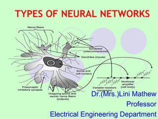
TYPES OF NEURAL NETWORKS
Dr.(Mrs.)Lini Mathew
Professor
Electrical Engineering Department

Simple Neural Network
X = I1W1+ I2W2+ ----- + INWN
Activation Function
S = K(X)
K is a threshold function
ie. S = 1 if X > T
S = O otherwise
T is a constant
threshold value.

Activation Functions
Threshold Function
S = 1 if X ≥ 0
S = 0 if X < 0
S = hardlim(X)
hard-limit transfer function
Also known as Heaviside step function
Binary-Step Function
S = 1 if X ≥ 
S = 0 if X < 
X
S
+1
-1
0
+1

Signum Function
S = 1 if X ≥ 0
S = -1 if X < 0
S = hardlims(X)
symmetric hard-limit transfer function
+1
X
S
-1
0
+1

Squashing Function or Logistic Function or Binary Sigmoidal
Function.
X = 0 S = 0.5 a is known
X > 0 S = 1 as steepness
X < 0 S = 0 parameter
S=logsig(X) log-sigmoid transfer function
aX
e
1
1
S 



Hyperbolic Tangent Function or Bipolar Sigmoidal Function
S = tanh(X)
X = 0 S = 0
X > 0 S = 1
X < 0 S = -1
S=tansig(X) tan-sigmoid transfer function
aX
-2aX
e
1
e
-
1
S 2
2
1
1
2






 aX
e

Linear Transfer Function
S = purelin(X)
also known as identity function
S=X for all X
Positive Linear Transfer Function
S = poslin(X)
S = X if X ≥ 0
S = 0 if X < 0
Transfer Functions - MATLAB
X
S
+1
-1
0
+1
S
X
+1
-1
0
+1

Saturating Linear Transfer Function
S = satlin(X)
S = X if 0 ≤ X ≤ 1
S = 0 if X < 0
S = 1 if X > 1
Symmetric Saturating Linear Transfer
Function
S = satlins(X)
S = X if -1 ≤ X ≤ 1
S = -1 if X < -1
S = 1 if X > 1
X
S
+1
-1
0
+1
+1
-1
X
S
+1
-1
0
+1
+1
-1

Radial Basis Function
S = radbas(X)
S=e−X
2
Triangular Basis Function
S = tribas(X)
S = 1-abs(X) if -1 ≤ X ≤ 1
S = 0 otherwise

McCulloch-Pitts Neuron Model
 Formulated by Warren McCulloch and Walter
Pitts in 1943
 McCulloch-Pitts neuron allows binary 0 or 1
states only ie.it is binary activated
 The input neurons are connected by direct
weighted path, excitatory or inhibitory
 The excitatory connections-positive weights,
inhibitory-negative weights
 Neuron is associated with a threshold value

Learning Rules
 A neural network learns about its environment through
an interactive process of adjustments applied to its
synaptic weights and bias levels.
 The set of well defined rules for the solution of a learning
problem is called a learning algorithm
 Hebbian Learning Rule. Oldest and most famous of all
learning rules, designed by Donald Hebb in 1949.
 Represents a purely feed-forward, unsupervised learning
 If the cross product of output and input is positive, this
results in increase of weights, otherwise the weight
decreases.
 The weights are adjusted as Wij
(k+1)
= Wij
(k)
+ xi y

Learning Rules
 Perceptron Learning Rule. Learning signal is the difference
between the desired and natural neuron’s response.
 This type of learning is supervised.
 Neti = b + Σxi Wi
Calculated output
yi = f(Neti) = 1 if Neti > 0
= 0 if -0 ≤ Neti ≤ 0
= -1 if Neti < -0
Weight updation
 If t ≠ y and the value of xi not equal to zero
Wi
(k+1)
= Wi
(k)
+ α t xi
bi
(k+1)
= bi
(k)
+ α t
 If t = y, there is no change in weights

Learning Rules
 Delta Learning Rule (Widrow-Hoff Rule or Least Mean
Square (LMS) Rule.
 The delta learning rule is valid only for continuous
activation functions and in the supervised training mode.
 The delta rule assumes that the error signal is directly
measurable.
 The aim of the delta rule is to minimize the error over all
training patterns.
 ∆Wi = α (t - yi) xi
 The mean square error for a particular pattern is
E = Σ(ti – yi)2
 The gradient of E is a vector consisting of partial
derivatives of E with respect to each of the weights.

Learning Rules
 Competitive Learning Rule.
 This rule has a mechanism that permits the neurons to
compete for the right to respond to a given subset of
inputs, such that only one output neuron per group is
active at a time.
 The winner neuron during competition is called winner-
takes-all neuron.
 This rule is suited for unsupervised network training. This
is the standard Kohenen learning rule.
 For neuron P to be the winning neuron, its induced local
field vp for a given particular input pattern must be largest
among all the neurons in the network.
N = 1 if vp > vq for all q, p ≠ q
N = 0 otherwise

Characteristics of Neural Networks
 Exhibit mapping capabilities. They can map input
patterns to their associated output patterns
 Learn by examples. They can be trained with
known examples of a problem and therefore can
identify new objects previously untrained
 Possess the capability to generalize. They can
predict new outcomes from past trends.
 Are robust systems and are fault tolerant. They
can recall full patterns from incomplete, partial or
noisy patterns.
 Can process information in parallel, at high speed
and in a distributed manner

Single Layer Perceptron - The simplest form
of neural network used for the classification
of patterns that are linearly separable.
Algorithm – To start the training process,
initially the weights and biases are set to
zero.
The learning rate value is set, which ranges
from 0 to 1.
Wi
(k+1)
= Wi
(k)
+ α t xi
bi
(k+1)
= bi
(k)
+ α t
Perceptron Network

Example: Training of an AND gate
(i) Bias b = 0 W1
(0)
= 0 W2
(0)
=0
Neti = b + Σxi Wi Net1 = 0 + 0 = 0
y1 = 0 as Net1 = 0 t = -1
W1
(1)
= W1
(0)
+  t x1 = 0 + 1x-1x-1 = 1
W2
(1)
= W2
(0)
+  t x2 = 0 + 1x-1x-1 = 1
b
(1)
= b
(0)
+ α t = 0 + 1x-1 = -1
Perceptron
x1 x2 t
0 0 0
0 1 0
1 0 0
1 1 1
x1 x2 t
-1 -1 -1
-1 1 -1
1 -1 -1
1 1 1

(ii) b = -1 W1
(1)
= 1 W2
(1)
= 1 x1 = -1 x2 = 1
Net1 = -1 + 1x-1 + 1x1 = -1
y1 = -1 as Net1 < 0 t = -1
No weight change
(iii) b = -1 W1
(1)
= 1 W2
(1)
= 1 x1 = 1 x2 = -1
Net1 = -1 + 1x1 + 1x-1 = -1
y1 = -1 as Net1 < 0 t = -1
No weight change
Perceptron

(iv) b = -1 W1
(1)
= 1 W2
(1)
= 1 x1 = 1 x2 = 1
Net1 = -1 + 1x1 + 1x1 = 1
y1 = 1 as Net1 > 0 t = 1
No weight change
Epoch 2
Perceptron
x1 x2 b net y t w1 w2
-1 -1 -1 -3 -1 -1 1 1
-1 1 -1 -1 -1 -1 1 1
1 -1 -1 -1 -1 -1 1 1
1 1 -1 1 1 1 1 1

Linear Separability
(0,0) (0,1)
(1,0) (1,1)
AND
(0,0) (0,1)
(1,0) (1,1)
XOR

Linear Separability
 Netj = Σ xi wi + b = x1 w1 + x2 w2 + b
 The relation Σ xi wi + b = 0 gives the boundary region of
the net input.
 The equation denoting this decision boundary can
represent a line or plane.
 On training, if the weights of training input vectors of
correct response +1 lie on one side of the boundary and
that of -1 lie on the other side of the boundary, then the
problem is linearly separable.
 x1 w1 + x2 w2 + b = 0
2
1
1
2
2
w
w
x
w
b
x 



-0.8 -0.6 -0.4 -0.2 0 0.2 0.4 0.6
-1
-0.5
0
0.5
1
1.5
Vectors to be Classified
P(1)
P(2)
-0.8 -0.6 -0.4 -0.2 0 0.2 0.4 0.6
-1
-0.5
0
0.5
1
1.5
Vectors to be Classified
P(1)
P(2)
Linear Separability

Linear Separability
(0,0) (0,1)
(1,0) (1,1)
XOR
(0,0) (0,1)
(1,0) (1,1)
AND
Perceptrons are successful only on problems
with linearly separable solution space.

ADALINE Network
 Adaptive Linear Neuron
 Developed by Widrow and Hoff in 1960.
 Inputs could be binary, bipolar or real valued
 The training process is continued until the error
(t-yi) is minimum.
 Mean Square Error 𝐸 = 𝑖=1
𝑛
(𝑡 − 𝑦𝑖)2
 Learning algorithm (Delta Rule)
yi = 1 if Neti ≥ 0
= -1 otherwise
Weight Adjustment:
Wi
(k+1)
= Wi
(k)
+  (t-yi)xi

Example: ADALINE network for OR function
(i) Bias b = w1
(0)
= w2
(0)
= 0.1  = 0.4
Neti = b + Σxi wi Net1 = 0.1 + 0.1 +0.1 = 0.3
y1 = 0.3 t = 1 ∆wi = α(t - yi)xi
w1
(1)
= w1
(0)
+ ∆w1 = 0.1 + 0.4x0.7x1 = 0.38
w2
(1)
= w2
(0)
+ ∆w2 = 0.1 + 0.4x0.7x1 = 0.38
b
(1)
= b
(0)
+ α(t - yi) = 0.1 + 0.4x0.7 = 0.38
ADALINE Network
x1 x2 t
1 1 1
1 -1 1
-1 1 1
-1 -1 -1
Activation function is
Identity Function.
yi = neti

Epoch 1 : b = w1
(0)
= w2
(0)
= 0.38  = 0.4
∆w2 = 0.4x(1–0.38)x1 = 0.248 w1
(1)
= 0.38-0.25 = 0.13
w2
(1)
= 0.38+0.25 = 0.63 ∆w3= 0.4x(1–0.13)x1 = 0.348
∆w4 = 0.4x(-1–0.22)x-1 = 0.488
E = ∑ (t-y)2 = 0.49 + 0.38 + 0.76 + 1.49 = 3.12
ADALINE Network
x1 x2 b y t dw1 dw2 db w1 w2 b (t-y)2
1 1 1 0.3 1 0.28 0.28 0.28 0.38 0.38 0.38 0.49
1 -1 1 0.38 1 0.25 -0.25 0.25 0.63 0.13 0.63 0.38
-1 1 1 0.13 1 -0.35 0.35 0.35 0.28 0.48 0.98 0.76
-1 -1 1 0.22 -1 0.49 0.49 -0.49 0.77 0.97 0.49 1.49

Epoch 2 : b = 0.49 w1
(0)
= 0.77 w2
(0)
= 0.97  = 0.4
∆w2 = 0.4x(1–2.23)x1 = 0.492 w1
(1)
= 0.77-0.49 = 0.28
w2
(1)
= 0.97-0.49 = 0.48 ∆w3= 0.4x(1+0.2)x1 = 0.48
∆w4 = 0.4x(1+0.28)x1 = 0.51
∆w4 = 0.4x(-1-0.23)x-1 = 0.49
E = ∑ (t-y)2 = 1.51+ 1.44 + 1.64 + 1.51 = 6.1
ADALINE Network
x1 x2 b y t dw1 dw2 db w1 w2 b (t-y)2
1 1 1 2.23 1 -0.49 -0.49 -0.49 0.28 0.48 0 1.51
1 -1 1 -0.2 1 0.48 -0.48 0.48 0.76 0 0.48 1.44
-1 1 1 -0.28 1 -0.51 0.51 0.51 0.25 0.51 0.99 1.64
-1 -1 1 0.23 -1 0.49 0.49 -0.49 0.74 1.0 0.5 1.51

MADALINE Network
Developed by Bernard Widrow
Multiple ADALINE Network
Combining a number of ADALINE Networks
spread across multiple layers with adjustable
weights
The use of multiple ADALINEs help counter
the problem of non-linear separability

Perceptron Learning Functions
in MATLAB
learnp
 learnp is the perceptron weight/bias learning function.
 learnp calculates the weight change dW for a given neuron
from the neuron's input P and error E according to the
perceptron learning rule:
 dw = 0, if e = 0
= p', if e = 1
= -p', e = -1
 This can be summarized as
 dw = e*p

Perceptron Learning Functions
learnpn
 Normalized perceptron weight and bias learning function
 learnpn is a weight and bias learning function. It can result
in faster learning than learnp when input vectors have
widely varying magnitudes.
 learnpn calculates the weight change dW for a given neuron
from the neuron's input P and error E according to the
normalized perceptron learning rule:
 pn = p / sqrt(1 + p(1)^2 + p(2)^2) + ... + p(R)^2)
 dw = 0, if e = 0
= pn', if e = 1
= -pn', if e = -1
 The expression for dW can be summarized as
dw = e*pn'

Multilayer Perceptron (MLP)
 The oldest and most popular multi-layer neural network
architectures
 Use a non-linear activation function like the logistic
sigmoid or the hyperbolic tangent, or a piecewise-linear
activation function such as Rectifier Linear Unit (ReLU).

Multilayer Perceptron
 The advantage of the MLP over the classic
Perceptron and Adaline.
 Can create complex, non-linear decision boundaries
that allow us to tackle problems where the different
classes are not linearly separable.

Back Propagation Network
Developed by Rumelhart, Hinton, Williams
The Back propagation learning rule is
applicable on any feed forward network
architecture (multilayer also)
The Back propagation is a systematic method
of training, built on high mathematical
foundation and has very good application
potential.
BP algorithm is a generalization of the Delta
rule or Widrow-Hoff error correction rule.
Slow rate of convergence and local minima
problem are its weaknesses

Error Back Propagation
 The Back propagation learning rule is applicable on
any multilayer feed forward network architecture.
 It can be considered the cornerstone of modern
neural networks and deep learning.
 The backpropagation algorithm consists of two
steps:
Forward Pass: inputs pass through the network and
receive output predictions (this step is also known as
the propagation step).
Backward Pass: the loss function gradient is
calculated in the network's final layer (prediction
layer). It is used then for recursive application of the
chain rule to update the weights in the network (also
known as weight update or backpropagation)

 The input array x passes through the first layer,
whose output values are connected to the input
values of the next layer, and so on, until the
network gives, the outputs of the last layer.
 Calculate the value of the error function,
obtained by comparison with the expected output
value.
 In order to minimize the error, the gradients of
the error function with respect to each weight is
calculated.

 Since the gradient vector has been calculated, each
weight is updated in an iterative way, and
recalculating the gradients at the beginning of each
training iteration step, until the error becomes lower
than a certain established threshold, or the
maximum number of iterations is reached, when
finally the algorithm ends, the network is well trained.
 Current deep learning networks, like Convolutional
Neural Networks, also uses backpropagation
internally.
 Recurrent Neural Networks, which has been used for
natural language processing, also utilizes this
algorithm.

Ii1
Ii2
Ii3
Oi1
Oi2
Oi3
Ih1
Ih2
Ih3
Oh1
Oh2
Oh3
Io1
Io2
Io3
Oo1
Oo2
Oo3
V11
V21
V12
V22
V32
V13
V23
V33
V31
W11
W21
W31

Input Layer Computation
{O}i = {I}I
{I}h = [V]t {O}i
Hidden Layer Computation
{I}o = [W]t {O}h
   







 
 h
h f
I
h
e
O 
1
1  sigmoidal gain
fh threshold of
the hidden layer

Output Layer Computation
Calculation of error (Euclidean Norm)
   







 
 o
o f
I
o
e
O 
1
1
 
 

2
2
1
o
o O
T
E

MLFF networks with non-linear activation functions
have MSE surface above the total Q-dimensional space
which is not a smooth parabolic surface.
The error surface is complex and consists of many local
and global minima.
V
W
E
A
B
Initial weights
adjusted weights
best weights
C

 During training, the incremental adjustments to
the weights have been made, the location is
shifted to a different E location on the error-
weight surface.
 In moving down the error-weight surface, the
path followed depends on the shape of the
surface and the learning rate.
 The error surface is assumed to be truly
spherical
Vector AB = (Vi+1 - Vi)ī + (Wi+1 - Wi)ĵ = Vī + Wĵ












 j
W
E
i
V
E
AB 

 
 
   
W
E
W
O
O
O
O
T
W
E
O
W
I
O
O
I
O
O
T
O
E
W
I
I
O
O
E
W
E
h
o
o
o
h
O
o
o
O
O
o
O
o
o
o
o



































1
1

   







 
 o
o f
I
o
e
O 
1
1
   
    





























2
2
1
1 o
o
o
o
I
I
I
I
o
o e
e
e
e
O
dI
d






 
 
 
    








































 2
1
1
1
1
1
1
1
o
o
o
o
o I
I
I
I
I
o
o
e
e
e
e
e
O
O









     
i
i
i
i
i
i
i
i
i
i
i
h
h
o
o
o
o
o
h
h
o
o
o
o
V
V
V
W
W
W
V
V
E
V
W
W
E
W
V
E
V
I
O
O
W
O
O
O
T
V
E
V
I
I
O
O
I
I
O
O
E
V
E

















































1
1
1
1
1
1








 Learning Rate Coefficient (α)
 Determines the size of the weight adjustments
made at each iteration and hence influences
the rate of convergence.
 Momentum Term (Coefficient): (η)
 Momentum is used to keep the training process
going in the same general direction.
 ie. By adding a fraction of the previous weight
change to the current weight change.
 It reduces the training time and enhances the
stability of the training process.

weight matrices
V =
W =
Back Propagation Example
x1 x2 T
0.4 -0.7 0.1
0.3 -0.5 0.05
0.6 0.1 0.3
0.2 0.4 0.25
0.4
-0.7
Oi2
0.1
-0.2
0.4
0.2
0.2
-0.5
0.1 0.4
-0.2 0.2
0.2
-0.5

Back Propagation Example
Oi = Ii = V =
Ih = Vt Oi = =
Oh =
Io = Wt Oh = = -0.14354
Oo = 0.4642 and T = 0.1
E = (0.1 – 0.4642)2 = 0.13264
0.2 -0.5
0.4
-0.7
0.1 -0.2
0.4 0.2
0.4
-0.7
0.18
0.02
0.5448
0.505
0.5448
0.505
0.1 0.4
-0.2 0.2

( ) ( ) h
o
o
o O
O
-
1
O
O
-
T
λ
=
W
E
∂
∂
= 1*(0.1-0.4642)*0.4642*(1-0.4642)*
= -0.09058 *
=
( ) ( ) ( ) i
h
h
o
o
o I
O
-
1
O
Wλ
O
-
1
O
O
-
T
λ
=
V
E
∂
∂
0.5448
0.505
-0.0493
-0.0457
0.5448
0.505

= -0.09058* * * *Oi
=
=
( ) ( ) ( ) i
h
h
o
o
o O
O
-
1
O
Wλ
O
-
1
O
O
-
T
λ
=
V
E
∂
∂
1- 0.5448
1- 0.505
-0.00449 0.01132
0.5448
0.505
0.2
-0.5
0.4
-0.7
-0.001077 0.002716
0.001855 0.004754

Gradient Descent Training Functions
traingd
 Gradient descent backpropagation
 traingd can train any network as long as its weight, net input, and
transfer functions have derivative functions.
 Backpropagation is used to calculate derivatives of performance
perf with respect to the weight and bias variables X. Each variable
is adjusted according to gradient descent:
dX = lr * dperf/dX
traingdm
 Gradient descent with momentum backpropagation
perf with respect to the weight and bias variables X. Each variable
is adjusted according to gradient descent with momentum,
dX = mc*dXprev + lr*(1-mc)*dperf/dX
where dXprev is the previous change to the weight or bias.

traingda
 Gradient descent with adaptive learning rate backpropagation
 traingda can train any network as long as its weight, net
input, and transfer functions have derivative functions.
 Backpropagation is used to calculate derivatives of
performance perf with respect to the weight and bias
variables X.
 Each variable is adjusted according to gradient descent:
dX = lr * dperf/dX
At each epoch, if performance decreases toward the goal,
then the learning rate is increased by the factor lr_inc.
If performance increases by more than the factor
max_perf_inc, the learning rate is adjusted by the factor
lr_dec and the change that increased the performance is not
made.

traingdx
 Gradient descent with momentum and adaptive learning rate
backpropagation
 traingdx can train any network as long as its weight, net input, and
transfer functions have derivative functions.
perf with respect to the weight and bias variables X.
 Each variable is adjusted according to gradient descent with
momentum,
dX = mc*dXprev + lr*mc*dperf/dX
where dXprev is the previous change to the weight or bias.
For each epoch, if performance decreases toward the goal, then
the learning rate is increased by the factor lr_inc.
If performance increases by more than the factor max_perf_inc, the
learning rate is adjusted by the factor lr_dec and the change that
increased the performance is not made.

Gradient Descent Learning Functions
learngd
 learngd is the gradient descent weight and bias learning function.
 learngd calculates the weight change dW for a given neuron from
the neuron's input P and error E, and the weight (or bias) learning
rate lr, according to the gradient descent dW = lr*gW.
learngdm
 learngdm is the gradient descent with momentum weight and bias
learning function.
 learngdm calculates the weight change dW for a given neuron
from the neuron's input P and error E, the weight (or bias) W,
learning rate lr, and momentum constant mc, according to
gradient descent with momentum:
dW = mc*dWprev + (1-mc)*lr*gW
 The previous weight change dWprev is stored and read from the
learning state LS.

Associative Memory
Developed by John Hopfield
Single layer feed forward or recurrent
network which makes use of Hebbian
learning or Gradient Descent learning rule
A storehouse of associated patterns
A content-addressable memory system
allows the recall of data on the degree of
similarity between the input patterns and
the patterns stored in memory.
Associative Memory Neural Networks
(AMNN) -

Associative Memory
AMNN – Hopfield Neural Networks and
Bi-directional Associative Memory.
AMNN are single layer networks in which
the weights are determined for the
network to store a set of pattern
associations. Each association is an
input-output vector pair
AutoAMNN – if the input vector is same
as that of the output vector associated
HeteroAMNN – if inputs and outputs are
different

Auto Associative Memory
 Hopfield Associative Memory
 Connection matrix is indicative of the association of
the pattern with itself
 Autocorrelator’s recall
equation (activation function)
 Two parameter bipolar
threshold equation
 Hamming Distance of
vector X from Y
  
i
m
i
T
i A
A
T 


1
( )
( )
0
<
α
1
-
0
=
α
β
0
>
α
1
=
β
α
=
if
if
if
f
a
t
a
f
a old
j
ij
i
new
j
,
,
,
,
,
  



n
i
i
i y
x
y
x
HD
1
,

Auto Associative Memory - Example
Considering three patterns
A1 =
A2 =
A3 =
Recall Equation
T =
-1 1 -1 1
1 1 1 -1
-1 -1 -1 1
  
i
m
i
T
i A
A
T 


1
3 1 3 -3
1 3 1 -1
3 1 3 -3
-3 -1 -3 3
 
 










0
,
1
-
0
,
0
,
1
,
,






if
if
if
f
a
t
a
f
a old
j
ij
i
new
j

Stored pattern A2 = T =
a1
new
= f(1x3 + 1x1 + 1x3 + -1x-3, 1)
= f(3+1+3+3, 1)
= f(10, 1) = 1
a2
new
= f(6, 1) = 1
a3
new
= f(10, 1) = 1
a4
new
= f(-10, -1) = -1
A2
new =
1 1 1 -1 3 1 3 -3
1 3 1 -1
3 1 3 -3
-3 -1 -3 3
 
 










0
,
1
-
0
,
0
,
1
,
,






if
if
if
f
a
t
a
f
a old
j
ij
i
new
j
1 1 1 -1

Another noisy vector A’ =
a1
new
= f(3+1+3-3, 1)
= f(4, 1) = 1
a2
new
= f(4, 1) = 1
a3
new
= f(4, 1) = 1
a4
new
= f(-4, 1) = -1
A2
new =
1 1 1 1
 
 










0
,
1
-
0
,
0
,
1
,
,






if
if
if
f
a
t
a
f
a old
j
ij
i
new
j
1 1 1 -1

Hetero Associative Memory
 Developed by Bart Kosko
 Hetero Associative memory neural network
consists of only one layer of weighted
interconnections.
 There exists ‘n’ number of input neurons in the
input layer and ‘m’ number of output neurons in
the output layer.
 This is a fully interconnected network, wherein the
inputs and the outputs are different, hence it is
called Hetero Associative memory neural network.
 The weights are found using the Hebb Rule

 There are N training pairs {(A1,B1), (A2,B2),--- }
 Ai = (ai1, ai2, ai3 …….. ain)
 Bi = (bi1, bi2, bi3 …….. bin)
 Correlation Matrix
 Bi-directional Associative Memory (BAM) is a
hetero associative recurrent neural network
consisting of two layers.
 The net iterates by sending a signal back and
forth between the two layers until each neuron’s
activation remains constant for several steps.
[ ][ ]
i
m
1
=
i
T
i B
A
=
M ∑

The net can respond to input on either layer.
The layers are referred to as X-layer and Y-
layer instead of input and output layer.
B’ = f(AM)
A’ = f(B’MT
) Recall Equation
B’’ = f(A’M)
A’’ = f(B’’MT
)
 









0
,
1
-
0
,
0
,
1
,






if
if
if
f

A1 = B1 =
A2 = B2 =
A3 = B3 =
Converting to bipolar
A1 = B1 =
A2 = B2 =
A3 = B3 =
1 0 0 1
1 0 1 0
1 1 0 0
1 0 1
0 1 1
0 0 1
1 -1 -1 1 1 -1 1
-1 -1 1
1 -1 1 -1
1 1 -1 -1
-1 1 1
Bi-directional Associative Memories

Finding the connection matrix
M = + +
M =   
i
m
i
T
i B
A
M 


1
-1 -1 3
-1 -1 -1
-1 3 -1
3 -1 -1
1 -1 1
1
-1
-1
1
-1 1 1
1
-1
1
-1
-1 -1 1
1
1
-1
-1

Stored pattern A1 = M =
b1
new
= f(1x-1 +-1x-1 +-1x-1 + 1x3, 1)
= f(-1+1+1+3, 1)
= f(4, 1) = 1
b2
new
= f(-4, 1) = -1
b3
new
= f(4, 1) = 1
B1
new =
1 -1 -1 1
1 -1 1
-1 -1 3
-1 -1 -1
-1 3 -1
3 -1 -1
 









0
,
1
-
0
,
0
,
1
,






if
if
if
f

with pattern B1 = MT =
a1
new
= f(1x-1 + -1x-1 + 1x3, 1)
= f(-1+1+3, 1)
= f(3, 1) = 1
a2
new
= f(-1, 1) = -1
a3
new
= f(-4, 1) = -1
a4
new
= f(3, 1) = 1
A1
new =
-1 -1 -1 3
-1 -1 3 -1
3 -1 -1 -1
1 -1 1
1 -1 -1 1
 









0
,
1
-
0
,
0
,
1
,






if
if
if
f

Two stored patterns of letter E
Connection matrix
Character Recognition
1 1 1
1 0 0
1 1 1
1 0 0
1 1 1
1 1 1
1 0 0
1 1 0
1 0 0
1 1 1
1 1 1
1 -1 -1
1 1 1
1 -1 -1
1 1 1
1 1 1
1 -1 -1
1 1 -1
1 -1 -1
1 1 1
10 2 0
2 10 8
0 8 10

Two stored patterns of letter E
Connection matrix will be a 15x15 matrix
Character Recognition
1 1 1 1 -1 -1 1 1 1 1 -1 -1 1 1 1
1 1 1 1 -1 -1 1 1 -1 1 -1 -1 1 1 1

Self-Organizing Maps (SOMs)
 Self-Organizing Maps (SOMs)
were invented by Professor T.
Kohenen. Also known as
Kohenen Neural Netwok (KNN)
 This topology uses an
unsupervised learning procedure
to produce a two-dimensional
discretized representation of the
input space of the training
samples called a ‘map’.
 KNN is widely used for clustering
applications
Competitive Network

 Kohenen worked in the development of the theory
of competition.
 The mostly used competition among group of
neurons is Winner-Takes-All.
 Here, only one neuron in the competing group will
have a non-zero output signal when the
competition is completed.
 The self-organizing map, developed by Kohenen,
groups the input data into clusters which are
commonly used for unsupervised learning.

 Whenever an input is presented, the network
finds out the “distance” of the weight vector of
each node from the input vector, and selects the
node with the greatest distance.
 In this way, the whole network selects the node
with its weight vector closest to the input vector,
i.e. the winner.
 The network learns by moving the winning
weight vector towards the input vector while the
other weight vectors remain unchanged

 If the samples are in clusters, then every time
the winning weight vector moves towards a
particular sample in one of the clusters.
 Eventually each of the weight vectors would
converge to the centroid of one cluster. At this
point, the training is complete.
 After training, the weight vectors become
centroids of various clusters.

 To cluster 4 bipolar input patterns into 2 clusters.
 I1 = [1 1 1 -1]
 I2 = [-1 -1 -1 1]
 I3 = [1 -1 -1 -1]
 I4 = [-1 -1 1 1]
 The weights connected to the cluster units are:
 W1 = [0.2 0.6 0.5 0.9]
 W2 = [0.8 0.4 0.7 0.3]
 Learning rate α = 0.9
Clustering of Bipolar Input Patterns

 Euclidean Distance (ED) between the weight
vector associated with it and the given input
vector is the minimum
 ED(1)= 𝑖=1:𝑛 𝑊𝑖 − 𝐼𝑖
2
 ED(1) = (0.2-1)2+(0.6-1)2+(0.5-1)2+(0.9-(-1))2
= 4.66
 ED(2) = (0.8-1)2+(0.4-1)2+(0.7-1)2+(0.3-(-1))2
= 2.18
 Winner is the second cluster unit as ED is
minimum

 Weight Updation for cluster 2
 Wi=2(new) = Wi=2(old) + α*(I1 - Wi=2(old))
 W2 = [0.8 0.4 0.7 0.3]
 W21(new) = 0.8 + 0.9*(1-0.8) = 0.98
 W22(new) = 0.4 + 0.9*(1-0.4) = 0.94
 W23(new) = 0.7 + 0.9*(1-0.7) = 0.97
 W24(new) = 0.3 + 0.9*(-1-0.3) = -0.87
 W2(new) = [0.98 0.94 0.97 -0.87]
 W1 = [0.2 0.6 0.5 0.9]



 W1 = [0.2 0.6 0.5 0.9]
 W11(new) = 0.2 + 0.9*(-1-0.2) = -0.88
 W12(new) = 0.6 + 0.9*(-1-0.6) = -0.84
 W13(new) = 0.5 + 0.9*(-1-0.5) = -0.85
 W14(new) = 0.9 + 0.9*(1-0.9) = 0.99
 W1(new) = [-0.88 -0.84 -0.85 0.99]
 W2(new) = [0.98 0.94 0.97 -0.87]

 W1 = [-0.88 -0.84 -0.85 0.99]
 W11(new) = -0.88 + 0.9*(1-(-0.88)) = 0.812
 W12(new) = -0.84 + 0.9*(-1-(-0.84)) = -0.984
 W13(new) = -0.85 + 0.9*(-1-(-0.85)) = -0.985
 W14(new) = 0.99 + 0.9*(-1-0.99) = -0.801
 W1(new) = [0.812 -0.984 -0.985 -0.801]
 W2(new) = [0.98 0.94 0.97 -0.87]

 Euclidean Distance (ED) for pattern 4
I4 = [-1 -1 1 1]
 ED(1)= 𝑖=1:𝑛 𝑊𝑖 − 𝐼𝑖
2
 ED(1) = (0.812-(-1)2+(-0.984-(-1))2+(-0.985-1)2
+(-0.801-1)2 = 10.4674
 ED(2) = (0.98-(-1))2+(0.94-(-1))2+(0.97-1)2
+(-0.87-1)2 = 11.1818
 Winner is the first cluster unit as ED is minimum

 W1(new) = [0.812 -0.984 -0.985 -0.801]
 W11(new) = 0.812 + 0.9*(-1- 0.812) = -0.8188
 W12(new) = -0.984 + 0.9*(-1-(-0.984)) = -0.9984
 W13(new) = -0.985 + 0.9*(1-(-0.985)) = 0.8015
 W14(new) = -0.801 + 0.9*(1-(-0.801)) = 0.8199
 W1(new) = [-0.8188 -0.9984 -0.8015 0.8199]
 W2(new) = [0.98 0.94 0.97 -0.87]
 After one epoch (iteration), patterns I2,I3 and I4 are
in cluster W1 and I1 is in cluster W2
 After several epochs, clustering becomes stagnant

Clustering Technique
Vector Quantization is a method of dynamic
allocation of cluster centers.
To begin with, the first pattern will create the
cluster to hold it.
Points x y Points x y
P1 2 3 P7 6 4
P2 3 3 P8 7 4
P3 2 6 P9 2 4
P4 3 6 P10 3 4
P5 6 3 P11 2 7
P6 7 3 P12 3 7

0
1
2
3
4
5
6
7
8
0 1 2 3 4 5 6 7 8
P1
P9
P11
P4
P12
P5
P7
P6
P8
P3
P2
P10

0
1
2
3
4
5
6
7
8
0 1 2 3 4 5 6 7 8
C1
C3
C2

Coordinates of P1 = (2,3)
Centre of Cluster C1 = (2,3)
Threshold distance = 1.5
Considering point P2 whose coordinates are (3,3)
Distance between P2 and C1 =((3-2)2 + (3-3)2) = 1.0 < 1.5
Hence P2 is included in C1
New cluster centre of C1 =
3+2
2
,
3+3
2
= (2.5, 3)
Points x y Points x y
P1 2 3 P7 6 4
P2 3 3 P8 7 4
P3 2 6 P9 2 4
P4 3 6 P10 3 4
P5 6 3 P11 2 7
P6 7 3 P12 3 7

0
1
2
3
4
5
6
7
8
0 1 2 3 4 5 6 7 8
C1
P1
P9
P11
P4
P12
P5
P7
P6
P8
P3
P2
P10

Centre of Cluster C1 = (2.5,3)
Distance between P3 and C1 =((2-2.5)2 + (6-3)2) = 3.04
This is greater than 1.5
Hence P3 is not included in C1.
Another cluster C2 is selected whose centre is (2, 6)
Distance between P4 and C1 =((3-2.5)2 + (6-3)2) = 3.04 > 1.5
Hence P4 is not included in C1 but included in C2
3+2
2
,
6+6
2
= (2.5, 6)

0
1
2
3
4
5
6
7
8
0 1 2 3 4 5 6 7 8
C1
P1
P9
P11
P4
P12
P5
P7
P6
P8
C2
P3
P2
P10

Hence P5 is not included in C1 and also in C2
Another cluster C3 is selected whose centre is (6, 3)
Hence P6 is not included in C1 and in C2
Now P6 is included in C3
6+7
2
,
3+3
2
= (6.5, 3)

0
1
2
3
4
5
6
7
8
0 1 2 3 4 5 6 7 8
C1
P1
P9
P11
P4
P12
P5
P7
P6
P8
C2
C3
P3
P2
P10

Adaptive Resonance Theory
 ART was introduced by Carpenter and Stephen
Grossberg
 Widely used for clustering applications.
 The problems faced by competitive NNs are that
they do not always form stable clusters.
 They are oscillatory when more input patterns are
presented.
 ART NN are receptive to significant new patterns
and still remains stable.
 There are three types of ART networks: (i) ART-1
(ii) ART-2 and (iii) ART-3

 ART-1 can cluster only binary inputs
 ART-2 can handle gray-scale inputs
 ART-3 can handle analog inputs better by
overcoming the limitations of ART-2.
 The basic ART learning is an unsupervised one.
 Stability of the network means that a pattern
should not oscillate among different cluster units
at different stages of training.
 Plasticity is the ability of the net to respond to
learn new pattern equally well at any stage of
learning.

 The key innovation of ART is the use of a degree
of expectation called vigilance parameter.
 Vigilance parameter is the user specified value to
decide the degree of similarity essential for the
input patterns to be assigned to a cluster unit.
 As each input is presented to the network, it is
compared with the prototype vector for a match
based on the vigilance parameter.
 If the match is not adequate, a new prototype or a
cluster unit is selected.
 In this way, previous learned memories
(prototypes) are not eroded by new learning.

 ‘Resonance’ in ART is the state of the network
when a class of prototype vector very closely
matches to the current input vector, and leads to
a state which permits learning.
 During this resonant state, the weight updation
takes place.
 The basic architecture consists of three layers:
 Input Processing Layer for processing the given
inputs.
 Further divided into Input Layer and Input
Interface Layer
 Output layer has the cluster units. This is the
competitive layer or a recognition region.

 Interface layer is called the comparison region
where it transfers the input vector to its best
match in the recognition region.
 Reset Layer decides the degree of similarity of
patterns placed on the same cluster by a reset
mechanism.
 It compares the strength of the recognition match
to the vigilance parameter.
 Bottom-up weights are connected between the
Input Interface Layer to the Output layer.
 Top-down weights are connected between the
Output layer to the Input Interface Layer.

Output layer
Input layer
Reset layer Input Interface
layer
Bottom-up weights
Top-down weights

 The units transmit the information to the output
layer through the bottom-up weights u,
 O1 = I1u11 + I2u12 = 0.5*0.3 + 0.6*0.5 = 0.45
 O2 = I1u21 + I2u22 = 0.5*0.2 + 0.6*0.6 = 0.46
 O2 > O1 so output cluster 2 is selected as winner
 The information about the winner is sent from the
output layer to the interface layer through the top-
down weights d.
 I1 = S1d11 = 0.5*0.1 = 0.05
 I2 = S2d12 = 0.6*0.3 = 0.18
 Norm of I is 𝐼 = I1 + I2 = 0.05 +0.18 = 0.23
 The value of 𝐼 gives an estimate of the degree
of match

 The learning will occur only if the match is
acceptable to the value of vigilance parameter.
 The verdict for learning is carried out by
calculating the ratio of 𝐼 and 𝑆 .
 The updation of the weights is carried out if
Match Ratio 𝐼
𝑆 ≥ v
 𝐼
𝑆 = 0.23/1.1 = 0.209 < v (0.3)
 If 𝐼
𝑆 < v, then the current cluster unit is
rejected and inhibited.

 Again I1 and I2 is calculated for next cluster unit
 I1 = S1d21 = 0.5*0.6 = 0.3
 I2 = S2d22 = 0.6*0.1 = 0.06
 𝐼 = I1 + I2 = 0.3 +0.06 = 0.36
 𝐼
𝑆 = 0.36/1.1 = 0.327 > v (0.3)
 Cluster 2 is selected and S is assigned to it.
 The weights associated with it are updated.

 The top-down weights associated with cluster 2
are assigned the new calculated values I1 and I2
 d21 = I1 = 0.3
 d22 = I2 = 0.06
 The new bottom-up weights are calculated as:
 u21 =
𝐿∗𝐼1
𝐿−1+ 𝐼
=
4∗0.3
4−1+0.36
= 0.454
 u22 =
𝐿∗𝐼2
𝐿−1+ 𝐼
=
4∗0.06
4−1+0.36
= 0.091
 This procedure is repeated until a cluster unit is
accepted or all the units in the output layer are
inhibited.

 If all the units in the output layer are inhibited, a
decision has to be taken by the user.
 Reduce the value of the vigilance parameter
allowing less matched patterns to be placed
on the same cluster units which may be
inhibited during earlier learning trial.
 Addition of more number of cluster units.
 Specify the current input pattern as the one
that cannot be clustered.
The vigilance parameter v can have a value less
than 1
 L > 1

 plotpv - Plots perceptron input/target vectors
 plotpv(P,T) P is the matrix of input vectors
and T is the matrix of binary target vectors
 P = [ -0.5 -0.5 +0.3 -0.1; -0.5 +0.5 -0.5 +1.0];
 T = [1 1 0 0]; plotpv(P,T);
 plotpc - Plots classification line on perceptron
vector plot
 plotpc(W,B) W is the weight matrix and B is the
bias vector
July 16, 2023 116
Neural Network Toolbox

 newp Creates a perceptron
 net = newp(P,T,TF,LF)
P is the R x Q1 matrix of input vectors
T is the S x Q2 matrix of target vectors
TF is the transfer function (default = ‘hardlim')
LF is the Learning function (default = 'learnp')
 net.iw{1,1} = [-1.2 -0.5]; net.b{1} = 1;
plotpc(net.iw{1,1},net.b{1})
 adapt Allow neural network to change weights
and biases on inputs
July 16, 2023 117
(percpt)

 adapt Allow neural network to change weights
and biases on inputs
 This function calculates network outputs and errors
after each presentation of an input.
 [net,Y,E,tr] = adapt(net,P,T)
net is the Network
P Network inputs
T Network targets (default = zeros)
Y Network outputs
E Network errors
tr Training record (epoch and perf)
 net.adaptParam.passes
July 16, 2023 118

 sim Simulate neural network
 This function calculates network outputs and errors
after each presentation of an input.

net is the Network
P Network inputs
Y Network outputs
E Network errors
 [Y,E,perf] = sim(net,P,T)
perf Network performance
July 16, 2023 119

 newff Creates a feed-forward
backpropagation network
 net = newff(P,T,Si,Tfi)
P is the R x Q1 matrix of input vectors
T is the SN x Q2 matrix of target vectors
Si is the Size of the ith (hidden) layer
TFi is the transfer function of the ith layer
This function initializes its weights and biases. It also
sets the input, output data processing functions and
training functions to default values
July 16, 2023 120
(feedfrwd)

 train Train neural network
 This function trains a network net according to
net.trainFcn and net.trainParam..
 [net, tr,Y,E] = train(net,P,T)
net is the Network
P Network inputs
Y Network outputs
E Network errors
tr Training record (epoch and perf)
 net.trainParam.epochs
 net.trainParam.goal
July 16, 2023 121

 Two different styles of training.
 Incremental training - the weights and biases of
the network are updated each time an input is
presented to the network.
 In this case, the function adapt is used , and the
inputs and targets are presented as sequences.
P = {[1;2] [2;1] [2;3] [3;1]}; T = {4 5 7 7};
 Batch training - the weights and biases are only
updated after all the inputs are presented.
The function train can only perform
batch training.
July 16, 2023 122

 train applies the inputs to the new network,
calculates the outputs, compares them to the
associated targets, and calculates a mean square
error. If the error goal is met, or if the maximum
number of epochs is reached, the training is
stopped, and train returns the new network and a
training record. Otherwise train goes through
another epoch.
 train uses a matrix of concurrent vectors.
P = [1 2 2 3; 2 1 3 1]; T = [4 5 7 7];
July 16, 2023 123

 Create and train a FF network to evaluate the
following function:
 for -10 < x < 10
 Generate input-output training data
x=-10:0.5:10
y=(x^2-6.5)/(x^2+6.5);
 Create a feed forward neural network
net=newff(x,y,5,{‘tansig’,’tansig’},’traingd’)
 Train the network
net=train(net,x,y);
July 16, 2023 124
5
.
6
+
x
6.5
-
x
=
y 2
2
(feedfrwd1)

 Pre-processing and Post-processing Inputs and
Outputs
 Result in faster and efficient training of the network
 Pre- and Post-processing training data functions
are assigned automatically by network creation
functions like newff
 The function mapminmax scales inputs and outputs
so that they are in the range [-1 1]
 The normalized output is converted back to original
by using the function mapminmax with argument
reverse
July 16, 2023 125
(preprocs)

Types of Neural Networks Explained

Recommended

Recommended

More Related Content

Similar to Types of Neural Networks Explained

Similar to Types of Neural Networks Explained (20)

Recently uploaded

Recently uploaded (20)

Types of Neural Networks Explained