SlideShare a Scribd company logo
1 of 16
Section & Lesson #:
Pre-Requisite Lessons:
Complex Tools + Clear Teaching = Powerful Results
Hypothesis Testing: Central Tendency –
Normal (Compare 2+ Factors)
Six Sigma-Analyze – Lesson 18
An extension on a series about hypothesis testing, this lesson reviews the
ANOVA test as a central tendency measurement for normal dist.
Six Sigma-Analyze #17 – Hypothesis Testing: Central Tendency –
Normal (Compare 1:1)
Copyright © 2011-2019 by Matthew J. Hansen. All Rights Reserved. No part of this publication may be reproduced, stored in a retrieval system, or transmitted by any means
(electronic, mechanical, photographic, photocopying, recording or otherwise) without prior permission in writing by the author and/or publisher.
Why do we need hypothesis testing?
o Remember, our project goal is to resolve a problem by first building a transfer function.
• We don’t want to just alleviate symptoms, we want to resolve the root cause.
 Remember Hannah? We don’t want to alleviate the arthritis pain in her leg, but heal the strep throat.
• If we don’t know what the root cause is, then we need to build a transfer function.
 By building a transfer function, we can know what changes (improvements) should fix the root cause.
o Remember, the Transfer Function is defined as Y = f(X).
• This is described as “output response Y
is a function of one or more input X’s”.
• It’s part of the IPO flow model where we
described the IPO flow model as one or
more inputs feeding into a process that
transforms it to create a new output.
o How does a transfer function fit with hypothesis testing?
• Hypothesis testing tells us which X’s (inputs) are independently influencing the Y (output).
 When we reject a null hypothesis, we’re building evidence proving which X’s are “guilty” of driving the Y.
 We’ll compile all the evidence in the Improve phase of DMAIC and begin to fix those root causes.
Copyright © 2011-2019 by Matthew J. Hansen. All Rights Reserved. No part of this publication may be
reproduced, stored in a retrieval system, or transmitted by any means (electronic, mechanical, photographic,
photocopying, recording or otherwise) without prior permission in writing by the author and/or publisher.
Y = f(X)
Input (X) > Process > Output (Y)
Review Hypothesis Testing: 4 Step Process
o Remember, the 4 high-level steps for hypothesis testing begin/end with being practical:
o As the heart of hypothesis testing, steps 2 & 3 can be drilled to the following 6 steps:
Copyright © 2011-2019 by Matthew J. Hansen. All Rights Reserved. No part of this publication may be
reproduced, stored in a retrieval system, or transmitted by any means (electronic, mechanical, photographic,
photocopying, recording or otherwise) without prior permission in writing by the author and/or publisher.
3
Practical Statistical
Problem Problem
Solution Solution
 

Practical Problem
State the problem as a
practical Yes/No question.
 Statistical Problem
Convert the problem to an
analytical question identifying
the statistical tool/method.

Practical Solution
Interpret the analytical
answer in a practical way.
Statistical Solution
Interpret the results of the
hypothesis test with an
analytical answer.

1. Define the objective.
2. State the Null Hypothesis (H0) and Alternative Hypothesis (Ha).
3. Define the confidence (1-α) and power (beta or 1-β).
4. Collect the sample data.
5. Calculate the P-value.
6. Interpret the results: accept or reject the null hypothesis (H0).
Is the data type for both values discrete?
What are you measuring?
Is the data normal?
SpreadCentral Tendency
Compare 1:Standard
1 Proportion Test
Compare 1:1
2 Proportion Test
Compare 2+ Factors
Chi2 Test
Compare 1:Standard
1 Sample T Test
Compare 1:1
2 Sample T Test
or Paired T Test
Compare 2+ Factors
One-way ANOVA Test
Compare 1:Standard
1 Sample Wilcoxon
or 1 Sample Sign
Compare 1:1
Mann-Whitney Test
Compare 2+ Factors
Mood’s Median Test
or Kruskal-Wallis Test
Compare 1:Standard
1 Variance Test
Compare 1:1
2 Variance Test
Compare 2+ Factors
Test for Equal Variances
Yes No
Yes No
Proportions
Compare 1:1
Pearson Correlation
or Fitted Line Plot
Compare 2+ Factors
Multiple Regression or
General Linear Model
Is the data type for both values continuous?
Relationships
No Yes
Review Finding the Right Statistical Test
o What statistical test do I use for my hypothesis testing?
• The type of statistical test depends on the data to be tested, as described in the chart below:
Copyright © 2011-2019 by Matthew J. Hansen. All Rights Reserved. No part of this publication may be
reproduced, stored in a retrieval system, or transmitted by any means (electronic, mechanical, photographic,
photocopying, recording or otherwise) without prior permission in writing by the author and/or publisher.
4
Lesson
Current
Confidence Intervals (CI) Redefined
o Remember, confidence intervals (CI) are an estimated upper/lower range of the mean.
• The CI narrows when you add more samples:
• Remember, statistics are intended to help you make inferences about a population.
 A mean of 57 with a 95% confidence interval of 55 and 59 implies that although the sample mean is only
57, you can be 95% confident that the population mean will fall somewhere between 55 and 59.
• The first step in hypothesis testing is to define the objective by asking “is there a difference…”
 Statistical tests generally compare the different CIs between factors to see if a difference exists.
Copyright © 2011-2019 by Matthew J. Hansen. All Rights Reserved. No part of this publication may be
reproduced, stored in a retrieval system, or transmitted by any means (electronic, mechanical, photographic,
photocopying, recording or otherwise) without prior permission in writing by the author and/or publisher.
5
With fewer samples, the population
mean falls within a wide interval.
Add more samples and the population
mean falls in a more narrow interval.
With more samples, the more confident
(narrow) the mean interval becomes.
Factor A
Factor B
2.5 2.75 3.0 3.25 3.5
Large overlap indicates the population
mean may be the same for both
groups; therefore there is no difference
between them (high P-value).
N = 20
Factor A
Factor B
2.5 2.75 3.0 3.25 3.5
Small overlap indicates a smaller chance
the population mean may be the same for
both groups; therefore there is may be no
difference between them (small P-value).
N = 50
Factor A
Factor B
2.5 2.75 3.0 3.25 3.5
No overlap indicates the population
mean is different for both groups;
therefore there is a difference between
them (low or no P-value).
N = 100
One-Way ANOVA: Introduction
o When should I use it?
• To compare mean values for multiple factors.
o How do I find it in Minitab?
• Stat > ANOVA > One-Way…
o What are the inputs for the test?
Copyright © 2011-2019 by Matthew J. Hansen. All Rights Reserved. No part of this publication may be
reproduced, stored in a retrieval system, or transmitted by any means (electronic, mechanical, photographic,
photocopying, recording or otherwise) without prior permission in writing by the author and/or publisher.
6
Now
The column containing the continuous
data to test; it should represent the Y or
CTQ output being measured.
The factor having 2 or more discrete values that each defines
the set of values for which each mean will be analyzed.
Creates a visual display of 4 different charts used to analyze
the residuals created by the ANOVA.
One-Way ANOVA: Interpreting Results
o How do I interpret the ANOVA results?
• Below is an example of the output from an ANOVA test.
• We’ll separately explore each summary and detail portion.
Copyright © 2011-2019 by Matthew J. Hansen. All Rights Reserved. No part of this publication may be
reproduced, stored in a retrieval system, or transmitted by any means (electronic, mechanical, photographic,
photocopying, recording or otherwise) without prior permission in writing by the author and/or publisher.
7
Now
Summary:
This portion summarizes
the results of the test.
Details:
This portion lists the
detailed results of the test.
One-Way ANOVA: Summary Portion
o What does the summary portion of the ANOVA results mean?
o What values do I use to interpret these results?
• If P-value < α (0.05), statistical difference exists.
• High R-sq may mean “practical” difference exists.
Copyright © 2011-2019 by Matthew J. Hansen. All Rights Reserved. No part of this publication may be
reproduced, stored in a retrieval system, or transmitted by any means (electronic, mechanical, photographic,
photocopying, recording or otherwise) without prior permission in writing by the author and/or publisher.
8
NowSource DF SS MS F P
CategoryA 4 426446 106611 2.07 0.091
Error 95 4900934 51589
Total 99 5327380
S = 227.1 R-Sq = 8.00% R-Sq(adj) = 4.13%
Between
analysis
results
Within
analysis
results
Sources of
variation
Degrees of
Freedom per
Source
(# of unique
values – 1)
Sum of Squares
(variation) per
Source
Estimate of
variation from
each source
(Calc’d as SS/DF)
P valueF ratio
(MSBetween
)MSWithin
Unexplained
Variation
(equals 1σ)
% of variation in MetricA (Response)
explained by CategoryA (Factor)
(Cald’d as SSFactor / SSTotal)
One-Way ANOVA: Detail Portion
o What does the detailed portion of the ANOVA results mean?
o How do I interpret these results?
• Examine the difference in each unique value’s mean
to see it’s significant (probably confirmed by R-sq).
Copyright © 2011-2019 by Matthew J. Hansen. All Rights Reserved. No part of this publication may be
reproduced, stored in a retrieval system, or transmitted by any means (electronic, mechanical, photographic,
photocopying, recording or otherwise) without prior permission in writing by the author and/or publisher.
9
Now
Individual 95% CIs For Mean Based on Pooled StDev
Level N Mean StDev +---------+---------+---------+---------
Blue 14 524.9 182.5 (---------*---------)
Green 14 362.5 141.3 (---------*---------)
Red 19 559.0 226.4 (--------*-------)
White 30 557.3 240.9 (-----*------)
Yellow 23 539.2 270.0 (-------*-------)
+---------+---------+---------+---------
240 360 480 600
Factor’s
unique
values
Count for each
unique value
Means per
unique value
Std Deviation
per unique value
Illustration of
Confidence Intervals
per unique value
The amount of overlap in these
CIs are what affect the p-value.
One-Way ANOVA: Residuals Introduction
o What are residuals?
• They represent all the deviations for each data point.
• Remember, a deviation is the distance a data point is from the mean.
o Why are residuals used in an ANOVA test?
• They help identify potential serious problems in the analysis.
• It helps validate the ANOVA test to ensure the results are reliable.
o What do we look for in the residuals?
• Residuals should have these characteristics:
 They should be normally distributed.
 They should be independent.
 They should have equal variances.
o How do I measure the residuals?
• In the ANOVA dialog box, select “Graphs…”.
• In the Graphs box, select “Four in One” from
the “Residual Plots” section (example at right).
Copyright © 2011-2019 by Matthew J. Hansen. All Rights Reserved. No part of this publication may be
reproduced, stored in a retrieval system, or transmitted by any means (electronic, mechanical, photographic,
photocopying, recording or otherwise) without prior permission in writing by the author and/or publisher.
10
Now
Deviation = 9 – 5 = 4
8004000-400-800
99.9
99
90
50
10
1
0.1
Residual
Percent
550500450400350
500
250
0
-250
-500
Fitted Value
Residual
6004002000-200-400
20
15
10
5
0
Residual
Frequency
1009080706050403020101
500
250
0
-250
-500
Observation Order
Residual
Normal Probability Plot Versus Fits
Histogram Versus Order
Residual Plots for MetricA
One-Way ANOVA: Residuals Interpretation
o Interpreting the residual plots for normality:
• These plotted residuals should be normally distributed.
Copyright © 2011-2019 by Matthew J. Hansen. All Rights Reserved. No part of this publication may be
reproduced, stored in a retrieval system, or transmitted by any means (electronic, mechanical, photographic,
photocopying, recording or otherwise) without prior permission in writing by the author and/or publisher.
11
Now
8004000-400-800
99.9
99
90
50
10
1
0.1
Residual
Percent
550500450400350
500
250
0
-250
-500
Fitted Value
Residual
6004002000-200-400
20
15
10
5
0
Residual
Frequency
1009080706050403020101
500
250
0
-250
-500
Observation Order
Residual
Normal Probability Plot Versus Fits
Histogram Versus Order
Residual Plots for MetricA
Though there’s no Anderson-
Darling test, these distributions
should still appear to be normal.
One-Way ANOVA: Residuals Interpretation
o Interpreting the residual plots for equal variance and independence:
• These plotted residuals should appear random yet evenly spread.
Copyright © 2011-2019 by Matthew J. Hansen. All Rights Reserved. No part of this publication may be
reproduced, stored in a retrieval system, or transmitted by any means (electronic, mechanical, photographic,
photocopying, recording or otherwise) without prior permission in writing by the author and/or publisher.
12
Now
8004000-400-800
99.9
99
90
50
10
1
0.1
Residual
Percent
550500450400350
500
250
0
-250
-500
Fitted Value
Residual
6004002000-200-400
20
15
10
5
0
Residual
Frequency
1009080706050403020101
500
250
0
-250
-500
Observation Order
Residual
Normal Probability Plot Versus Fits
Histogram Versus Order
Residual Plots for MetricA
800 550500450400350
500
250
0
-250
-500
Fitted Value
Residual
600 1009080706050403020101
500
250
0
-250
-500
Observation Order
Residual
Versus Fits
Versus Order
al Plots for MetricA
The spread of plots on
either side of the line
should look similar.
The spread of plots
should look random with
no patterns or trends.
One-Way ANOVA: Boxplots
o What are boxplots (a.k.a., “box and whiskers”)?
• A graphical summary of a distribution’s shape, central tendency & spread.
• They help compare multiple distributions and statistical characteristics.
• It’s like a birds-eye view (looking down from the top) of a distribution.
Copyright © 2011-2019 by Matthew J. Hansen. All Rights Reserved. No part of this publication may be
reproduced, stored in a retrieval system, or transmitted by any means (electronic, mechanical, photographic,
photocopying, recording or otherwise) without prior permission in writing by the author and/or publisher.
13
Now
YellowWhilteRedGreenBlue
1200
1000
800
600
400
200
0
CategoryA
MetricA
Boxplot of MetricA
****
Minitab draws each boxplot this way
and lays out multiple boxplots on
the same scale for easy comparison
The mean is included on each boxplot
with a line drawn between them.
Median
ANOVA Test: MetricA & CategoryA Example
o Example: MetricA and CategoryA sample values
• Background:
 Use the arbitrary values in the “MetricA” and “CategoryA” columns of the
Minitab Sample Data file.
• Practical Problem:
 Is the mean for MetricA different between the various CategoryA values?
• Statistical Problem:
 State the null (H0) and alternative (Ha) hypotheses:
– H0: μCategoryA1 = μCategoryA2 = μCategoryA3 etc., and Ha: = μCategoryA1 ≠ μCategoryA2 ≠ μCategoryA3 etc.
 Define the confidence (1-α) and power (1-β):
– For confidence, we’ll accept the default of 95% (which means α = 5%) and power of 90% (which means β = 10%).
 Type the statistical problem into Minitab:
– In Minitab, go to Stat > ANOVA > One Way…
– Select MetricA for “Response” and select CategoryA for “Factor”.
– Click “Graphs…” and for “Residual Plots” select Four in one.
• Statistical Solution:
 Refer to the session window results.
– Since P-value is > 0.05 (α), then we fail to reject H0.
– R-sq(adj) suggests only 4% of variation can be explained.
• Practical Solution:
 The sample is insufficient to prove that the
means for MetricA between each type of CategoryA
value are different.
 If we assumed power=90% (β=10%), then how do
we apply that to this test? What does it mean?
Copyright © 2011-2019 by Matthew J. Hansen. All Rights Reserved. No part of this publication may be
reproduced, stored in a retrieval system, or transmitted by any means (electronic, mechanical, photographic,
photocopying, recording or otherwise) without prior permission in writing by the author and/or publisher.
14
Now
ANOVA Test: MetricA & CategoryB Example
o Example: MetricA and CategoryB sample values
• Background:
 Use the arbitrary values in the “MetricA” and “CategoryB” columns of the
Minitab Sample Data file.
• Practical Problem:
 Is the mean for MetricA different between the various CategoryB values?
• Statistical Problem:
 State the null (H0) and alternative (Ha) hypotheses:
– H0: μCategoryB1 = μCategoryB2 = μCategoryB3 etc., and Ha: = μCategoryB1 ≠ μCategoryB2 ≠ μCategoryB3 etc.
 Define the confidence (1-α) and power (1-β):
– For confidence, we’ll accept the default of 95% (which means α = 5%) and power of 90% (which means β = 10%).
 Type the statistical problem into Minitab:
– In Minitab, go to Stat > ANOVA > One Way…
– Select MetricA for “Response” and select CategoryB for “Factor”.
– Click “Graphs…” and for “Residual Plots” select Four in one.
• Statistical Solution:
 Refer to the session window results.
– Since P-value is > 0.05 (α), then we fail to reject H0.
– R-sq(adj) suggests 0% of variation can be explained.
• Practical Solution:
 The sample is insufficient to prove that the
means for MetricA between each type of CategoryB
value are different.
 If we assumed power=90% (β=10%), then how do
we apply that to this test? What does it mean?
Copyright © 2011-2019 by Matthew J. Hansen. All Rights Reserved. No part of this publication may be
reproduced, stored in a retrieval system, or transmitted by any means (electronic, mechanical, photographic,
photocopying, recording or otherwise) without prior permission in writing by the author and/or publisher.
15
Now
Practical Application
o Refer to the critical metric (output Y) and at least 5 factors (input X’s) you identified in
a previous lesson for applying to this hypothesis testing.
• For any factor that is a continuous value, try applying the ANOVA Test.
 To do this, you’ll need a discrete factor that has 2 or more sets of values (e.g., across multiple periods of
time, or different locations, or different groups, etc.).
 Other factors in your organization can be used for this exercise.
• Before running the ANOVA Test, do the means for each factor group appear to be different?
• After running the ANOVA Test, are the means for each factor group statistically different?
• If the answers to the above 2 questions are different, then how does that affect how you’d
typically measure and communicate that factor in the organization?
 For example, does the difference between the means affect financial decisions (e.g., how people are
compensated), or process changes (e.g., how the process may be modified), or other critical actions?
 If so, then how should the results from this statistical test be used to influence your organization?
– Should they change how each factor group is compared (e.g., between different times, locations, groups, etc.)?
– Should they change how each factor group is measured?
– Should they change how they react when they compare the metric this way?
Copyright © 2011-2019 by Matthew J. Hansen. All Rights Reserved. No part of this publication may be
reproduced, stored in a retrieval system, or transmitted by any means (electronic, mechanical, photographic,
photocopying, recording or otherwise) without prior permission in writing by the author and/or publisher.
16

More Related Content

What's hot

Hypothesis Testing: Proportions (Compare 1:Standard)
Hypothesis Testing: Proportions (Compare 1:Standard)Hypothesis Testing: Proportions (Compare 1:Standard)
Hypothesis Testing: Proportions (Compare 1:Standard)Matt Hansen
 
Hypothesis Testing: Central Tendency – Non-Normal (Compare 1:1)
Hypothesis Testing: Central Tendency – Non-Normal (Compare 1:1)Hypothesis Testing: Central Tendency – Non-Normal (Compare 1:1)
Hypothesis Testing: Central Tendency – Non-Normal (Compare 1:1)Matt Hansen
 
Hypothesis Testing: Spread (Compare 1:1)
Hypothesis Testing: Spread (Compare 1:1)Hypothesis Testing: Spread (Compare 1:1)
Hypothesis Testing: Spread (Compare 1:1)Matt Hansen
 
Hypothesis Testing: Proportions (Compare 2+ Factors)
Hypothesis Testing: Proportions (Compare 2+ Factors)Hypothesis Testing: Proportions (Compare 2+ Factors)
Hypothesis Testing: Proportions (Compare 2+ Factors)Matt Hansen
 
Hypothesis Testing: Central Tendency – Non-Normal (Nonparametric Overview)
Hypothesis Testing: Central Tendency – Non-Normal (Nonparametric Overview)Hypothesis Testing: Central Tendency – Non-Normal (Nonparametric Overview)
Hypothesis Testing: Central Tendency – Non-Normal (Nonparametric Overview)Matt Hansen
 
Hypothesis Testing: Spread (Compare 1:Standard)
Hypothesis Testing: Spread (Compare 1:Standard)Hypothesis Testing: Spread (Compare 1:Standard)
Hypothesis Testing: Spread (Compare 1:Standard)Matt Hansen
 
Hypothesis Testing: Finding the Right Statistical Test
Hypothesis Testing: Finding the Right Statistical TestHypothesis Testing: Finding the Right Statistical Test
Hypothesis Testing: Finding the Right Statistical TestMatt Hansen
 
Hypothesis Testing: Spread (Compare 2+ Factors)
Hypothesis Testing: Spread (Compare 2+ Factors)Hypothesis Testing: Spread (Compare 2+ Factors)
Hypothesis Testing: Spread (Compare 2+ Factors)Matt Hansen
 
Hypothesis Testing: Overview
Hypothesis Testing: OverviewHypothesis Testing: Overview
Hypothesis Testing: OverviewMatt Hansen
 
Hypothesis Testing: Relationships (Compare 2+ Factors)
Hypothesis Testing: Relationships (Compare 2+ Factors)Hypothesis Testing: Relationships (Compare 2+ Factors)
Hypothesis Testing: Relationships (Compare 2+ Factors)Matt Hansen
 
Descriptive Statistics
Descriptive StatisticsDescriptive Statistics
Descriptive StatisticsMatt Hansen
 
2016 Symposium Poster - statistics - Final
2016 Symposium Poster - statistics - Final2016 Symposium Poster - statistics - Final
2016 Symposium Poster - statistics - FinalBrian Lin
 
Dowhy: An end-to-end library for causal inference
Dowhy: An end-to-end library for causal inferenceDowhy: An end-to-end library for causal inference
Dowhy: An end-to-end library for causal inferenceAmit Sharma
 
MAT80 - White paper july 2017 - Prof. P. Irwing
MAT80 - White paper july 2017 - Prof. P. IrwingMAT80 - White paper july 2017 - Prof. P. Irwing
MAT80 - White paper july 2017 - Prof. P. IrwingPaul Irwing
 
Causal Inference in Data Science and Machine Learning
Causal Inference in Data Science and Machine LearningCausal Inference in Data Science and Machine Learning
Causal Inference in Data Science and Machine LearningBill Liu
 
8. testing of hypothesis for variable &amp; attribute data
8. testing of hypothesis for variable &amp; attribute  data8. testing of hypothesis for variable &amp; attribute  data
8. testing of hypothesis for variable &amp; attribute dataHakeem-Ur- Rehman
 
Lecture 7
Lecture 7Lecture 7
Lecture 7butest
 
Hypothesis Tests in R Programming
Hypothesis Tests in R ProgrammingHypothesis Tests in R Programming
Hypothesis Tests in R ProgrammingAtacan Garip
 
Basic Statistical Concepts & Decision-Making
Basic Statistical Concepts & Decision-MakingBasic Statistical Concepts & Decision-Making
Basic Statistical Concepts & Decision-MakingPenn State University
 

What's hot (20)

Hypothesis Testing: Proportions (Compare 1:Standard)
Hypothesis Testing: Proportions (Compare 1:Standard)Hypothesis Testing: Proportions (Compare 1:Standard)
Hypothesis Testing: Proportions (Compare 1:Standard)
 
Hypothesis Testing: Central Tendency – Non-Normal (Compare 1:1)
Hypothesis Testing: Central Tendency – Non-Normal (Compare 1:1)Hypothesis Testing: Central Tendency – Non-Normal (Compare 1:1)
Hypothesis Testing: Central Tendency – Non-Normal (Compare 1:1)
 
Hypothesis Testing: Spread (Compare 1:1)
Hypothesis Testing: Spread (Compare 1:1)Hypothesis Testing: Spread (Compare 1:1)
Hypothesis Testing: Spread (Compare 1:1)
 
Hypothesis Testing: Proportions (Compare 2+ Factors)
Hypothesis Testing: Proportions (Compare 2+ Factors)Hypothesis Testing: Proportions (Compare 2+ Factors)
Hypothesis Testing: Proportions (Compare 2+ Factors)
 
Hypothesis Testing: Central Tendency – Non-Normal (Nonparametric Overview)
Hypothesis Testing: Central Tendency – Non-Normal (Nonparametric Overview)Hypothesis Testing: Central Tendency – Non-Normal (Nonparametric Overview)
Hypothesis Testing: Central Tendency – Non-Normal (Nonparametric Overview)
 
Hypothesis Testing: Spread (Compare 1:Standard)
Hypothesis Testing: Spread (Compare 1:Standard)Hypothesis Testing: Spread (Compare 1:Standard)
Hypothesis Testing: Spread (Compare 1:Standard)
 
Hypothesis Testing: Finding the Right Statistical Test
Hypothesis Testing: Finding the Right Statistical TestHypothesis Testing: Finding the Right Statistical Test
Hypothesis Testing: Finding the Right Statistical Test
 
Hypothesis Testing: Spread (Compare 2+ Factors)
Hypothesis Testing: Spread (Compare 2+ Factors)Hypothesis Testing: Spread (Compare 2+ Factors)
Hypothesis Testing: Spread (Compare 2+ Factors)
 
Hypothesis Testing: Overview
Hypothesis Testing: OverviewHypothesis Testing: Overview
Hypothesis Testing: Overview
 
Hypothesis Testing: Relationships (Compare 2+ Factors)
Hypothesis Testing: Relationships (Compare 2+ Factors)Hypothesis Testing: Relationships (Compare 2+ Factors)
Hypothesis Testing: Relationships (Compare 2+ Factors)
 
Descriptive Statistics
Descriptive StatisticsDescriptive Statistics
Descriptive Statistics
 
2016 Symposium Poster - statistics - Final
2016 Symposium Poster - statistics - Final2016 Symposium Poster - statistics - Final
2016 Symposium Poster - statistics - Final
 
Dowhy: An end-to-end library for causal inference
Dowhy: An end-to-end library for causal inferenceDowhy: An end-to-end library for causal inference
Dowhy: An end-to-end library for causal inference
 
MAT80 - White paper july 2017 - Prof. P. Irwing
MAT80 - White paper july 2017 - Prof. P. IrwingMAT80 - White paper july 2017 - Prof. P. Irwing
MAT80 - White paper july 2017 - Prof. P. Irwing
 
Causal Inference in Data Science and Machine Learning
Causal Inference in Data Science and Machine LearningCausal Inference in Data Science and Machine Learning
Causal Inference in Data Science and Machine Learning
 
8. testing of hypothesis for variable &amp; attribute data
8. testing of hypothesis for variable &amp; attribute  data8. testing of hypothesis for variable &amp; attribute  data
8. testing of hypothesis for variable &amp; attribute data
 
Lecture 7
Lecture 7Lecture 7
Lecture 7
 
Hypothesis Tests in R Programming
Hypothesis Tests in R ProgrammingHypothesis Tests in R Programming
Hypothesis Tests in R Programming
 
Basic Statistical Concepts & Decision-Making
Basic Statistical Concepts & Decision-MakingBasic Statistical Concepts & Decision-Making
Basic Statistical Concepts & Decision-Making
 
Haystax bayesian networks
Haystax bayesian networksHaystax bayesian networks
Haystax bayesian networks
 

Similar to Hypothesis Testing: Central Tendency – Normal (Compare 2+ Factors)

Testing for Multicollinearity
Testing for MulticollinearityTesting for Multicollinearity
Testing for MulticollinearityMatt Hansen
 
Compiling Analysis Results
Compiling Analysis ResultsCompiling Analysis Results
Compiling Analysis ResultsMatt Hansen
 
Hypothesis Testing: Formal and Informal Sub-Processes
Hypothesis Testing: Formal and Informal Sub-ProcessesHypothesis Testing: Formal and Informal Sub-Processes
Hypothesis Testing: Formal and Informal Sub-ProcessesMatt Hansen
 
Quantitative_analysis.ppt
Quantitative_analysis.pptQuantitative_analysis.ppt
Quantitative_analysis.pptmousaderhem1
 
STATISTICS : Changing the way we do: Hypothesis testing, effect size, power, ...
STATISTICS : Changing the way we do: Hypothesis testing, effect size, power, ...STATISTICS : Changing the way we do: Hypothesis testing, effect size, power, ...
STATISTICS : Changing the way we do: Hypothesis testing, effect size, power, ...Musfera Nara Vadia
 
What So Funny About Proportion Testv3
What So Funny About Proportion Testv3What So Funny About Proportion Testv3
What So Funny About Proportion Testv3ChrisConnors
 
Assignment 2 Tests of SignificanceThroughout this assignment yo.docx
Assignment 2 Tests of SignificanceThroughout this assignment yo.docxAssignment 2 Tests of SignificanceThroughout this assignment yo.docx
Assignment 2 Tests of SignificanceThroughout this assignment yo.docxrock73
 
Statistics pres 3.31.2014
Statistics pres 3.31.2014Statistics pres 3.31.2014
Statistics pres 3.31.2014tjcarter
 
Math3010 week 5
Math3010 week 5Math3010 week 5
Math3010 week 5stanbridge
 
Review Z Test Ci 1
Review Z Test Ci 1Review Z Test Ci 1
Review Z Test Ci 1shoffma5
 
Hypothesis Testing in Six Sigma
Hypothesis Testing in Six SigmaHypothesis Testing in Six Sigma
Hypothesis Testing in Six SigmaBody of Knowledge
 
Hypothesis Testing Definitions A statistical hypothesi.docx
Hypothesis Testing  Definitions A statistical hypothesi.docxHypothesis Testing  Definitions A statistical hypothesi.docx
Hypothesis Testing Definitions A statistical hypothesi.docxwilcockiris
 
SPSS statistics - get help using SPSS
SPSS statistics - get help using SPSSSPSS statistics - get help using SPSS
SPSS statistics - get help using SPSScsula its training
 
CORE: May the “Power” (Statistical) - Be with You!
CORE: May the “Power” (Statistical) - Be with You!CORE: May the “Power” (Statistical) - Be with You!
CORE: May the “Power” (Statistical) - Be with You!Trident University
 

Similar to Hypothesis Testing: Central Tendency – Normal (Compare 2+ Factors) (17)

Testing for Multicollinearity
Testing for MulticollinearityTesting for Multicollinearity
Testing for Multicollinearity
 
Compiling Analysis Results
Compiling Analysis ResultsCompiling Analysis Results
Compiling Analysis Results
 
Hypothesis Testing: Formal and Informal Sub-Processes
Hypothesis Testing: Formal and Informal Sub-ProcessesHypothesis Testing: Formal and Informal Sub-Processes
Hypothesis Testing: Formal and Informal Sub-Processes
 
Spss session 1 and 2
Spss session 1 and 2Spss session 1 and 2
Spss session 1 and 2
 
T test
T test T test
T test
 
Quantitative_analysis.ppt
Quantitative_analysis.pptQuantitative_analysis.ppt
Quantitative_analysis.ppt
 
STATISTICS : Changing the way we do: Hypothesis testing, effect size, power, ...
STATISTICS : Changing the way we do: Hypothesis testing, effect size, power, ...STATISTICS : Changing the way we do: Hypothesis testing, effect size, power, ...
STATISTICS : Changing the way we do: Hypothesis testing, effect size, power, ...
 
What So Funny About Proportion Testv3
What So Funny About Proportion Testv3What So Funny About Proportion Testv3
What So Funny About Proportion Testv3
 
Assignment 2 Tests of SignificanceThroughout this assignment yo.docx
Assignment 2 Tests of SignificanceThroughout this assignment yo.docxAssignment 2 Tests of SignificanceThroughout this assignment yo.docx
Assignment 2 Tests of SignificanceThroughout this assignment yo.docx
 
Statistics pres 3.31.2014
Statistics pres 3.31.2014Statistics pres 3.31.2014
Statistics pres 3.31.2014
 
Math3010 week 5
Math3010 week 5Math3010 week 5
Math3010 week 5
 
Meta analysis with R
Meta analysis with RMeta analysis with R
Meta analysis with R
 
Review Z Test Ci 1
Review Z Test Ci 1Review Z Test Ci 1
Review Z Test Ci 1
 
Hypothesis Testing in Six Sigma
Hypothesis Testing in Six SigmaHypothesis Testing in Six Sigma
Hypothesis Testing in Six Sigma
 
Hypothesis Testing Definitions A statistical hypothesi.docx
Hypothesis Testing  Definitions A statistical hypothesi.docxHypothesis Testing  Definitions A statistical hypothesi.docx
Hypothesis Testing Definitions A statistical hypothesi.docx
 
SPSS statistics - get help using SPSS
SPSS statistics - get help using SPSSSPSS statistics - get help using SPSS
SPSS statistics - get help using SPSS
 
CORE: May the “Power” (Statistical) - Be with You!
CORE: May the “Power” (Statistical) - Be with You!CORE: May the “Power” (Statistical) - Be with You!
CORE: May the “Power” (Statistical) - Be with You!
 

More from Matt Hansen

Getting Feedback with a Plus/Delta Tool
Getting Feedback with a Plus/Delta ToolGetting Feedback with a Plus/Delta Tool
Getting Feedback with a Plus/Delta ToolMatt Hansen
 
Closing a Project
Closing a ProjectClosing a Project
Closing a ProjectMatt Hansen
 
Documenting a New Process with SOPs
Documenting a New Process with SOPsDocumenting a New Process with SOPs
Documenting a New Process with SOPsMatt Hansen
 
Building a Control Plan
Building a Control PlanBuilding a Control Plan
Building a Control PlanMatt Hansen
 
Control Charts: Recalculating Control Limits
Control Charts: Recalculating Control LimitsControl Charts: Recalculating Control Limits
Control Charts: Recalculating Control LimitsMatt Hansen
 
Control Charts: U Chart
Control Charts: U ChartControl Charts: U Chart
Control Charts: U ChartMatt Hansen
 
Control Charts: P Chart
Control Charts: P ChartControl Charts: P Chart
Control Charts: P ChartMatt Hansen
 
Control Charts: Xbar-S Chart
Control Charts: Xbar-S ChartControl Charts: Xbar-S Chart
Control Charts: Xbar-S ChartMatt Hansen
 
Control Charts: I-MR Chart
Control Charts: I-MR ChartControl Charts: I-MR Chart
Control Charts: I-MR ChartMatt Hansen
 
Control Charts: Finding the Right Control Chart
Control Charts: Finding the Right Control ChartControl Charts: Finding the Right Control Chart
Control Charts: Finding the Right Control ChartMatt Hansen
 
Building a Scorecard
Building a ScorecardBuilding a Scorecard
Building a ScorecardMatt Hansen
 
Control Phase Roadmap (Level 3)
Control Phase Roadmap (Level 3)Control Phase Roadmap (Level 3)
Control Phase Roadmap (Level 3)Matt Hansen
 
Piloting Solutions: Build the Pilot Plan
Piloting Solutions: Build the Pilot PlanPiloting Solutions: Build the Pilot Plan
Piloting Solutions: Build the Pilot PlanMatt Hansen
 
Piloting Solutions: The Process
Piloting Solutions: The ProcessPiloting Solutions: The Process
Piloting Solutions: The ProcessMatt Hansen
 
Risk Assessment with a FMEA Tool
Risk Assessment with a FMEA ToolRisk Assessment with a FMEA Tool
Risk Assessment with a FMEA ToolMatt Hansen
 
Prioritize Solutions with an Impact Matrix
Prioritize Solutions with an Impact MatrixPrioritize Solutions with an Impact Matrix
Prioritize Solutions with an Impact MatrixMatt Hansen
 
Brainstorm Solutions with an Affinity Diagram
Brainstorm Solutions with an Affinity DiagramBrainstorm Solutions with an Affinity Diagram
Brainstorm Solutions with an Affinity DiagramMatt Hansen
 
Brainstorm & Prioritize Solutions with a Workout
Brainstorm & Prioritize Solutions with a WorkoutBrainstorm & Prioritize Solutions with a Workout
Brainstorm & Prioritize Solutions with a WorkoutMatt Hansen
 
Improve Phase Roadmap (Level 3)
Improve Phase Roadmap (Level 3)Improve Phase Roadmap (Level 3)
Improve Phase Roadmap (Level 3)Matt Hansen
 

More from Matt Hansen (19)

Getting Feedback with a Plus/Delta Tool
Getting Feedback with a Plus/Delta ToolGetting Feedback with a Plus/Delta Tool
Getting Feedback with a Plus/Delta Tool
 
Closing a Project
Closing a ProjectClosing a Project
Closing a Project
 
Documenting a New Process with SOPs
Documenting a New Process with SOPsDocumenting a New Process with SOPs
Documenting a New Process with SOPs
 
Building a Control Plan
Building a Control PlanBuilding a Control Plan
Building a Control Plan
 
Control Charts: Recalculating Control Limits
Control Charts: Recalculating Control LimitsControl Charts: Recalculating Control Limits
Control Charts: Recalculating Control Limits
 
Control Charts: U Chart
Control Charts: U ChartControl Charts: U Chart
Control Charts: U Chart
 
Control Charts: P Chart
Control Charts: P ChartControl Charts: P Chart
Control Charts: P Chart
 
Control Charts: Xbar-S Chart
Control Charts: Xbar-S ChartControl Charts: Xbar-S Chart
Control Charts: Xbar-S Chart
 
Control Charts: I-MR Chart
Control Charts: I-MR ChartControl Charts: I-MR Chart
Control Charts: I-MR Chart
 
Control Charts: Finding the Right Control Chart
Control Charts: Finding the Right Control ChartControl Charts: Finding the Right Control Chart
Control Charts: Finding the Right Control Chart
 
Building a Scorecard
Building a ScorecardBuilding a Scorecard
Building a Scorecard
 
Control Phase Roadmap (Level 3)
Control Phase Roadmap (Level 3)Control Phase Roadmap (Level 3)
Control Phase Roadmap (Level 3)
 
Piloting Solutions: Build the Pilot Plan
Piloting Solutions: Build the Pilot PlanPiloting Solutions: Build the Pilot Plan
Piloting Solutions: Build the Pilot Plan
 
Piloting Solutions: The Process
Piloting Solutions: The ProcessPiloting Solutions: The Process
Piloting Solutions: The Process
 
Risk Assessment with a FMEA Tool
Risk Assessment with a FMEA ToolRisk Assessment with a FMEA Tool
Risk Assessment with a FMEA Tool
 
Prioritize Solutions with an Impact Matrix
Prioritize Solutions with an Impact MatrixPrioritize Solutions with an Impact Matrix
Prioritize Solutions with an Impact Matrix
 
Brainstorm Solutions with an Affinity Diagram
Brainstorm Solutions with an Affinity DiagramBrainstorm Solutions with an Affinity Diagram
Brainstorm Solutions with an Affinity Diagram
 
Brainstorm & Prioritize Solutions with a Workout
Brainstorm & Prioritize Solutions with a WorkoutBrainstorm & Prioritize Solutions with a Workout
Brainstorm & Prioritize Solutions with a Workout
 
Improve Phase Roadmap (Level 3)
Improve Phase Roadmap (Level 3)Improve Phase Roadmap (Level 3)
Improve Phase Roadmap (Level 3)
 

Recently uploaded

Call Girls Miyapur 7001305949 all area service COD available Any Time
Call Girls Miyapur 7001305949 all area service COD available Any TimeCall Girls Miyapur 7001305949 all area service COD available Any Time
Call Girls Miyapur 7001305949 all area service COD available Any Timedelhimodelshub1
 
Call Girls In Sikandarpur Gurgaon ❤️8860477959_Russian 100% Genuine Escorts I...
Call Girls In Sikandarpur Gurgaon ❤️8860477959_Russian 100% Genuine Escorts I...Call Girls In Sikandarpur Gurgaon ❤️8860477959_Russian 100% Genuine Escorts I...
Call Girls In Sikandarpur Gurgaon ❤️8860477959_Russian 100% Genuine Escorts I...lizamodels9
 
BEST Call Girls In Greater Noida ✨ 9773824855 ✨ Escorts Service In Delhi Ncr,
BEST Call Girls In Greater Noida ✨ 9773824855 ✨ Escorts Service In Delhi Ncr,BEST Call Girls In Greater Noida ✨ 9773824855 ✨ Escorts Service In Delhi Ncr,
BEST Call Girls In Greater Noida ✨ 9773824855 ✨ Escorts Service In Delhi Ncr,noida100girls
 
Pitch Deck Teardown: NOQX's $200k Pre-seed deck
Pitch Deck Teardown: NOQX's $200k Pre-seed deckPitch Deck Teardown: NOQX's $200k Pre-seed deck
Pitch Deck Teardown: NOQX's $200k Pre-seed deckHajeJanKamps
 
Sales & Marketing Alignment: How to Synergize for Success
Sales & Marketing Alignment: How to Synergize for SuccessSales & Marketing Alignment: How to Synergize for Success
Sales & Marketing Alignment: How to Synergize for SuccessAggregage
 
Call Girls In Kishangarh Delhi ❤️8860477959 Good Looking Escorts In 24/7 Delh...
Call Girls In Kishangarh Delhi ❤️8860477959 Good Looking Escorts In 24/7 Delh...Call Girls In Kishangarh Delhi ❤️8860477959 Good Looking Escorts In 24/7 Delh...
Call Girls In Kishangarh Delhi ❤️8860477959 Good Looking Escorts In 24/7 Delh...lizamodels9
 
rishikeshgirls.in- Rishikesh call girl.pdf
rishikeshgirls.in- Rishikesh call girl.pdfrishikeshgirls.in- Rishikesh call girl.pdf
rishikeshgirls.in- Rishikesh call girl.pdfmuskan1121w
 
Investment analysis and portfolio management
Investment analysis and portfolio managementInvestment analysis and portfolio management
Investment analysis and portfolio managementJunaidKhan750825
 
Lowrate Call Girls In Sector 18 Noida ❤️8860477959 Escorts 100% Genuine Servi...
Lowrate Call Girls In Sector 18 Noida ❤️8860477959 Escorts 100% Genuine Servi...Lowrate Call Girls In Sector 18 Noida ❤️8860477959 Escorts 100% Genuine Servi...
Lowrate Call Girls In Sector 18 Noida ❤️8860477959 Escorts 100% Genuine Servi...lizamodels9
 
(8264348440) 🔝 Call Girls In Hauz Khas 🔝 Delhi NCR
(8264348440) 🔝 Call Girls In Hauz Khas 🔝 Delhi NCR(8264348440) 🔝 Call Girls In Hauz Khas 🔝 Delhi NCR
(8264348440) 🔝 Call Girls In Hauz Khas 🔝 Delhi NCRsoniya singh
 
Keppel Ltd. 1Q 2024 Business Update Presentation Slides
Keppel Ltd. 1Q 2024 Business Update  Presentation SlidesKeppel Ltd. 1Q 2024 Business Update  Presentation Slides
Keppel Ltd. 1Q 2024 Business Update Presentation SlidesKeppelCorporation
 
The CMO Survey - Highlights and Insights Report - Spring 2024
The CMO Survey - Highlights and Insights Report - Spring 2024The CMO Survey - Highlights and Insights Report - Spring 2024
The CMO Survey - Highlights and Insights Report - Spring 2024christinemoorman
 
2024 Numerator Consumer Study of Cannabis Usage
2024 Numerator Consumer Study of Cannabis Usage2024 Numerator Consumer Study of Cannabis Usage
2024 Numerator Consumer Study of Cannabis UsageNeil Kimberley
 
CATALOG cáp điện Goldcup (bảng giá) 1.4.2024.PDF
CATALOG cáp điện Goldcup (bảng giá) 1.4.2024.PDFCATALOG cáp điện Goldcup (bảng giá) 1.4.2024.PDF
CATALOG cáp điện Goldcup (bảng giá) 1.4.2024.PDFOrient Homes
 
Call Girls In ⇛⇛Chhatarpur⇚⇚. Brings Offer Delhi Contact Us 8377877756
Call Girls In ⇛⇛Chhatarpur⇚⇚. Brings Offer Delhi Contact Us 8377877756Call Girls In ⇛⇛Chhatarpur⇚⇚. Brings Offer Delhi Contact Us 8377877756
Call Girls In ⇛⇛Chhatarpur⇚⇚. Brings Offer Delhi Contact Us 8377877756dollysharma2066
 
Case study on tata clothing brand zudio in detail
Case study on tata clothing brand zudio in detailCase study on tata clothing brand zudio in detail
Case study on tata clothing brand zudio in detailAriel592675
 
Vip Female Escorts Noida 9711199171 Greater Noida Escorts Service
Vip Female Escorts Noida 9711199171 Greater Noida Escorts ServiceVip Female Escorts Noida 9711199171 Greater Noida Escorts Service
Vip Female Escorts Noida 9711199171 Greater Noida Escorts Serviceankitnayak356677
 
NewBase 22 April 2024 Energy News issue - 1718 by Khaled Al Awadi (AutoRe...
NewBase  22 April  2024  Energy News issue - 1718 by Khaled Al Awadi  (AutoRe...NewBase  22 April  2024  Energy News issue - 1718 by Khaled Al Awadi  (AutoRe...
NewBase 22 April 2024 Energy News issue - 1718 by Khaled Al Awadi (AutoRe...Khaled Al Awadi
 
Intro to BCG's Carbon Emissions Benchmark_vF.pdf
Intro to BCG's Carbon Emissions Benchmark_vF.pdfIntro to BCG's Carbon Emissions Benchmark_vF.pdf
Intro to BCG's Carbon Emissions Benchmark_vF.pdfpollardmorgan
 

Recently uploaded (20)

Call Girls Miyapur 7001305949 all area service COD available Any Time
Call Girls Miyapur 7001305949 all area service COD available Any TimeCall Girls Miyapur 7001305949 all area service COD available Any Time
Call Girls Miyapur 7001305949 all area service COD available Any Time
 
Call Girls In Sikandarpur Gurgaon ❤️8860477959_Russian 100% Genuine Escorts I...
Call Girls In Sikandarpur Gurgaon ❤️8860477959_Russian 100% Genuine Escorts I...Call Girls In Sikandarpur Gurgaon ❤️8860477959_Russian 100% Genuine Escorts I...
Call Girls In Sikandarpur Gurgaon ❤️8860477959_Russian 100% Genuine Escorts I...
 
BEST Call Girls In Greater Noida ✨ 9773824855 ✨ Escorts Service In Delhi Ncr,
BEST Call Girls In Greater Noida ✨ 9773824855 ✨ Escorts Service In Delhi Ncr,BEST Call Girls In Greater Noida ✨ 9773824855 ✨ Escorts Service In Delhi Ncr,
BEST Call Girls In Greater Noida ✨ 9773824855 ✨ Escorts Service In Delhi Ncr,
 
Pitch Deck Teardown: NOQX's $200k Pre-seed deck
Pitch Deck Teardown: NOQX's $200k Pre-seed deckPitch Deck Teardown: NOQX's $200k Pre-seed deck
Pitch Deck Teardown: NOQX's $200k Pre-seed deck
 
Sales & Marketing Alignment: How to Synergize for Success
Sales & Marketing Alignment: How to Synergize for SuccessSales & Marketing Alignment: How to Synergize for Success
Sales & Marketing Alignment: How to Synergize for Success
 
Call Girls In Kishangarh Delhi ❤️8860477959 Good Looking Escorts In 24/7 Delh...
Call Girls In Kishangarh Delhi ❤️8860477959 Good Looking Escorts In 24/7 Delh...Call Girls In Kishangarh Delhi ❤️8860477959 Good Looking Escorts In 24/7 Delh...
Call Girls In Kishangarh Delhi ❤️8860477959 Good Looking Escorts In 24/7 Delh...
 
rishikeshgirls.in- Rishikesh call girl.pdf
rishikeshgirls.in- Rishikesh call girl.pdfrishikeshgirls.in- Rishikesh call girl.pdf
rishikeshgirls.in- Rishikesh call girl.pdf
 
Investment analysis and portfolio management
Investment analysis and portfolio managementInvestment analysis and portfolio management
Investment analysis and portfolio management
 
Lowrate Call Girls In Sector 18 Noida ❤️8860477959 Escorts 100% Genuine Servi...
Lowrate Call Girls In Sector 18 Noida ❤️8860477959 Escorts 100% Genuine Servi...Lowrate Call Girls In Sector 18 Noida ❤️8860477959 Escorts 100% Genuine Servi...
Lowrate Call Girls In Sector 18 Noida ❤️8860477959 Escorts 100% Genuine Servi...
 
(8264348440) 🔝 Call Girls In Hauz Khas 🔝 Delhi NCR
(8264348440) 🔝 Call Girls In Hauz Khas 🔝 Delhi NCR(8264348440) 🔝 Call Girls In Hauz Khas 🔝 Delhi NCR
(8264348440) 🔝 Call Girls In Hauz Khas 🔝 Delhi NCR
 
Keppel Ltd. 1Q 2024 Business Update Presentation Slides
Keppel Ltd. 1Q 2024 Business Update  Presentation SlidesKeppel Ltd. 1Q 2024 Business Update  Presentation Slides
Keppel Ltd. 1Q 2024 Business Update Presentation Slides
 
The CMO Survey - Highlights and Insights Report - Spring 2024
The CMO Survey - Highlights and Insights Report - Spring 2024The CMO Survey - Highlights and Insights Report - Spring 2024
The CMO Survey - Highlights and Insights Report - Spring 2024
 
2024 Numerator Consumer Study of Cannabis Usage
2024 Numerator Consumer Study of Cannabis Usage2024 Numerator Consumer Study of Cannabis Usage
2024 Numerator Consumer Study of Cannabis Usage
 
CATALOG cáp điện Goldcup (bảng giá) 1.4.2024.PDF
CATALOG cáp điện Goldcup (bảng giá) 1.4.2024.PDFCATALOG cáp điện Goldcup (bảng giá) 1.4.2024.PDF
CATALOG cáp điện Goldcup (bảng giá) 1.4.2024.PDF
 
Call Girls In ⇛⇛Chhatarpur⇚⇚. Brings Offer Delhi Contact Us 8377877756
Call Girls In ⇛⇛Chhatarpur⇚⇚. Brings Offer Delhi Contact Us 8377877756Call Girls In ⇛⇛Chhatarpur⇚⇚. Brings Offer Delhi Contact Us 8377877756
Call Girls In ⇛⇛Chhatarpur⇚⇚. Brings Offer Delhi Contact Us 8377877756
 
Case study on tata clothing brand zudio in detail
Case study on tata clothing brand zudio in detailCase study on tata clothing brand zudio in detail
Case study on tata clothing brand zudio in detail
 
Vip Female Escorts Noida 9711199171 Greater Noida Escorts Service
Vip Female Escorts Noida 9711199171 Greater Noida Escorts ServiceVip Female Escorts Noida 9711199171 Greater Noida Escorts Service
Vip Female Escorts Noida 9711199171 Greater Noida Escorts Service
 
NewBase 22 April 2024 Energy News issue - 1718 by Khaled Al Awadi (AutoRe...
NewBase  22 April  2024  Energy News issue - 1718 by Khaled Al Awadi  (AutoRe...NewBase  22 April  2024  Energy News issue - 1718 by Khaled Al Awadi  (AutoRe...
NewBase 22 April 2024 Energy News issue - 1718 by Khaled Al Awadi (AutoRe...
 
Intro to BCG's Carbon Emissions Benchmark_vF.pdf
Intro to BCG's Carbon Emissions Benchmark_vF.pdfIntro to BCG's Carbon Emissions Benchmark_vF.pdf
Intro to BCG's Carbon Emissions Benchmark_vF.pdf
 
KestrelPro Flyer Japan IT Week 2024 (English)
KestrelPro Flyer Japan IT Week 2024 (English)KestrelPro Flyer Japan IT Week 2024 (English)
KestrelPro Flyer Japan IT Week 2024 (English)
 

Hypothesis Testing: Central Tendency – Normal (Compare 2+ Factors)

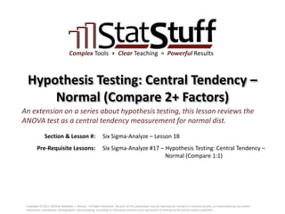
  • 1. Section & Lesson #: Pre-Requisite Lessons: Complex Tools + Clear Teaching = Powerful Results Hypothesis Testing: Central Tendency – Normal (Compare 2+ Factors) Six Sigma-Analyze – Lesson 18 An extension on a series about hypothesis testing, this lesson reviews the ANOVA test as a central tendency measurement for normal dist. Six Sigma-Analyze #17 – Hypothesis Testing: Central Tendency – Normal (Compare 1:1) Copyright © 2011-2019 by Matthew J. Hansen. All Rights Reserved. No part of this publication may be reproduced, stored in a retrieval system, or transmitted by any means (electronic, mechanical, photographic, photocopying, recording or otherwise) without prior permission in writing by the author and/or publisher.
  • 2. Why do we need hypothesis testing? o Remember, our project goal is to resolve a problem by first building a transfer function. • We don’t want to just alleviate symptoms, we want to resolve the root cause.  Remember Hannah? We don’t want to alleviate the arthritis pain in her leg, but heal the strep throat. • If we don’t know what the root cause is, then we need to build a transfer function.  By building a transfer function, we can know what changes (improvements) should fix the root cause. o Remember, the Transfer Function is defined as Y = f(X). • This is described as “output response Y is a function of one or more input X’s”. • It’s part of the IPO flow model where we described the IPO flow model as one or more inputs feeding into a process that transforms it to create a new output. o How does a transfer function fit with hypothesis testing? • Hypothesis testing tells us which X’s (inputs) are independently influencing the Y (output).  When we reject a null hypothesis, we’re building evidence proving which X’s are “guilty” of driving the Y.  We’ll compile all the evidence in the Improve phase of DMAIC and begin to fix those root causes. Copyright © 2011-2019 by Matthew J. Hansen. All Rights Reserved. No part of this publication may be reproduced, stored in a retrieval system, or transmitted by any means (electronic, mechanical, photographic, photocopying, recording or otherwise) without prior permission in writing by the author and/or publisher. Y = f(X) Input (X) > Process > Output (Y)
  • 3. Review Hypothesis Testing: 4 Step Process o Remember, the 4 high-level steps for hypothesis testing begin/end with being practical: o As the heart of hypothesis testing, steps 2 & 3 can be drilled to the following 6 steps: Copyright © 2011-2019 by Matthew J. Hansen. All Rights Reserved. No part of this publication may be reproduced, stored in a retrieval system, or transmitted by any means (electronic, mechanical, photographic, photocopying, recording or otherwise) without prior permission in writing by the author and/or publisher. 3 Practical Statistical Problem Problem Solution Solution    Practical Problem State the problem as a practical Yes/No question.  Statistical Problem Convert the problem to an analytical question identifying the statistical tool/method.  Practical Solution Interpret the analytical answer in a practical way. Statistical Solution Interpret the results of the hypothesis test with an analytical answer.  1. Define the objective. 2. State the Null Hypothesis (H0) and Alternative Hypothesis (Ha). 3. Define the confidence (1-α) and power (beta or 1-β). 4. Collect the sample data. 5. Calculate the P-value. 6. Interpret the results: accept or reject the null hypothesis (H0).
  • 4. Is the data type for both values discrete? What are you measuring? Is the data normal? SpreadCentral Tendency Compare 1:Standard 1 Proportion Test Compare 1:1 2 Proportion Test Compare 2+ Factors Chi2 Test Compare 1:Standard 1 Sample T Test Compare 1:1 2 Sample T Test or Paired T Test Compare 2+ Factors One-way ANOVA Test Compare 1:Standard 1 Sample Wilcoxon or 1 Sample Sign Compare 1:1 Mann-Whitney Test Compare 2+ Factors Mood’s Median Test or Kruskal-Wallis Test Compare 1:Standard 1 Variance Test Compare 1:1 2 Variance Test Compare 2+ Factors Test for Equal Variances Yes No Yes No Proportions Compare 1:1 Pearson Correlation or Fitted Line Plot Compare 2+ Factors Multiple Regression or General Linear Model Is the data type for both values continuous? Relationships No Yes Review Finding the Right Statistical Test o What statistical test do I use for my hypothesis testing? • The type of statistical test depends on the data to be tested, as described in the chart below: Copyright © 2011-2019 by Matthew J. Hansen. All Rights Reserved. No part of this publication may be reproduced, stored in a retrieval system, or transmitted by any means (electronic, mechanical, photographic, photocopying, recording or otherwise) without prior permission in writing by the author and/or publisher. 4 Lesson Current
  • 5. Confidence Intervals (CI) Redefined o Remember, confidence intervals (CI) are an estimated upper/lower range of the mean. • The CI narrows when you add more samples: • Remember, statistics are intended to help you make inferences about a population.  A mean of 57 with a 95% confidence interval of 55 and 59 implies that although the sample mean is only 57, you can be 95% confident that the population mean will fall somewhere between 55 and 59. • The first step in hypothesis testing is to define the objective by asking “is there a difference…”  Statistical tests generally compare the different CIs between factors to see if a difference exists. Copyright © 2011-2019 by Matthew J. Hansen. All Rights Reserved. No part of this publication may be reproduced, stored in a retrieval system, or transmitted by any means (electronic, mechanical, photographic, photocopying, recording or otherwise) without prior permission in writing by the author and/or publisher. 5 With fewer samples, the population mean falls within a wide interval. Add more samples and the population mean falls in a more narrow interval. With more samples, the more confident (narrow) the mean interval becomes. Factor A Factor B 2.5 2.75 3.0 3.25 3.5 Large overlap indicates the population mean may be the same for both groups; therefore there is no difference between them (high P-value). N = 20 Factor A Factor B 2.5 2.75 3.0 3.25 3.5 Small overlap indicates a smaller chance the population mean may be the same for both groups; therefore there is may be no difference between them (small P-value). N = 50 Factor A Factor B 2.5 2.75 3.0 3.25 3.5 No overlap indicates the population mean is different for both groups; therefore there is a difference between them (low or no P-value). N = 100
  • 6. One-Way ANOVA: Introduction o When should I use it? • To compare mean values for multiple factors. o How do I find it in Minitab? • Stat > ANOVA > One-Way… o What are the inputs for the test? Copyright © 2011-2019 by Matthew J. Hansen. All Rights Reserved. No part of this publication may be reproduced, stored in a retrieval system, or transmitted by any means (electronic, mechanical, photographic, photocopying, recording or otherwise) without prior permission in writing by the author and/or publisher. 6 Now The column containing the continuous data to test; it should represent the Y or CTQ output being measured. The factor having 2 or more discrete values that each defines the set of values for which each mean will be analyzed. Creates a visual display of 4 different charts used to analyze the residuals created by the ANOVA.
  • 7. One-Way ANOVA: Interpreting Results o How do I interpret the ANOVA results? • Below is an example of the output from an ANOVA test. • We’ll separately explore each summary and detail portion. Copyright © 2011-2019 by Matthew J. Hansen. All Rights Reserved. No part of this publication may be reproduced, stored in a retrieval system, or transmitted by any means (electronic, mechanical, photographic, photocopying, recording or otherwise) without prior permission in writing by the author and/or publisher. 7 Now Summary: This portion summarizes the results of the test. Details: This portion lists the detailed results of the test.
  • 8. One-Way ANOVA: Summary Portion o What does the summary portion of the ANOVA results mean? o What values do I use to interpret these results? • If P-value < α (0.05), statistical difference exists. • High R-sq may mean “practical” difference exists. Copyright © 2011-2019 by Matthew J. Hansen. All Rights Reserved. No part of this publication may be reproduced, stored in a retrieval system, or transmitted by any means (electronic, mechanical, photographic, photocopying, recording or otherwise) without prior permission in writing by the author and/or publisher. 8 NowSource DF SS MS F P CategoryA 4 426446 106611 2.07 0.091 Error 95 4900934 51589 Total 99 5327380 S = 227.1 R-Sq = 8.00% R-Sq(adj) = 4.13% Between analysis results Within analysis results Sources of variation Degrees of Freedom per Source (# of unique values – 1) Sum of Squares (variation) per Source Estimate of variation from each source (Calc’d as SS/DF) P valueF ratio (MSBetween )MSWithin Unexplained Variation (equals 1σ) % of variation in MetricA (Response) explained by CategoryA (Factor) (Cald’d as SSFactor / SSTotal)
  • 9. One-Way ANOVA: Detail Portion o What does the detailed portion of the ANOVA results mean? o How do I interpret these results? • Examine the difference in each unique value’s mean to see it’s significant (probably confirmed by R-sq). Copyright © 2011-2019 by Matthew J. Hansen. All Rights Reserved. No part of this publication may be reproduced, stored in a retrieval system, or transmitted by any means (electronic, mechanical, photographic, photocopying, recording or otherwise) without prior permission in writing by the author and/or publisher. 9 Now Individual 95% CIs For Mean Based on Pooled StDev Level N Mean StDev +---------+---------+---------+--------- Blue 14 524.9 182.5 (---------*---------) Green 14 362.5 141.3 (---------*---------) Red 19 559.0 226.4 (--------*-------) White 30 557.3 240.9 (-----*------) Yellow 23 539.2 270.0 (-------*-------) +---------+---------+---------+--------- 240 360 480 600 Factor’s unique values Count for each unique value Means per unique value Std Deviation per unique value Illustration of Confidence Intervals per unique value The amount of overlap in these CIs are what affect the p-value.
  • 10. One-Way ANOVA: Residuals Introduction o What are residuals? • They represent all the deviations for each data point. • Remember, a deviation is the distance a data point is from the mean. o Why are residuals used in an ANOVA test? • They help identify potential serious problems in the analysis. • It helps validate the ANOVA test to ensure the results are reliable. o What do we look for in the residuals? • Residuals should have these characteristics:  They should be normally distributed.  They should be independent.  They should have equal variances. o How do I measure the residuals? • In the ANOVA dialog box, select “Graphs…”. • In the Graphs box, select “Four in One” from the “Residual Plots” section (example at right). Copyright © 2011-2019 by Matthew J. Hansen. All Rights Reserved. No part of this publication may be reproduced, stored in a retrieval system, or transmitted by any means (electronic, mechanical, photographic, photocopying, recording or otherwise) without prior permission in writing by the author and/or publisher. 10 Now Deviation = 9 – 5 = 4 8004000-400-800 99.9 99 90 50 10 1 0.1 Residual Percent 550500450400350 500 250 0 -250 -500 Fitted Value Residual 6004002000-200-400 20 15 10 5 0 Residual Frequency 1009080706050403020101 500 250 0 -250 -500 Observation Order Residual Normal Probability Plot Versus Fits Histogram Versus Order Residual Plots for MetricA
  • 11. One-Way ANOVA: Residuals Interpretation o Interpreting the residual plots for normality: • These plotted residuals should be normally distributed. Copyright © 2011-2019 by Matthew J. Hansen. All Rights Reserved. No part of this publication may be reproduced, stored in a retrieval system, or transmitted by any means (electronic, mechanical, photographic, photocopying, recording or otherwise) without prior permission in writing by the author and/or publisher. 11 Now 8004000-400-800 99.9 99 90 50 10 1 0.1 Residual Percent 550500450400350 500 250 0 -250 -500 Fitted Value Residual 6004002000-200-400 20 15 10 5 0 Residual Frequency 1009080706050403020101 500 250 0 -250 -500 Observation Order Residual Normal Probability Plot Versus Fits Histogram Versus Order Residual Plots for MetricA 8004000-400-800 99.9 99 90 50 10 1 0.1 Residual Percent 550500450400350 500 250 0 -250 -500 Fitted Value Residual 6004002000-200-400 20 15 10 5 0 Residual Frequency 1009080706050403020101 500 250 0 -250 -500 Observation Order Residual Normal Probability Plot Versus Fits Histogram Versus Order Residual Plots for MetricA Though there’s no Anderson- Darling test, these distributions should still appear to be normal.
  • 12. One-Way ANOVA: Residuals Interpretation o Interpreting the residual plots for equal variance and independence: • These plotted residuals should appear random yet evenly spread. Copyright © 2011-2019 by Matthew J. Hansen. All Rights Reserved. No part of this publication may be reproduced, stored in a retrieval system, or transmitted by any means (electronic, mechanical, photographic, photocopying, recording or otherwise) without prior permission in writing by the author and/or publisher. 12 Now 8004000-400-800 99.9 99 90 50 10 1 0.1 Residual Percent 550500450400350 500 250 0 -250 -500 Fitted Value Residual 6004002000-200-400 20 15 10 5 0 Residual Frequency 1009080706050403020101 500 250 0 -250 -500 Observation Order Residual Normal Probability Plot Versus Fits Histogram Versus Order Residual Plots for MetricA 800 550500450400350 500 250 0 -250 -500 Fitted Value Residual 600 1009080706050403020101 500 250 0 -250 -500 Observation Order Residual Versus Fits Versus Order al Plots for MetricA The spread of plots on either side of the line should look similar. The spread of plots should look random with no patterns or trends.
  • 13. One-Way ANOVA: Boxplots o What are boxplots (a.k.a., “box and whiskers”)? • A graphical summary of a distribution’s shape, central tendency & spread. • They help compare multiple distributions and statistical characteristics. • It’s like a birds-eye view (looking down from the top) of a distribution. Copyright © 2011-2019 by Matthew J. Hansen. All Rights Reserved. No part of this publication may be reproduced, stored in a retrieval system, or transmitted by any means (electronic, mechanical, photographic, photocopying, recording or otherwise) without prior permission in writing by the author and/or publisher. 13 Now YellowWhilteRedGreenBlue 1200 1000 800 600 400 200 0 CategoryA MetricA Boxplot of MetricA **** Minitab draws each boxplot this way and lays out multiple boxplots on the same scale for easy comparison The mean is included on each boxplot with a line drawn between them. Median
  • 14. ANOVA Test: MetricA & CategoryA Example o Example: MetricA and CategoryA sample values • Background:  Use the arbitrary values in the “MetricA” and “CategoryA” columns of the Minitab Sample Data file. • Practical Problem:  Is the mean for MetricA different between the various CategoryA values? • Statistical Problem:  State the null (H0) and alternative (Ha) hypotheses: – H0: μCategoryA1 = μCategoryA2 = μCategoryA3 etc., and Ha: = μCategoryA1 ≠ μCategoryA2 ≠ μCategoryA3 etc.  Define the confidence (1-α) and power (1-β): – For confidence, we’ll accept the default of 95% (which means α = 5%) and power of 90% (which means β = 10%).  Type the statistical problem into Minitab: – In Minitab, go to Stat > ANOVA > One Way… – Select MetricA for “Response” and select CategoryA for “Factor”. – Click “Graphs…” and for “Residual Plots” select Four in one. • Statistical Solution:  Refer to the session window results. – Since P-value is > 0.05 (α), then we fail to reject H0. – R-sq(adj) suggests only 4% of variation can be explained. • Practical Solution:  The sample is insufficient to prove that the means for MetricA between each type of CategoryA value are different.  If we assumed power=90% (β=10%), then how do we apply that to this test? What does it mean? Copyright © 2011-2019 by Matthew J. Hansen. All Rights Reserved. No part of this publication may be reproduced, stored in a retrieval system, or transmitted by any means (electronic, mechanical, photographic, photocopying, recording or otherwise) without prior permission in writing by the author and/or publisher. 14 Now
  • 15. ANOVA Test: MetricA & CategoryB Example o Example: MetricA and CategoryB sample values • Background:  Use the arbitrary values in the “MetricA” and “CategoryB” columns of the Minitab Sample Data file. • Practical Problem:  Is the mean for MetricA different between the various CategoryB values? • Statistical Problem:  State the null (H0) and alternative (Ha) hypotheses: – H0: μCategoryB1 = μCategoryB2 = μCategoryB3 etc., and Ha: = μCategoryB1 ≠ μCategoryB2 ≠ μCategoryB3 etc.  Define the confidence (1-α) and power (1-β): – For confidence, we’ll accept the default of 95% (which means α = 5%) and power of 90% (which means β = 10%).  Type the statistical problem into Minitab: – In Minitab, go to Stat > ANOVA > One Way… – Select MetricA for “Response” and select CategoryB for “Factor”. – Click “Graphs…” and for “Residual Plots” select Four in one. • Statistical Solution:  Refer to the session window results. – Since P-value is > 0.05 (α), then we fail to reject H0. – R-sq(adj) suggests 0% of variation can be explained. • Practical Solution:  The sample is insufficient to prove that the means for MetricA between each type of CategoryB value are different.  If we assumed power=90% (β=10%), then how do we apply that to this test? What does it mean? Copyright © 2011-2019 by Matthew J. Hansen. All Rights Reserved. No part of this publication may be reproduced, stored in a retrieval system, or transmitted by any means (electronic, mechanical, photographic, photocopying, recording or otherwise) without prior permission in writing by the author and/or publisher. 15 Now
  • 16. Practical Application o Refer to the critical metric (output Y) and at least 5 factors (input X’s) you identified in a previous lesson for applying to this hypothesis testing. • For any factor that is a continuous value, try applying the ANOVA Test.  To do this, you’ll need a discrete factor that has 2 or more sets of values (e.g., across multiple periods of time, or different locations, or different groups, etc.).  Other factors in your organization can be used for this exercise. • Before running the ANOVA Test, do the means for each factor group appear to be different? • After running the ANOVA Test, are the means for each factor group statistically different? • If the answers to the above 2 questions are different, then how does that affect how you’d typically measure and communicate that factor in the organization?  For example, does the difference between the means affect financial decisions (e.g., how people are compensated), or process changes (e.g., how the process may be modified), or other critical actions?  If so, then how should the results from this statistical test be used to influence your organization? – Should they change how each factor group is compared (e.g., between different times, locations, groups, etc.)? – Should they change how each factor group is measured? – Should they change how they react when they compare the metric this way? Copyright © 2011-2019 by Matthew J. Hansen. All Rights Reserved. No part of this publication may be reproduced, stored in a retrieval system, or transmitted by any means (electronic, mechanical, photographic, photocopying, recording or otherwise) without prior permission in writing by the author and/or publisher. 16