Downloaded 18 times
![4
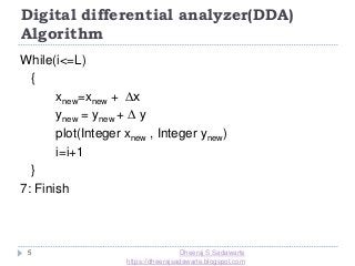
5: Initialize the initial point on the line & plot
xnew = x1 + 0.5 * (sign ∆x) &
ynew = y1 + 0.5 * (sign ∆x)
The values are rounded using the factor of 0.5
rather than truncating so that the central pixel
addressing is handled correctly.
6: [Obtain the new pixel on the line & plot the same]
Initialize i =1
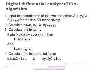
Digital differential analyzer(DDA)
Algorithm
Dheeraj S Sadawarte
https://dheerajsadawarte.blogspot.com](https://image.slidesharecdn.com/2rasterscangraphics-190804075830/85/Raster-scan-graphics-line-drawing-circle-drawing-polygon-character-generation-4-320.jpg?cb=1564905788)


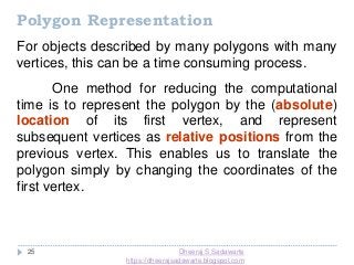

Raster scan graphics, computer graphics, line drawing algorithms, DDA line drawing, circle drawing algorithms, Bresenhams circle drawing algorithm, polygon, polygon filling, 4 connected region, 8 connected region, character generation, bitmap method, starbust method, strokes method, flood fill and boundary fill. https://dheerajsadawarte.blogspot.com/2019/08/raster-scan-graphics-computer-graphics.html