![tive radar scenarios. Even with exascale computing resources,
inversion or solution of a billion-by-billion matrix equation
will require in the order of 108
seconds, or equivalently, more
than 30 years! Hence, it is clear that raw hardware power will
not be sufficient for brute-force solutions.
III. ALGORITHMIC AND SOFTWARE SOLUTIONS
We perform exascale computations with the following build-
ing blocks:
1) Matrix-vector multiplications (MVMs) with fast multi-
pole methods (FMMs).
2) Reduced-complexity linear system solvers employing
iterative techniques.
3) Fast Fourier transforms (FFTs) with FMMs.
Fast multipole methods (FMMs) have a plethora of variations
identified with different names. For example, multilevel fast
multipole algorithm (MLFMA) [1] is an important branching
out from the single-level fast multipole algorithm. Here, we
will use FMM to refer to any and all flavors of fast multipole
algorithms (including MLFMA) developed and used in various
disciplines.
FMM can also be used to implement FFTs. This means that
FMM can be used in any discipline that requires the use of
FFT. Even better, FMM can implement FFT on nonuniform
and irregular data [2]. FFT is an important tool for feature
extraction in big-data analytics. Therefore, in addition to
extending the range of applicability of FMM among various
disciplines (through the use of FFT), we also propose a unified
approach to big-data analytics and scientific solvers with
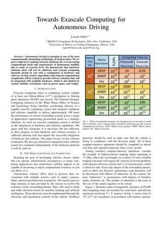
FMM. Figure 2 illustrates that employing reduced-complexity
solvers such as multilevel FMM and FFT with O(N log N)
complexity is the right way of solving extremely large prob-
lems involving billions of unknowns.
FMMs are used in a variety of disciplines, but nevertheless,
they are kernel-dependent. They can be used to acceler-
ate MVMs and linear-system solutions in many disciplines,
such as electrostatics and potential theory (Laplace’s equa-
tion), electrodynamics (Helmholtz’s equation), acoustics, as-
trophysics (gravitational force), molecular dynamics, quantum
mechanics (Schroedinger’s equation), structural mechanics,
fluid dynamics, heat equation, and multi-physics solutions.
Nevertheless, they cannot be used to perform a simple and
straightforward MVM for any arbitrary matrix and vector. It
turns out that the matrices should be constructed from specific
physical equations, whose kernels satisfy some particular
conditions, such as diagonalizability.
Fortunately, one such particular kernel that is amenable to
FMM treatment is that of the Fourier transform. Once FMM
finds life in efficient and parallel implementations of FFT,
we can penetrate into the most unimaginable capillaries of
the scientific roadmaps. Obviously, FFT is used for spectral
studies in every discipline, but its footprint is much broader
than that. FFT is used in time-harmonic treatment, complex
analysis, MVMs and matrix solutions (in some cases), and in
the vast area of big data. Not only that FMM can be used to
implement sequential and parallel FFT efficiently, but it can
also be used to compute the Fourier transform of nonuniform
and irregular multidimensional data sequences.
Parallelization of FMM is not at all trivial; on the contrary, a
scalable implementation is painstakingly difficult to attain. We
have been making progress and claiming incremental victories
in this area for more than a decade. We have been tuning our
parallelization strategies [3] so that we can achieve scalable
solutions with massive numbers of nodes, processors, and
cores on parallel supercomputers. [4] We have been solving
increasingly larger problems over the years, such as those
involving larger than billion-by-billion (109
× 109
) dense
matrix equations.
!"#$%&$'"(
)"%*+,&"%
-.$%&$'"(
)"%*+,&"%
/$+%%0$1(
-'0201$#0*1 345
6
7 89
69
89
8:
89
8;
<,='*>(
?#",$#0>" 345
;
7 89
;9
89
:
899
@01A'"BC">"'(
DEE 345
8F:
7 89
8:
8 89
B6
E+'#0BC">"'(
DEEG(DDH
345('*A(57 89
88
89
BI
89
BJ
89
89
K*2L+#01A(H02"(4%7
DC3!%
K*2L+#$#0*1$'(
K*2L'".0#=
E$#,0.(
@0M"(
457
@*'>",
Fig. 2. Order-of-magnitude estimates of computing time (in seconds) it would
take to solve matrix equations involving 10 billion unknowns via tradional and
fast solvers and with petascale and exascale computational resources.
IV. CONCLUSIONS
In this paper, we report a high-level roadmap towards sat-
isfying the ever-increasing computational needs and require-
ments of autonomous mobility. We demonstrate that hardware
solutions alone will not be sufficient, and exascale computing
demands should be met with a combination of hardware and
software. In that context, algorithms with reduced compu-
tational complexities, e.g., FMM and FFT, will be crucial
to provide software solutions that will be integrated with
available hardware, which is inherently limited due to mobility
restrictions.
REFERENCES
[1] ¨O. Erg¨ul and L. G¨urel, The Multilevel Fast Multipole Algorithm (MLFMA)
for Solving Large-Scale Computational Electromagnetics Problems.
IEEE Press-Wiley, 2014.
[2] A. Dutt and V. Rokhlin, “Fast Fourier transforms for nonequispaced data,”
SIAM J. Scientific Computing, vol. 14, no. 6, pp. 1368–1393, 1993.
[3] L. G¨urel and ¨O. Erg¨ul, “Hierarchical parallelization of the multilevel fast
multipole algorithm (MLFMA),” Proceedings of the IEEE, vol. 101, no. 2,
pp. 332–341, 2013.
[4] M. Salim, A. O. Akkirman, M. Hidayetoglu, and L. G¨urel, “Comparative
benchmarking: Matrix multiplication on a multicore coprocessor and
a GPU,” in Computational Electromagnetics International Workshop
(CEM’15), 2015, pp. 38–39.](data:image/gif;base64,R0lGODlhAQABAIAAAAAAAP///yH5BAEAAAAALAAAAAABAAEAAAIBRAA7)
Recommended
Recommended
More Related Content
What's hot
What's hot (20)
Similar to Exascale Computing for Autonomous Driving
Similar to Exascale Computing for Autonomous Driving (20)
Recently uploaded
Recently uploaded (20)
Exascale Computing for Autonomous Driving
- 1. Towards Exascale Computing for Autonomous Driving Levent G¨urel1,2 1 ABAKUS Computing Technologies, Palo Alto, California, USA 2 University of Illinois at Urbana-Champaign, Illinois, USA lgurel@illinois.edu, lgurel@ieee.org !"#$%&$'"( )"%*+,&"% -.$%&$'"( )"%*+,&"% /0! 12 13 12 2421 //! 1256 127 123 89: 1256 127 123 /0! 121; 1222 1 //! 125< 1215 127 89: 12 5< 12 15 12 7 /0! 1252 12= 122 //! 12>2 121= 1215 89: 12>2 121= 1215 12 12 ?*@A+#B9C(DB@"(E%F GHI!% /$#,B.( IA",$#B*9% /$#,B.( JBK"( ELF 12 ; 127 Fig. 1. Order-of-magnitude estimates of computing time (in seconds) it would take to perform some common matrix operations with petascale and exascale computational resources. MVP: Matrix-vector product. MMP: Matrix-matrix product. Inv: Matrix inversion. processes should be used to make sure that the vehicle is acting in compliance with the decisions made. All of those compute-intensive operations should be completed in almost real time and repeated numerous times every second. Among countless compute-intensive operations, consider the example of high-resolution imaging radars operating at 77 GHz, where the wavelength (λ) is about 3.9 mm. Credible imaging outcomes will require the solution of inverse problems with rigorous full-wave solvers and λ/10 discretization, which is about 0.4 mm. Every-day objects in the surrounding theatre, such as other cars, bicycles, pedestrians, road structures, will be discretized with billions of unknowns. In this context, the term “unknowns” is synonymous with degrees of freedom, nodes, elements, etc. The number of unknowns is the same as the size of the matrix equation to be solved. Figure 1 illustrates order-of-magnitude estimates of FLOPs and computing times (in seconds) for some basic and relevant operations involving N ×N matrices. In Fig. 1, matrix sizes of 108 –1010 are considered, in accordance with realistic automo- Abstract— Autonomous driving is emerging as one of the most computationally demanding technologies of modern times. We re- port a high-level roadmap towards satisfying the ever-increasing computational needs and requirements of autonomous mobility that is easily at exascale level. We demonstrate that hardware solutions alone will not be sufficient, and exascale computing demands should be met with a combination of hardware and software. In that context, algorithms with reduced computational complexities will be crucial to provide software solutions that will be integrated with available hardware, which is also limited by various mobility restrictions, such as power, space, and weight. I. INTRODUCTION Exascale computing refers to computing systems capable of at least one billion-billion (1018 ) calculations or floating point operations (FLOPs) per second. The National Strategic Computing Initiative of the White House Office of Science and Technology Policy identifies accelerating delivery of a capable exascale computing system that integrates hardware and software capability to deliver approximately 100 times the performance of current 10 petaflop systems across a range of applications representing government needs as a strategic objective. As such, an exascale computing system is defined as the integration of hardware and software capabilities. We agree with this viewpoint. It is necessary, but not sufficient, to drive progress in both hardware and software avenues. A sufficient outcome will also require the successful integration of hardware and software. This paper focuses on the software component. We also pay attention to integration since software cannot be considered independently of the hardware platform it will be used on. II. THE NEED FOR EXASCALE COMPUTING Reaching the goal of developing vehicles, drones, robots that can operate autonomously encompasses so many com- puting applications that autonomous mobility appears to be capable of devouring as much computational resources as you can throw at it. Autonomous vehicles (AVs) need to perceive their en- vironment with multiple sensors, such as radars, cameras, lidars, and acoustic/ultrasonic transducers. AVs need to process huge amounts of data provided by the sensors to resolve the semantics of the surrounding theater. Then, AVs need to think and make decisions based on machine learning and artificial intelligence. Those decisions must be implemented through the electronic and mechanical controls of the vehicle. Feedback
- 2. tive radar scenarios. Even with exascale computing resources, inversion or solution of a billion-by-billion matrix equation will require in the order of 108 seconds, or equivalently, more than 30 years! Hence, it is clear that raw hardware power will not be sufficient for brute-force solutions. III. ALGORITHMIC AND SOFTWARE SOLUTIONS We perform exascale computations with the following build- ing blocks: 1) Matrix-vector multiplications (MVMs) with fast multi- pole methods (FMMs). 2) Reduced-complexity linear system solvers employing iterative techniques. 3) Fast Fourier transforms (FFTs) with FMMs. Fast multipole methods (FMMs) have a plethora of variations identified with different names. For example, multilevel fast multipole algorithm (MLFMA) [1] is an important branching out from the single-level fast multipole algorithm. Here, we will use FMM to refer to any and all flavors of fast multipole algorithms (including MLFMA) developed and used in various disciplines. FMM can also be used to implement FFTs. This means that FMM can be used in any discipline that requires the use of FFT. Even better, FMM can implement FFT on nonuniform and irregular data [2]. FFT is an important tool for feature extraction in big-data analytics. Therefore, in addition to extending the range of applicability of FMM among various disciplines (through the use of FFT), we also propose a unified approach to big-data analytics and scientific solvers with FMM. Figure 2 illustrates that employing reduced-complexity solvers such as multilevel FMM and FFT with O(N log N) complexity is the right way of solving extremely large prob- lems involving billions of unknowns. FMMs are used in a variety of disciplines, but nevertheless, they are kernel-dependent. They can be used to acceler- ate MVMs and linear-system solutions in many disciplines, such as electrostatics and potential theory (Laplace’s equa- tion), electrodynamics (Helmholtz’s equation), acoustics, as- trophysics (gravitational force), molecular dynamics, quantum mechanics (Schroedinger’s equation), structural mechanics, fluid dynamics, heat equation, and multi-physics solutions. Nevertheless, they cannot be used to perform a simple and straightforward MVM for any arbitrary matrix and vector. It turns out that the matrices should be constructed from specific physical equations, whose kernels satisfy some particular conditions, such as diagonalizability. Fortunately, one such particular kernel that is amenable to FMM treatment is that of the Fourier transform. Once FMM finds life in efficient and parallel implementations of FFT, we can penetrate into the most unimaginable capillaries of the scientific roadmaps. Obviously, FFT is used for spectral studies in every discipline, but its footprint is much broader than that. FFT is used in time-harmonic treatment, complex analysis, MVMs and matrix solutions (in some cases), and in the vast area of big data. Not only that FMM can be used to implement sequential and parallel FFT efficiently, but it can also be used to compute the Fourier transform of nonuniform and irregular multidimensional data sequences. Parallelization of FMM is not at all trivial; on the contrary, a scalable implementation is painstakingly difficult to attain. We have been making progress and claiming incremental victories in this area for more than a decade. We have been tuning our parallelization strategies [3] so that we can achieve scalable solutions with massive numbers of nodes, processors, and cores on parallel supercomputers. [4] We have been solving increasingly larger problems over the years, such as those involving larger than billion-by-billion (109 × 109 ) dense matrix equations. !"#$%&$'"( )"%*+,&"% -.$%&$'"( )"%*+,&"% /$+%%0$1( -'0201$#0*1 345 6 7 89 69 89 8: 89 8; <,='*>( ?#",$#0>" 345 ; 7 89 ;9 89 : 899 @01A'"BC">"'( DEE 345 8F: 7 89 8: 8 89 B6 E+'#0BC">"'( DEEG(DDH 345('*A(57 89 88 89 BI 89 BJ 89 89 K*2L+#01A(H02"(4%7 DC3!% K*2L+#$#0*1$'( K*2L'".0#= E$#,0.( @0M"( 457 @*'>", Fig. 2. Order-of-magnitude estimates of computing time (in seconds) it would take to solve matrix equations involving 10 billion unknowns via tradional and fast solvers and with petascale and exascale computational resources. IV. CONCLUSIONS In this paper, we report a high-level roadmap towards sat- isfying the ever-increasing computational needs and require- ments of autonomous mobility. We demonstrate that hardware solutions alone will not be sufficient, and exascale computing demands should be met with a combination of hardware and software. In that context, algorithms with reduced compu- tational complexities, e.g., FMM and FFT, will be crucial to provide software solutions that will be integrated with available hardware, which is inherently limited due to mobility restrictions. REFERENCES [1] ¨O. Erg¨ul and L. G¨urel, The Multilevel Fast Multipole Algorithm (MLFMA) for Solving Large-Scale Computational Electromagnetics Problems. IEEE Press-Wiley, 2014. [2] A. Dutt and V. Rokhlin, “Fast Fourier transforms for nonequispaced data,” SIAM J. Scientific Computing, vol. 14, no. 6, pp. 1368–1393, 1993. [3] L. G¨urel and ¨O. Erg¨ul, “Hierarchical parallelization of the multilevel fast multipole algorithm (MLFMA),” Proceedings of the IEEE, vol. 101, no. 2, pp. 332–341, 2013. [4] M. Salim, A. O. Akkirman, M. Hidayetoglu, and L. G¨urel, “Comparative benchmarking: Matrix multiplication on a multicore coprocessor and a GPU,” in Computational Electromagnetics International Workshop (CEM’15), 2015, pp. 38–39.