This paper presents a novel algorithm for single image super-resolution based on gradient profile sharpness (GPS), which utilizes two gradient models to enhance edge sharpness and improve high-resolution image reconstruction. The proposed method statistically studies the GPS transformation relationship across different image resolutions, leading to better visual quality and lower reconstruction errors when compared to existing state-of-the-art techniques. Extensive experiments validate the effectiveness of the approach, demonstrating its computational efficiency and superior results in generating high-resolution images from low-resolution inputs.

1. IEEE TRANSACTIONS ON IMAGE PROCESSING, VOL. 24, NO. 10, OCTOBER 2015 3187
Single Image Superresolution Based on
Gradient Profile Sharpness
Qing Yan, Student Member, IEEE, Yi Xu, Member, IEEE, Xiaokang Yang, Senior Member, IEEE,
and Truong Q. Nguyen, Fellow, IEEE
Abstract—Single image superresolution is a classic and
active image processing problem, which aims to generate
a high-resolution (HR) image from a low-resolution input image.
Due to the severely under-determined nature of this problem, an
effective image prior is necessary to make the problem solvable,
and to improve the quality of generated images. In this paper,
a novel image superresolution algorithm is proposed based on
gradient profile sharpness (GPS). GPS is an edge sharpness
metric, which is extracted from two gradient description models,
i.e., a triangle model and a Gaussian mixture model for the
description of different kinds of gradient profiles. Then, the trans-
formation relationship of GPSs in different image resolutions
is studied statistically, and the parameter of the relationship is
estimated automatically. Based on the estimated GPS transfor-
mation relationship, two gradient profile transformation models
are proposed for two profile description models, which can keep
profile shape and profile gradient magnitude sum consistent
during profile transformation. Finally, the target gradient field of
HR image is generated from the transformed gradient profiles,
which is added as the image prior in HR image reconstruction
model. Extensive experiments are conducted to evaluate the
proposed algorithm in subjective visual effect, objective quality,
and computation time. The experimental results demonstrate that
the proposed approach can generate superior HR images with
better visual quality, lower reconstruction error, and acceptable
computation efficiency as compared with state-of-the-art
works.
Index Terms—Single image super-resolution, gradient profile
sharpness, gradient profile transformation.
I. INTRODUCTION
THE goal of single image super-resolution is to construct
a high resolution (HR) image from a low resolution (LR)
image input. This problem is an classical and active topic in
image processing, which is also a crucial step in many practical
situations, e.g. image display, remote sensing, medical imaging
and so on. However, image super-resolution problem is an
Manuscript received April 19, 2014; revised September 8, 2014 and
January 10, 2015; accepted February 14, 2015. Date of publication March 19,
2015; date of current version June 16, 2015. This work was supported
in part by the National Natural Science Foundation of China under
Grant 61025005, Grant 61201384, and Grant 61221001, in part by the
973 Program under Grant 2010CB721401, and in part by the 111 Program
under Grant B07022. The associate editor coordinating the review of this
manuscript and approving it for publication was Prof. Hitoshi Kiya.
Q. Yan, Y. Xu, and X. Yang are with the Cooperative Medianet
Innovation Center, Department of Electrical Engineering, Shanghai Jiao
Tong University, Shanghai 200030, China (e-mail: yanqing_amy@sjtu.edu.cn;
xuyi@sjtu.edu.cn; xkyang@sjtu.edu.cn).
T. Q. Nguyen is with the Department of Electrical and Computer
Engineering, University of California at San Diego, La Jolla, CA 92093 USA
(e-mail: tqn001@ucsd.edu).
Color versions of one or more of the figures in this paper are available
online at http://ieeexplore.ieee.org.
Digital Object Identifier 10.1109/TIP.2015.2414877
inherently ill-posed problem, where many HR images may
produce the same LR image when down-sampled. As a result,
how to generate an HR image with good visual perception and
as similar as its ground truth has become the goal of image
super-resolution.
There has been many research works in this field in recent
years, which can be mainly classified into three categories:
interpolation-based approaches, learning-based approaches
and reconstruction-based approaches. The interpolation-based
approaches are the basic image super-resolution methods,
where currently the bi-linear interpolation and bicubic
interpolation [1] are still very popular in practice. More
sophisticated interpolation models have also been proposed,
e.g. auto-regression model [2], multi-surface fitting model [3],
edge directed models [4], sparse representation models [5] and
ICBI (Interactive Curvature Based Interpolation) algorithm [6].
Interpolation-based approaches always have fast computation
speed. However, as pointed out in [4], interpolation-based
approaches tend to blur high frequency details if the up-scaling
ratio is large and if the low-resolution image is generated with
anti-aliasing operation.
The learning-based approaches assume that the lost high
frequency details in LR images can be retrieved and
hallucinated from a dictionary of image patch pairs. One
category of learning-based approaches learn example patches
from a data set retrieved from fixed HR image set or
website [7]–[11]. Naturally, the performance of these
approaches is highly correlated to the similarity between the
LR image patch and the learned HR image patches. To reduce
the dependence on the training HR image, self-example based
approaches were proposed, which utilized the observation that
patches tended to redundantly recur inside an image within the
same image scale as well as across different scales [12]–[15],
or there existed a transformation relationship across
image space [16]–[23]. These approaches are more robust,
however there are always some artifacts on their super-
resolution results. Generally, the computational complexity of
learning-based super-resolution approaches is quite high.
To make a tradeoff between algorithm performance and
algorithm computational efficiency, many reconstruction-based
approaches have been proposed over the years [24]–[35].
The reconstruction-based approaches enforce a constraint that
the smoothed and down-sampled version of the estimated
HR image should be consistent with its LR image. Based
on this idea, reconstruction models are proposed using
back-projection [25] or convex projection [24], [26]. To make
the ill-posed reconstruction problem solvable and to find the
1057-7149 © 2015 IEEE. Personal use is permitted, but republication/redistribution requires IEEE permission.
See http://www.ieee.org/publications_standards/publications/rights/index.html for more information.

2. 3188 IEEE TRANSACTIONS ON IMAGE PROCESSING, VOL. 24, NO. 10, OCTOBER 2015
best estimated HR image, an effective regularization term
should be added as the model constraint, which is crucial for
the reconstruction-based approaches.
Various regularization terms have been proposed based on
local gradient enhancement [27], [29]–[31] and global gradient
sparsity [32], [36]–[38]. Recently, metrics of edge sharpness
have attracted researchers attention as the regularization term,
since edges are of primary importance in visual image
quality [39]. Fattal [27] introduced the conception of gradient
profile to describe the spatial resolution of edges, where a
gradient profile is represented using three features, i.e. total
intensity change, distance from center pixel to the pixel
of zero gradient magnitude, and profile standard deviation.
Sun et.al. [29], [31] modeled the normalized gradient profile
with a GGD (generalized Gaussian distribution) model, and
adopted the standard deviation of GGD model as the edge
sharpness metric. With the help of GGD model, methods
of [29]–[31] could describe gradient profile shapes using an
adjustable and controllable model, which played an impor-
tant role in gradient profile description and transformation.
However, the GGD model is symmetric and regularly
shaped, which is hard to represent the gradient profiles with
asymmetric and complicated shapes. Furthermore, the metric
of [29]–[31] is extracted from a normalized gradient profile,
where the contrast difference between two gradient profiles
are neglected in the profile normalization step.
According to the analysis in [40], edge contrast is a key
feature for describing edge visual significance, which should
be adopted for the computation of edge sharpness. In this
paper, a novel edge sharpness metric GPS (gradient profile
sharpness) is extracted as the eccentricity of gradient profile
description models, which considers both the gradient mag-
nitude and the spatial scattering of a gradient profile.
To precisely describe different kinds of gradient profile shapes,
a triangle model and a mixed Gaussian model are proposed
for short gradient profiles and heavy-tailed gradient profiles
respectively. Then the pairs of GPS values under different
image resolutions are studied statistically, and a linear
GPS transformation relationship is formulated, whose para-
meter can be estimated automatically in each super-resolution
application. Based on the transformed GPS, two gradient
profile transformation models are proposed, which can well
keep profile shape and profile gradient magnitude sum con-
sistent during the profile transformation. Finally, the target
gradient field of HR (high resolution) image is generated
from transformed gradient profiles, which is added as the
image priors in HR image reconstruction model. Extensive
experiments are conducted to fully evaluate the proposed
super-resolution approach. It is demonstrated that the proposed
approach can generate superior HR images with better visual
similarity and lower reconstruction error as compared with
state-of-art works.
The framework of the proposed algorithm can be divided
into four parts.
• Extract GPS from two gradient profile description
models.
• Estimate GPS transformation relationship under different
image resolutions.
• Transform gradient profiles to generate the target gradient
field in HR image.
• Solve the HR reconstruction model based on estimated
target gradient field.
Corresponding to the framework, the rest of this paper is
organized as follows: The gradient profile description models
and GPS metric in the first part is defined in Section II.
Section III provides the formulation of GPS transformation
relationship and the estimation of GPS transformation para-
meter, which is applied in the second part of the framework.
The third part and the fourth part are introduced in
Section IV, where two gradient profile transformation models
are proposed and the solve of HR image reconstruction
model is introduced. Moreover, detailed experimental com-
parisons are made between the proposed approach and other
state-of-the-art super-resolution methods, which are demon-
strated in Section V. The conclusion of this work is given
in Section VI.
II. GRADIENT PROFILE DESCRIPTION MODELS
AND GPS METRIC
As initially proposed in [4], gradient profile is a feature
describing the spatial layouts of edge gradients. It is defined
as a 1D profile of gradient magnitudes along the gradient direc-
tion of an edge pixel, which is extracted by starting from an
edge pixel and tracing along the edge pixel’s gradient direction
(both sides) until the gradient magnitude does not decrease.
Generally, a sharp edge always corresponds to a group of
concentrated pixels with large gradient magnitudes, while a
smooth edge always corresponds to a group of scattered pixels
with weaker magnitudes. Hence it is possible to measure edge
sharpness using the shape of a gradient profile.
Traditional methods [29], [31] represented a gradient profile
using the GGD model, which is symmetric with a regular
shape. However, the extracted gradient profiles of most edges
are asymmetric and even with complicated shapes. In this case,
GGD model may produce large fitting errors in gradient profile
description.
To realize a better description of gradient profiles, a triangle
model and a mixed Gaussian model are proposed respectively,
where the triangle model is for gradient profiles with short
length, and the mixed Gaussian model is for gradient profiles
with heavy tails. These two models can not only accurately fit
gradient profiles with different lengths, but can also flexibly
describe gradient profiles with symmetric and asymmetric
shapes. Based on the two gradient profile description models,
GPS is defined as the eccentricity of gradient profile models.
For the convenience of profile description and profile trans-
formation, the coordinate system of each gradient profile is
normalized, where the profile peak is located at the center
x0 = 0. Then two gradient profile description models are set
up in the above-mentioned coordinate system.
A. Triangle Model
When edges are sharp or unnoticeable with small intensity
changes, the extracted gradient profiles are always short with

3. YAN et al.: SINGLE IMAGE SUPERRESOLUTION BASED ON GPS 3189
Fig. 1. The fitting results of triangle model and GGD model for short gradient
profiles. (a) Fitting results of symmetric gradient profiles. (b) Fitting results of
asymmetric gradient profiles. The blue starts are the extracted profile points,
the red lines are the fitting results of triangle model, and the green curves are
the fitting results of GGD model.
no tails. For this kind of gradient profiles, a triangle model is
most suitable for the profile description.
To flexibly represent a gradient profile, the two sides of the
triangle model are fitted separately using the extracted gradient
profile points of each side. The linear function of each profile
side is formulated as
mT (x) =
kdx + h, if the value ≥ 0
0 otherwise
(1)
where mT (x) is the gradient magnitude of pixel x in the
triangle model, dx is the distance between the pixel x and
the profile peak x0, k and h are the slope-intercept parameters
of the linear function. The peak value of the triangle model
is constrained to be the maximum magnitude of provided
gradient profile, which is denoted as h in (1).
The slope k is fitted using the pixels on the corresponding
side of provided gradient profile,
k = min
k
x∈p
[m(x) − k · dx − h]2
, (2)
where m(x) is the gradient magnitude of pixel x on the
provided gradient profile p.
Four fitting examples of short gradient profiles are shown
in Fig. 1, where the blue stars are the extracted gradient profile
points and the red lines are the fitting results of proposed
triangle model. To make a comparison, the fitting results
of GGD model [31] (the green curves) are also provided.
As shown in Fig. 1(a), it is hard to estimate an accurate
GGD model with only a small number of extracted gradient
profile points, so there is large fitting error at the gradient
profile peak. Moreover, when gradient profiles are asymmetric
as shown in Fig. 1(b), the fitting error of GGD model is even
larger. Compared with GGD model, the triangle model is quite
flexible, which can well represent gradient profiles with both
symmetric and asymmetric shapes.
Fig. 2. The histogram of profile length under different up-scaling ratios
(R=2, 3, 4).
B. Mixed Gaussian Model
When edges are smooth, gradient profiles become longer
and profile shapes become complicated with heavy tails.
For such kind of gradient profiles, a mixed Gaussian
model is proposed, which is a mixture of two Gaussian
models
mG(x)
=
⎧
⎪⎨
⎪⎩
a1
√
2πb1
e
−(x−c1)2
2b2
1 +
a2
√
2πb2
e
−(x−c2)2
2b2
2 if the value ≥ 0
0 otherwise.
(3)
The parameters of a1 and a2 are the mixing rates of each
Gaussian model, which can be two positive numbers or a
positive value and a negative one. The parameters of b1 and b2
are the standard deviations and c1 and c2 are the mean values
of two Gaussian models.
The six parameters are estimated using the ‘lsqcurvefit’
function in Matlab. To ensure the mixed Gaussian model is
unimodal, a regularization term about c1 and c2 is added in
the parameter estimation process,
(a∗
1, b∗
1, c∗
1, a∗
2, b∗
2, c∗
2)
= min
(a1,b1,c1,a2,b2,c2)
×
x∈p
m(x) −
a1
√
2πb1
e
−(x−c1)2
2b2
1 −
a2
√
2πb2
e
−(x−c2)2
2b2
2
2
+ β(c1 − c2)2
(4)
where β is the regularization coefficient, which is empirically
set to be 0.1.
According to (3), there are six parameters in the mixed
Gaussian model, so there should be at least six extracted gradi-
ent profile points input in (4). To realize a robust and accurate
parameter estimation, the number of input profile points should
be as large as possible. However, according to the distribution
histograms of gradient profile length, which is shown in Fig. 2,
the histogram of profile length decreases dramatically as the
profile length increases. (Each histogram is generated using

4. 3190 IEEE TRANSACTIONS ON IMAGE PROCESSING, VOL. 24, NO. 10, OCTOBER 2015
Fig. 3. The fitting results of mixed Gaussian model and GGD model for long
gradient profiles. (a) Fitting results of gradient profiles with regular shapes.
(b) Fitting results of gradient profiles with complicated shapes. The blue starts
are the extracted profile points, the red curves are the fitting results of mixed
Gaussian model, and the green curves are the fitting results of GGD model.
the 29,000 randomly extracted gradient profiles in the
up-sampled reference images of LIVE database [41].) Thus,
fewer gradient profiles can be described by mixed Gaussian
model when there is a large threshold set on gradient profile
length. To make a balance, it is assumed that only the gradient
profiles with more than eight profile points are described by
the mixed Gaussian model.
Eight fitting examples of heavy-tailed gradient profiles are
provided in Fig. 3, where the first four gradient profiles
are nearly symmetric with regular shapes and the other four
gradient profiles are asymmetric with complicated shapes. It is
shown both two models can produce good fitting results when
profiles are symmetric. However, when gradient profiles are
symmetric, the proposed mixed Gaussian model has much
better performance than the GGD model, which is more
flexible to describe the detail shape changes in the gradient
profiles with complicated shapes.
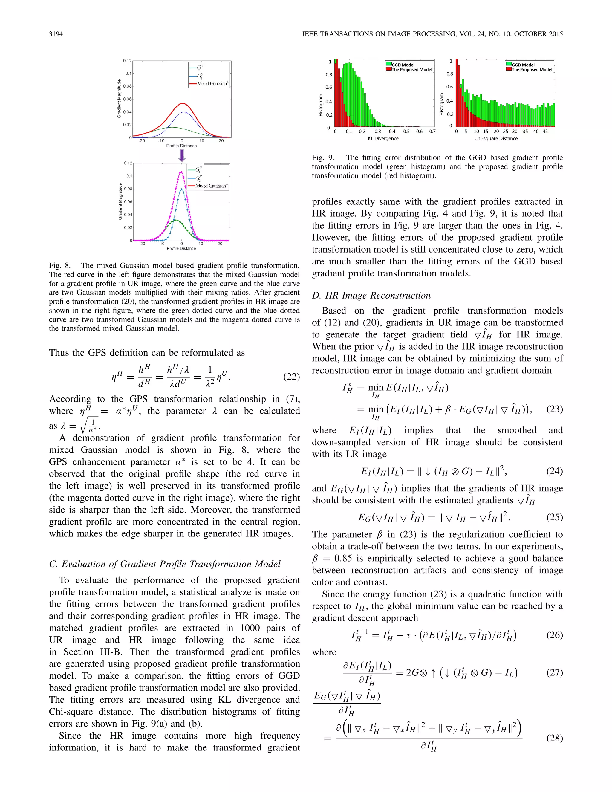
C. Evaluation of Gradient Profile Fitting Performance
To evaluate the fitting performance of proposed gradient
profile description models, an image set containing
1000 images from the INRIAPerson dataset [42] is adopted
for gradient profile extraction. For each image, edges are
detected using Canny algorithm [43]. Then, 1000 edge pixels
Fig. 4. The fitting error distributions of the GGD model and the proposed
model.
are selected randomly to produce 1000 gradient profiles. For
each gradient profile, both the GGD model and the proposed
gradient profile description models are adopted in the fitting
process.
For each gradient profile, if there are less than 8 extracted
profile points, the triangle model is applied; Otherwise, both
the mixed Gaussian model and the triangle model are applied,
and only the one with smaller fitting error is adopted in the
gradient profile description. In this way, the wrongly estimated
mixed Gaussian models can be well removed.
The fitting errors of GGD model and the proposed models
are measured using Kullback-Leibler (KL) divergence and
Chi-square distance. The distributions of fitting error are
shown in Fig. 4, where the green histogram belongs to the
GGD model and the red histogram belongs to the proposed
models. It is observed that the fitting errors of the proposed
models are dominantly distributed close to zero whether they
are measured by KL divergence or Chi-square distance. The
fitting errors of GGD model are concentrated at 0.06 using
KL divergence and concentrated at 12 using Chi-square
distance.
Based on the statistical evaluation on gradient profile fitting
error, the proposed models are more appropriate for gradient
profile description. Such precise gradient profile description
models will contribute a lot for preserving the illumination
change details around edge pixels.
D. GPS Definition
The key features of the triangle model and the mixed
Gausssian model are their height h and spatial scattering d.
Thus a metric of gradient profile sharpness (GPS) is defined
based on the eccentricity of two gradient profile description
models, which is the ratio of the height to the spatial scattering
η = h/d. (5)
The height h represents the edge contrast of extracted
gradient profile, which is the maximum gradient magnitude
of the gradient profile. The spatial scattering d represents
the edge spatial spread of extracted gradient profile. For
triangle model, it is defined as the distance between the
horizontal intersection points when the mT (x) in (1) equals
zero. For mixed Gaussian model, it is the distance between the
two points that mG(x) stops decreasing, which is the points
whose averaged decrease value is smaller than 5%·h (or 0.001
when h is very small), |mG (x−1)−mG(x)|+|mG(x)−mG(x+1)|
2 <
max(0.05 · h, 0.001). (The range of gradient magnitude is
normalized to [0, 1].)

5. YAN et al.: SINGLE IMAGE SUPERRESOLUTION BASED ON GPS 3191
Fig. 5. Edge sharpness representation using GPS. (a) The original image.
(b) The edge sharpness image obtained using GPS. The GPS values are
normalized to [0, 1], where a larger value implies a sharper edge. The
corresponding color of each GPS value is demonstrated by the color bar.
GPS takes both edge contrast and edge spatial scattering in
its consideration. Since edge contrast plays an important role
in human perception of edge sharpness, GPS can represent
edge sharpness perceptually well. Two examples are shown
in Fig. 5, where the GPS values are normalized to [0, 1].
A larger GPS value implies a sharper edge, and the
corresponding color for each GPS value is demonstrated by
the color bar on the right. As shown in Fig. 5(a), there are
both sharp edges (in the regions of parrot and flower) and
smooth edges (in the background which is out-of-focus) in
the original images. The GPS results are shown in Fig. 5(b),
where sharp edges and smooth edges can be distinguished
easily. The smooth edges in the background always have the
smallest GPS values, while the sharp edges in the regions of
Parrots eyes and flower always have large GPS values, which
is consistent with human perception. Thus GPS is robust and
appropriate for edge sharpness description.
III. ESTIMATE GPS TRANSFORMATION RELATIONSHIP
To obtain the target gradient field for HR image reconstruc-
tion, the gradient profiles in LR image should be transformed
into the ones in HR image. To formulate gradient profile
transformation model, the relationship of GPSs in different
image resolutions should be studied, and the parameter in the
GPS relationship should be well estimated.
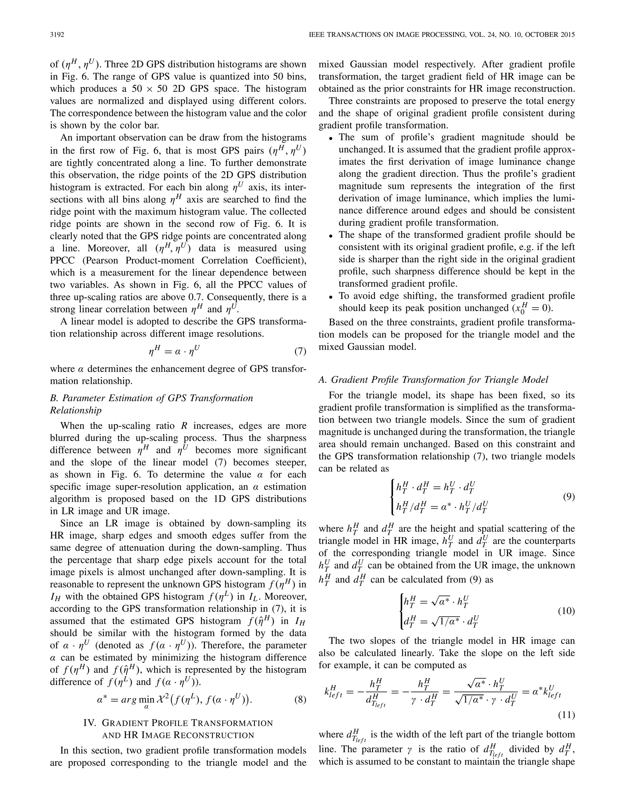
A. The Study of GPS Transformation Relationship
Following the previous works of [27], [31], and [44],
the relationship of GPSs in HR images and LR images is
represented using the relationship of GPSs in HR images and
up-scaled images (denoted as UR image). Thus a group of
corresponding GPS pairs (ηH , ηU ) are collected.
Given an HR image IH , its LR image IL is generated by
down-sampling IH according to the down-sampling ratio 1/R.
Then an UR image IU is obtained by interpolating IL accord-
ing to the up-scaling ratio R, which produces an image
pair of (IH , IU ). After that, edge pixels in IU are detected
using Canny algorithm [43]. For each edge pixel xU
0 in IU,
Fig. 6. The study of GPS transformation relationship. The first row
contains three 2D GPS distribution histograms, where the histogram values
are normalized to [0, 1] and displayed using different colors. The
corresponding color for each histogram value is demonstrated by the color
bar on the right side. The second row contains the ridge points of the
2D GPS distribution histogram. The third row includes the PPCC (Pearson
Product-moment Correlation Coefficient) coefficients of the GPS data in the
first row. (a), (b) and (c) are the corresponding results under three up-sale
ratios R = 2, 3, 4.
its corresponding edge pixel in IH is searched by comparing
pixel spatial distance and pixel gradient difference,
x H
0 = arg min
x∈N
d(x, xU
0 )2
+ β ·
−→
GH (x) −
−→
GU (xU
0 ) 2
(6)
where d(x, xU
0 ) is the spatial distance between the positions
of x and xU
0 , and
−→
GH (x)−
−→
GU (xU
0 ) is the magnitude of the
gradient difference between gradient vectors of x and xU
0 .
The gradient vector contains the gradients in horizontal and
vertical directions, where the magnitude range of gradient
vector is normalized to [0, 1]. The maximum magnitude of
gradient difference vector is 2, which can be obtained when
−→
GH (x) =
1
0
, and
−→
GU (xU
0 ) =
−1
0
. Thus the range of
−→
G H (x) −
−→
G U (xU
0 ) 2 in (6) is [0, 4].
The N in (6) is the neighborhood region centered
at xU
0 ’s position in IH , which is set to be 5 × 5 in this paper.
Thus the largest distance value of d(x, xU
0 ) is 2
√
2, and the
range of d(x, xU
0 )2 is [0, 8].
To make a balance between the two terms in (6), the
regularization coefficient β is set to be 2. When the
corresponding edge pixels (x H
0 , xU
0 ) are obtained, a pair of
corresponding gradient profiles are extracted from IH and IU
at the positions of x H
0 and xU
0 , then the GPS pair (η(x H
0 ),
η(xU
0 )) is calculated according to (5).
The GPS relationship is studied under three up-scaling
ratios R = 2, 3, 4. The image set of 1000 photos from
INRIAPerson dataset [42] is adopted to produce I H images.
The corresponding IU is generated by down-sampling from
I H and then interpolated back. At each up-scaling ratio,
1000 pairs of (x H
0 , xU
0 ) are collected randomly from each
pair of IH and IU, which produces 1,000,000 GPS pairs of
(η(x H
0 ), η(xU
0 )) in total.
Based on these GPS pairs, GPS relationship can be
demonstrated using the distribution histogram in 2D space

6. 3192 IEEE TRANSACTIONS ON IMAGE PROCESSING, VOL. 24, NO. 10, OCTOBER 2015
of (ηH , ηU ). Three 2D GPS distribution histograms are shown
in Fig. 6. The range of GPS value is quantized into 50 bins,
which produces a 50 × 50 2D GPS space. The histogram
values are normalized and displayed using different colors.
The correspondence between the histogram value and the color
is shown by the color bar.
An important observation can be draw from the histograms
in the first row of Fig. 6, that is most GPS pairs (ηH, ηU )
are tightly concentrated along a line. To further demonstrate
this observation, the ridge points of the 2D GPS distribution
histogram is extracted. For each bin along ηU axis, its inter-
sections with all bins along ηH axis are searched to find the
ridge point with the maximum histogram value. The collected
ridge points are shown in the second row of Fig. 6. It is
clearly noted that the GPS ridge points are concentrated along
a line. Moreover, all (ηH, ηU ) data is measured using
PPCC (Pearson Product-moment Correlation Coefficient),
which is a measurement for the linear dependence between
two variables. As shown in Fig. 6, all the PPCC values of
three up-scaling ratios are above 0.7. Consequently, there is a
strong linear correlation between ηH and ηU.
A linear model is adopted to describe the GPS transforma-
tion relationship across different image resolutions.
ηH
= α · ηU
(7)
where α determines the enhancement degree of GPS transfor-
mation relationship.
B. Parameter Estimation of GPS Transformation
Relationship
When the up-scaling ratio R increases, edges are more
blurred during the up-scaling process. Thus the sharpness
difference between ηH and ηU becomes more significant
and the slope of the linear model (7) becomes steeper,
as shown in Fig. 6. To determine the value α for each
specific image super-resolution application, an α estimation
algorithm is proposed based on the 1D GPS distributions
in LR image and UR image.
Since an LR image is obtained by down-sampling its
HR image, sharp edges and smooth edges suffer from the
same degree of attenuation during the down-sampling. Thus
the percentage that sharp edge pixels account for the total
image pixels is almost unchanged after down-sampling. It is
reasonable to represent the unknown GPS histogram f (ηH ) in
IH with the obtained GPS histogram f (ηL) in IL. Moreover,
according to the GPS transformation relationship in (7), it is
assumed that the estimated GPS histogram f (ˆηH ) in IH
should be similar with the histogram formed by the data
of α · ηU (denoted as f (α · ηU )). Therefore, the parameter
α can be estimated by minimizing the histogram difference
of f (ηH ) and f (ˆηH ), which is represented by the histogram
difference of f (ηL) and f (α · ηU )).
α∗
= arg min
α
X2
f (ηL
), f (α · ηU
) . (8)
IV. GRADIENT PROFILE TRANSFORMATION
AND HR IMAGE RECONSTRUCTION
In this section, two gradient profile transformation models
are proposed corresponding to the triangle model and the
mixed Gaussian model respectively. After gradient profile
transformation, the target gradient field of HR image can be
obtained as the prior constraints for HR image reconstruction.
Three constraints are proposed to preserve the total energy
and the shape of original gradient profile consistent during
gradient profile transformation.
• The sum of profile’s gradient magnitude should be
unchanged. It is assumed that the gradient profile approx-
imates the first derivation of image luminance change
along the gradient direction. Thus the profile’s gradient
magnitude sum represents the integration of the first
derivation of image luminance, which implies the lumi-
nance difference around edges and should be consistent
during gradient profile transformation.
• The shape of the transformed gradient profile should be
consistent with its original gradient profile, e.g. if the left
side is sharper than the right side in the original gradient
profile, such sharpness difference should be kept in the
transformed gradient profile.
• To avoid edge shifting, the transformed gradient profile
should keep its peak position unchanged (x H
0 = 0).
Based on the three constraints, gradient profile transforma-
tion models can be proposed for the triangle model and the
mixed Gaussian model.
A. Gradient Profile Transformation for Triangle Model
For the triangle model, its shape has been fixed, so its
gradient profile transformation is simplified as the transforma-
tion between two triangle models. Since the sum of gradient
magnitude is unchanged during the transformation, the triangle
area should remain unchanged. Based on this constraint and
the GPS transformation relationship (7), two triangle models
can be related as
⎧
⎨
⎩
hH
T · dH
T = hU
T · dU
T
hH
T /dH
T = α∗ · hU
T /dU
T
(9)
where hH
T and dH
T are the height and spatial scattering of the
triangle model in HR image, hU
T and dU
T are the counterparts
of the corresponding triangle model in UR image. Since
hU
T and dU
T can be obtained from the UR image, the unknown
hH
T and dH
T can be calculated from (9) as
⎧
⎨
⎩
hH
T =
√
α∗ · hU
T
dH
T =
√
1/α∗ · dU
T
(10)
The two slopes of the triangle model in HR image can
also be calculated linearly. Take the slope on the left side
for example, it can be computed as
kH
lef t = −
hH
T
dH
Tlef t
= −
hH
T
γ · dH
T
=
√
α∗ · hU
T
√
1/α∗ · γ · dU
T
= α∗
kU
lef t
(11)
where dH
Tlef t
is the width of the left part of the triangle bottom
line. The parameter γ is the ratio of dH
Tlef t
divided by dH
T ,
which is assumed to be constant to maintain the triangle shape

7. YAN et al.: SINGLE IMAGE SUPERRESOLUTION BASED ON GPS 3193
Fig. 7. The transformation of two triangle models, where the triangle area
and shape remain unchanged during the transformation.
during the transformation. The same procedure can also be
imposed on the calculation of dH
Tright
.
The gradient magnitude of each point on the gradient
profile can be transformed linearly. For example, the gradient
magnitude of pixel xi on the left side of the gradient profile
can be calculated as
ˆmH
x =
kH
lef t dx + hH
T if dx ≤ dH
Tlef t
0 otherwise
(12)
where dx is the distance between xi and the edge pixel x0.
The whole gradient profile transformation of triangle model is
demonstrated in Fig. 8.
B. Gradient Profile Transformation for
Mixed Gaussian Model
For mixed Gaussian model, its shape is not as regular as the
triangle model, thus its transformation is more complicated.
Suppose the spatial range of original gradient profile is
within [dU
Glef t
, dU
Gright
], the spatial range of transformed
gradient profile is with [dH
Glef t
, dH
Gright
], and the spatial scat-
tering dH
G is reduced by a ratio of λ during the transformation
(dH
G = λdU
G ). To keep profile shape consistent during the
gradient profile transformation, the ratio of dH
Glef t
to dH
G
should be equal to the ratio of dU
Glef t
to dU
G , which implies
that
dH
Glef t
= λdU
Gle f t
and dH
Gright
= λdU
Gright
. (13)
Since the gradient magnitude sum in mixed Gaussian model
is unchanged during the transformation, then
dU
Gright
dU
Glef t
aU
1
√
2πbU
1
e
−(x−cU
1 )2
2(bU
1 )2
+
aU
2
√
2πbU
2
e
−(x−cU
2 )2
2(bU
2 )2
dx
=
dH
Gright
dH
Glef t
aH
1
√
2πbH
1
e
−(x−cH
1 )2
2(bH
1 )2
+
aH
2
√
2πbH
2
e
−(x−cH
2 )2
2(bH
2 )2
dx.
(14)
To satisfy (14) and keep the shape of mixed Gaussian model
consistent, each Gaussian model is assumed to preserve its
gradient magnitude sum respectively.
⎧
⎪⎪⎪⎪⎪⎨
⎪⎪⎪⎪⎪⎩
dU
Gright
dU
Gle f t
aU
1
√
2πbU
1
e
−(x−cU
1 )2
2(bU
1 )2
dx =
dH
Gright
dH
Glef t
aH
1
√
2πbH
1
e
−(x−cH
1 )2
2(bH
1 )2
dx
dU
Gright
dU
Glef t
aU
2
√
2πbU
2
e
−(x−cU
2 )2
2(bU
2 )2
dx =
dH
Gright
dH
Glef t
aH
2
√
2πbH
2
e
−(x−cH
2 )2
2(bH
2 )2
dx
(15)
Based on the scattering range equation (13), the right part of
the first equation in (15) can be reformulated as
dH
Gright
dH
Gle f t
aH
1
√
2πbH
1
e
−(x−cH
1 )2
2(bH
1 )2
dx =
λdU
Gright
λdU
Glef t
aH
1
√
2πbH
1
e
−(x−cH
1 )2
2(bH
1 )2
dx.
(16)
Denote x = λz, (16) can be reformulated as
λdU
Gright
λdU
Glef t
aH
1
√
2πbH
1
e
−(x−cH
1 )2
2(bH
1 )2
dx
=
dU
Gright
dU
Glef t
λaH
1
√
2πbH
1
e
−(λz−cH
1 )2
2(bH
1 )2
dz
=
dU
Gright
dU
Glef t
aH
1
√
2π
bH
1
λ
e
−(z−
cH
1
λ )2
2(
bH
1
λ )2
dz. (17)
Thus the equations of (15) can be expressed as
⎧
⎪⎪⎪⎪⎪⎪⎪⎪⎪⎨
⎪⎪⎪⎪⎪⎪⎪⎪⎪⎩
dU
Gright
dU
Glef t
aU
1
√
2πbU
1
e
−(x−cU
1 )2
2(bU
1 )2
dx =
dU
Gright
dU
Gle f t
aH
1
√
2π
bH
1
λ
e
−(z−
cH
1
λ )2
2(
bH
1
λ )2
dz
dU
Gright
dU
Glef t
aU
2
√
2πbU
2
e
−(x−cU
2 )2
2(bU
2 )2
dx =
dU
Gright
dU
Gle f t
aH
2
√
2π
bH
2
λ
e
−(z−
cH
2
λ )2
2(
bH
2
λ )2
dz.
(18)
Based on (18), the relationship between the Gaussian
parameters are as follows
⎧
⎨
⎩
aH
1 = aU
1 , bH
1 = λbU
1 , cH
1 = λcU
1
aH
2 = aU
2 , bH
2 = λbU
2 , cH
2 = λcU
2 .
(19)
Thus the mixed Gaussian model for HR image is
mG(x)
=
⎧
⎪⎨
⎪⎩
aU
1
√
2πλbU
1
e
−(x−λcU
1 )2
2(λbU
1 )2
+
aU
2
√
2πλbU
2
e
−(x−λcU
2 )2
2(λbU
2 )2
if the value ≥ 0
0 otherwise
(20)
There is only one parameter λ to be estimated in the
gradient profile transformation model of mixed Gaussian
model. According to the GPS definition, there is
ηH = hH /dH , where dH = λdU and hH can be approximated
by the peak value of mG(0) in (20).
hH
=
aU
1
√
2πλbU
1
e
−(λcU
1 )2
2(λbU
1 )2
+
aU
2
√
2πλbU
2
e
−(λcU
2 )2
2(λbU
2 )2
=
1
λ
·
aU
1
√
2πbU
1
e
−(cU
1 )2
2(bU
1 )2
+
aU
2
√
2πbU
2
e
−(cU
2 )2
2(bU
2 )2
=
hU
λ
. (21)

8. 3194 IEEE TRANSACTIONS ON IMAGE PROCESSING, VOL. 24, NO. 10, OCTOBER 2015
Fig. 8. The mixed Gaussian model based gradient profile transformation.
The red curve in the left figure demonstrates that the mixed Gaussian model
for a gradient profile in UR image, where the green curve and the blue curve
are two Gaussian models multiplied with their mixing ratios. After gradient
profile transformation (20), the transformed gradient profiles in HR image are
shown in the right figure, where the green dotted curve and the blue dotted
curve are two transformed Gaussian models and the magenta dotted curve is
the transformed mixed Gaussian model.
Thus the GPS definition can be reformulated as
ηH
=
hH
dH
=
hU /λ
λdU
=
1
λ2
ηU
. (22)
According to the GPS transformation relationship in (7),
where ηH = α∗ηU , the parameter λ can be calculated
as λ = 1
α∗ .
A demonstration of gradient profile transformation for
mixed Gaussian model is shown in Fig. 8, where the
GPS enhancement parameter α∗ is set to be 4. It can be
observed that the original profile shape (the red curve in
the left image) is well preserved in its transformed profile
(the magenta dotted curve in the right image), where the right
side is sharper than the left side. Moreover, the transformed
gradient profile are more concentrated in the central region,
which makes the edge sharper in the generated HR images.
C. Evaluation of Gradient Profile Transformation Model
To evaluate the performance of the proposed gradient
profile transformation model, a statistical analyze is made on
the fitting errors between the transformed gradient profiles
and their corresponding gradient profiles in HR image. The
matched gradient profiles are extracted in 1000 pairs of
UR image and HR image following the same idea
in Section III-B. Then the transformed gradient profiles
are generated using proposed gradient profile transformation
model. To make a comparison, the fitting errors of GGD
based gradient profile transformation model are also provided.
The fitting errors are measured using KL divergence and
Chi-square distance. The distribution histograms of fitting
errors are shown in Fig. 9(a) and (b).
Since the HR image contains more high frequency
information, it is hard to make the transformed gradient
Fig. 9. The fitting error distribution of the GGD based gradient profile
transformation model (green histogram) and the proposed gradient profile
transformation model (red histogram).
profiles exactly same with the gradient profiles extracted in
HR image. By comparing Fig. 4 and Fig. 9, it is noted that
the fitting errors in Fig. 9 are larger than the ones in Fig. 4.
However, the fitting errors of the proposed gradient profile
transformation model is still concentrated close to zero, which
are much smaller than the fitting errors of the GGD based
gradient profile transformation models.
D. HR Image Reconstruction
Based on the gradient profile transformation models
of (12) and (20), gradients in UR image can be transformed
to generate the target gradient field ˆIH for HR image.
When the prior ˆIH is added in the HR image reconstruction
model, HR image can be obtained by minimizing the sum of
reconstruction error in image domain and gradient domain
I∗
H = min
IH
E(IH |IL, ˆIH )
= min
IH
EI (IH |IL) + β · EG( IH | ˆIH ) , (23)
where EI (IH |IL) implies that the smoothed and
down-sampled version of HR image should be consistent
with its LR image
EI (IH |IL) = ↓ (IH ⊗ G) − IL
2
, (24)
and EG( IH | ˆIH ) implies that the gradients of HR image
should be consistent with the estimated gradients ˆIH
EG( IH | ˆIH ) = IH − ˆIH
2
. (25)
The parameter β in (23) is the regularization coefficient to
obtain a trade-off between the two terms. In our experiments,
β = 0.85 is empirically selected to achieve a good balance
between reconstruction artifacts and consistency of image
color and contrast.
Since the energy function (23) is a quadratic function with
respect to IH , the global minimum value can be reached by a
gradient descent approach
It+1
H = It
H − τ · ∂ E(It
H |IL, ˆIH )/∂ It
H (26)
where
∂ EI (It
H |IL)
∂ It
H
= 2G⊗ ↑ ↓ (It
H ⊗ G) − IL (27)
EG( It
H | ˆIH )
∂ It
H
=
∂ x It
H − x ˆIH
2 + y It
H − y ˆIH
2
∂ It
H
(28)

9. YAN et al.: SINGLE IMAGE SUPERRESOLUTION BASED ON GPS 3195
Denote x It
H = It
H Dx , y It
H = Dy It
H , equation (28)
becomes
EG( It
H | ˆIH )
∂ It
H
= 2 It
H Dx DT
x − x ˆIH DT
x + DT
y Dy It
H − DT
y y ˆIH (29)
In the implementation of (26), the step size τ is set to be 0.2,
the up-scaled image IU is used as the initial value of IH , and
the iteration number is set to be 100. These parameters are
not sensitive to different super-resolution applications.
V. EXPERIMENTAL RESULTS
To fully evaluate the proposed approach, comparisons
between the proposed approach and the state-of-the-art super-
resolution approaches are made on subjective visual effect,
objective quality, and computation time. Given a colorful
LR image, the image is first transformed from RGB color
space to YUV color space, and super-resolution is performed
only on the luminance channel image. In this way, there is
less color distortions in the estimated HR image. The test
LR images in Section V-A and V-B can be downloaded
from public web sites [45]–[47], and the test LR image
in Section V-C are generated by directly down-sampling from
their corresponding HR images.
As mentioned above, the enhancement parameter α in (7)
is learned according to (8), the weight β in (23) is set to
be 0.85, and the step size τ in (26) is set to be 0.2. The
Gaussian kernel G in (24) has different sizes according to
different up-scaling factors: a 3 × 3 mask with a standard
deviation of 0.8 for X2 super-resolution, a 5 × 5 mask with a
standard deviation of 1.2 for X3 super-resolution, a 7×7 mask
with standard deviation of 1.4 for X4 super-resolution, and
a 9 × 9 with standard deviation of 1.6 for the super-resolution
reconstruction whose up-scaling factor is larger than 4.
Since the approach Sun11 in [31] and the proposed approach
both solve the image super-resolution problem by modeling
edge gradient profiles, the two approaches are compared
first. Then the proposed method is compared with other
interpolation-based, learning-based and reconstruction-based
image super-resolution approaches.
A. Comparison With Gradient Profile Based
Super-Resolution Method
The main difference between the work Sun11 [31] and the
proposed approach are in four aspects, which are listed as
below:
1) The work Sun11 [31] adopted symmetric GGD model
for its gradient profile description. The proposed
approach utilizes triangle model and mixed Gaussian
model to describe gradient profiles with different lengths
and complicated asymmetric shapes, which are more
flexible to produce better fitting performance.
2) The edge sharpness metric of Sun11 [31] is based on
normalized gradient profile, where the magnitude dif-
ference between different gradient profiles is neglected
during profile normalization. The proposed metric GPS
considers both gradient profile’s gradient magnitude
Fig. 10. The comparison between the method in [31] and the proposed
method. The up-scaling ratio of image Head is 4 (LR is 70 × 70
and HR is 280 × 280), and the up-scaling ratio of Lady and Starfish
is 3 (LR is 107 × 160 and HR is 321 × 480).
and spatial scattering, which emphasizes the impact of
illumination contrast on human visual perception.
3) The work Sun11 [31] proposed an exponential sharpness
enhancement function. The proposed approach has a
linear GPS transformation relationship between differ-
ent image resolutions, where its validity is proved by
the PPCC values in Fig. 6. Moreover, the parame-
ter of GPS transformation model can be estimated
automatically for each specific image super-resolution
application.
4) In the work Sun11 [31], gradient profiles are transformed
to be symmetric due to the symmetric GGD model.
In the proposed approach, gradient profiles are trans-
formed under the constraint that the sum of gradient
magnitude and the shape of gradient profile should be
consistent during the transformation. Based on these
constraint, gradient profiles are enhanced according
to their original shapes, which makes the generated
HR image more close to the ground truth.
Three super-resolution comparisons between the
method Sun11 [31] and the proposed approach are provided
in Fig. 10. The three images are the publicly available
images that Sun11 [31] had provided their ground truth

10. 3196 IEEE TRANSACTIONS ON IMAGE PROCESSING, VOL. 24, NO. 10, OCTOBER 2015
Fig. 11. The 4X super-resolution on ‘Baby’ image. LR is 128 × 128, and HR is 512 × 512. (a) Freeman02 [7]. (b) Glasner09 [13]. (c) Freedman11 [14].
(d) BPJDL13 [17]. (e) ICBI11 [6]. (f) Fattal07 [27]. (g) Shan08 [32]. (h) Our result.
HR images, estimated HR images and objective measurement
results totally. The objective measurements adopted in
the comparison are RMS (Root Mean Square) and SSIM
(Structural SIMilarity) [48], where RMS is a measurement
for reconstruction error and SSIM is a measurement for the
structural similarity between the estimated HR image and the
ground truth HR image. A lower RMS value and a higher
SSIM value represent a better reconstruction result.
As demonstrated by the results in Fig. 10, the proposed
approach outperforms the method Sun11 [31] in both
objective and subjective measures. The proposed approach
can generate clearer HR images with little artifacts, since
GPS is more consistent with human perception and the
proposed gradient profile description models are more
accurate. The objective measurements also show that the
HR image estimated by the proposed approach is more
consistent with the ground truth HR image in higher visual
similarity and lower reconstruction error.
B. More Comparisons With the State-of-the-Art Methods
The proposed method is compared with more
state-of-the-art super-resolution methods, which include
one interpolation-based method (ICBI11 [6]), three
reconstruction-based methods (Fattal07 [27], Shan08 [32] and
Sun11 [31]), four learning-based methods (Freeman02 [7],
Glasner09 [13] and Freedman11 [14], BPJDL13 [17]), and
one leading commercial product Genuine FractalsTM [49].
The super-resolution results of [6], [7], [13], [14], [27], [31],
and [32] are available from the public website of [45]–[47].
The comparison results are shown in Fig. 11 to Fig. 13.
In general, it can be observed that the interpolation-based
method [6] and the commercial product [49] are always gen-
erate blurred HR image. The learning-based super-resolution
methods ( [7], [13], [14], [17]) can produce vivid HR images
by hallucinating details from example patches. However,
the hallucinated details may be different from the ground
truth HR image. The results of reconstruction-based super-
resolution methods ( [27], [31], [32] and the proposed
approach) are more faithful to the ground truth, but are less
vivid since high frequency details are lost. Compared with the
state-of-the-art methods, the proposed approach achieves com-
parable or even better super-resolution results in most situa-
tions. A detailed analysis about each test image is given below.
Since the ground truth of ‘Baby’ HR image is available,
both objective measurement (SSIM and RMS) and subjective
measurement can be evaluated for all methods. As shown

11. YAN et al.: SINGLE IMAGE SUPERRESOLUTION BASED ON GPS 3197
Fig. 12. The 4X super-resolution on ‘Chip’ image. LR is 244 × 200, and HR is 976 × 800. Please zoom in to see the detail changes. (a) Glasner09 [13].
(b) Freedman11 [14]. (c) BPJDL13 [17]. (d) Fattal07 [27]. (e) Shan08 [32]. (f) Our result.
in Fig. 11, the learning-based methods [7], [13], [14], [17]
produce good visual quality. Among the four methods, the
learned high-frequency information of (a), (b), (c) are different
from the original HR image, which produces low objec-
tive measurement values. The method [17] produce excellent
objective measurement, but jagged edges can be observed in
the eyelid region of (d). The result of interpolated method (e)
is most blurred. The reconstruction-based super-resolution
methods make a tradeoff between visual effect and the fidelity
to its original HR image. Among these approaches, the edges
on baby’s eyelid fold seems jaggy in result of (f). The result
of (g) seems blurred and it also has jaggy artifacts around the
contour of baby face. Compared with the above mentioned
methods, the proposed method achieves a clear HR image with
the best objective quality measurement.
The ‘Chip’ image contains artificial edges on the numbers
and English letters. As shown in Fig. 12, there are obvious
artifacts on the chip border in the results of (a), (c) and (d),
and on the characters of (c) and (e), as marked by red boxes.
For the image (b), it is noticed that the letters like ‘A’ and ‘7’
have been changed greatly, which is different with the results
of other methods. The result of the proposed approach (f) has
little artifacts, which is highly consistent with the LR image.
An image super-resolution application with large
up-sampling factor (R = 8) is made on the ‘Status’ image,
where the results are shown in Fig. 13. Since the up-sampling
rate is large, less similar patches can be learned to generate
the high frequency information of HR image. Therefore, the
result of (a) becomes excessive hallucinated in the eye region,
which looks different with the other results. The edges in the
result of (b) seems jaggy. For the reconstruction-based image
super-resolution methods, obvious jaggy artifacts can also
be observed in the results of (c), (d) (the eyelid region) and
(e) (the top left corner of the local image). Moreover, in
the result of (d), smooth edges are over-enhanced, which
changes the status’s texture appearance. The proposed method
generated an excellent HR image, where the skin region is
quite smooth while the sharp edges are well enhanced without
artifacts, as shown in (f).
C. Comparison in Objective Quality Measurement
A comparison in objective quality measurement is made
to evaluate the three categories of super-resolution methods
including one interpolation-based method (ICBI11 [6]),
two learning-based methods (Freedman11 [14] and
CSR11 [15]) and three reconstruction-based methods
(Shan08 [45], Sun11 [31] and the proposed method), which
achieved state-of-the-art super-resolution results.
The HR images in this comparison are from the LIVE
database [41], which is a widely-used database containing
29 reference images of the most common image categories.
The HR image index and its corresponding image name is lis-
ted in Table I. The LR images are generated by down-sampling
the HR images according to three ratios (1/2, 1/3, and 1/4)
without anti-aliasing filtering. Then the HR images are
up-scaled back using the six selected super-resolution
methods. The parameters of [6], [14], [15], [31], and [45]
are set according to the suggested values in their corresponding
papers. All the methods are compared using the objective
measurements of SSIM and RMSE, and the results are listed
in Table II and Table III.
As aforementioned, the learning-based super-resolution
methods try to enhance HR images by learning high frequency
details from other example patches (Freedman11 [14]) or
a sparse representation model (CSR11 [15]). Generally, the
learned details cannot be exactly consistent with the original
details. Thus the objective measurement results of learning-
based methods (Freedman11 and CSR11) are poor with low

12. 3198 IEEE TRANSACTIONS ON IMAGE PROCESSING, VOL. 24, NO. 10, OCTOBER 2015
Fig. 13. The 8X super-resolution on ‘Status’ image. LR is 70 × 85, and HR is 560 × 680. (a) Freedman11 [14]. (b) BPJDL13 [17]. (c) Fattal07 [27].
(d) Sun11 [31]. (e) Shan08 [32]. (f) Our result.
SSIM and high RMSE values as compared with the other
kinds of methods. Among the two methods, CSR11 obtained
superior improvement to Freedman11, since it not only consid-
ered image local redundancy but also exploited image nonlocal
redundancy.
The interpolation-based method ICBI11 [6] has better result
than Freedman11 and CSR11 when the up-scaling ratio is
small (R = 2, 3). However, as the up-scaling ratio increases,
its estimated HR images begin to suffer from blurring, and the
SSIM and RMS results become worse for R = 4.
The reconstruction-based methods have the best objective
measurement results due to the constraint that the
down-sampled version of the estimated HR image should
be consistent with its LR image. The method Shan08 [32]
realized its super-resolution by a feedback scheme of iterative
de-convolution and re-convolution, whose results are highly
dependent on an appropriate convolution kernel. Instead of
using a fixed kernel, the method Sun11 [31] and the proposed
method are based on the analysis of local gradient profiles.
The results of Sun11 is close to the results of Shan08 even
without a feedback scheme. The proposed method achieves
the highest SSIM value and the smallest RMS value in most
results under different up-scaling ratios.
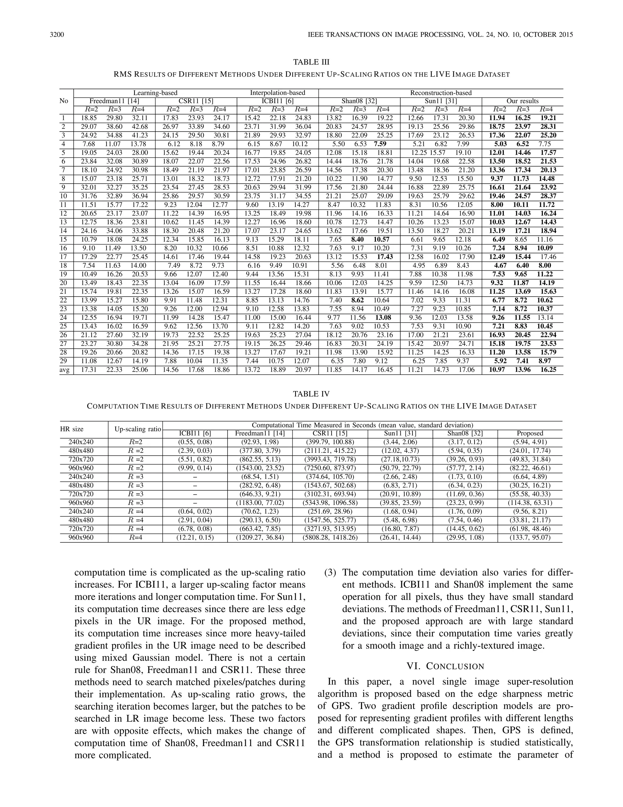
D. Comparison in Computation Time
The computation time of super-resolution methods is mainly
affected by three factors: image content, LR/HR image size,
and up-scaling ratio. The effect of image content can be

13. YAN et al.: SINGLE IMAGE SUPERRESOLUTION BASED ON GPS 3199
TABLE I
THE IMAGE INDEX NUMBERS AND THEIR CORRESPONDING IMAGE NAMES IN LIVE DATABASE [41]
TABLE II
SSIM RESULTS OF DIFFERENT METHODS UNDER DIFFERENT UP-SCALING RATIOS ON THE LIVE IMAGE DATASET
eliminated by making a statistical analysis on large amount
of LR images. Thus only the impacts of LR/HR image size
and up-scaling ratio are discussed in this section.
The reference images adopted in the experiment are from
LIVE database [41]. All the methods are tested under four
HR image sizes (240 × 240, 480 × 480, 720 × 720, and
960 × 960) and three up-scaling ratios (R = 2, 3, 4), where
their corresponding LR image sizes are shown in the second
column of Table IV. For each HR image size and each
up-scaling ratio, 100 LR images are generated by first
randomly selecting an image and then randomly picking up
a region with the LR image size. The computation time is
represented by the mean value and standard deviation of the
100 super-resolution implementations.
The six methods adopted in the comparison are one
interpolation-based method (ICBI11 [6]), two learning-based
methods (Freedman11 [14], and CSR11 [15]), and three
reconstruction-based methods (Shan08 [32], Sun11 [31] and
the proposed method). Shan08 has provided an executable
program on the website [45]. Since there are no public
codes/software for Freedman11 and Sun11, these two methods
are implemented by ourselves, where the parameter configu-
ration are set according to [14] and [31]. The test platform
for ICBI11, Freedman11, CSR11, Sun11, and the proposed
approach is MATLAB R2010a. All the methods are executed
on a computer of Intel Core2 CPU with 2.33 GHz, 1.95GB
memory. The results of computation time are listed in Table IV.
Since ICBI11 can only afford a super-resolution image with
a 2N up-scaling ratio (N is a positive integer), there is not the
computation time of ICBI11 under the up-scaling ratio of 3.
Three basic observations can be drawn from Table IV:
(1) The interpolation-based method has the fastest
computation speed, the learning-based methods need
the longest computation time, and the reconstruction-
based methods is a tradeoff between the two kinds of
methods. Among the reconstruction-based methods,
the computation time of the proposed method is larger
than Shan08 and Sun11 due to the estimation of mixed
Gaussian model.
(2) When the up-scaling factor is fixed, the computation
time of all methods increases as the HR/LR image size
grows. When the HR image size is fixed, the change of

14. 3200 IEEE TRANSACTIONS ON IMAGE PROCESSING, VOL. 24, NO. 10, OCTOBER 2015
TABLE III
RMS RESULTS OF DIFFERENT METHODS UNDER DIFFERENT UP-SCALING RATIOS ON THE LIVE IMAGE DATASET
TABLE IV
COMPUTATION TIME RESULTS OF DIFFERENT METHODS UNDER DIFFERENT UP-SCALING RATIOS ON THE LIVE IMAGE DATASET
computation time is complicated as the up-scaling ratio
increases. For ICBI11, a larger up-scaling factor means
more iterations and longer computation time. For Sun11,
its computation time decreases since there are less edge
pixels in the UR image. For the proposed method,
its computation time increases since more heavy-tailed
gradient profiles in the UR image need to be described
using mixed Gaussian model. There is not a certain
rule for Shan08, Freedman11 and CSR11. These three
methods need to search matched pixeles/patches during
their implementation. As up-scaling ratio grows, the
searching iteration becomes larger, but the patches to be
searched in LR image become less. These two factors
are with opposite effects, which makes the change of
computation time of Shan08, Freedman11 and CSR11
more complicated.
(3) The computation time deviation also varies for differ-
ent methods. ICBI11 and Shan08 implement the same
operation for all pixels, thus they have small standard
deviations. The methods of Freedman11, CSR11, Sun11,
and the proposed approach are with large standard
deviations, since their computation time varies greatly
for a smooth image and a richly-textured image.
VI. CONCLUSION
In this paper, a novel single image super-resolution
algorithm is proposed based on the edge sharpness metric
of GPS. Two gradient profile description models are pro-
posed for representing gradient profiles with different lengths
and different complicated shapes. Then, GPS is defined,
the GPS transformation relationship is studied statistically,
and a method is proposed to estimate the parameter of

15. YAN et al.: SINGLE IMAGE SUPERRESOLUTION BASED ON GPS 3201
GPS transformation relationship automatically. Based on the
transformed GPS, two gradient profiles transformation models
are proposed, which can keep the profile magnitude sum and
profile shape consistent during the transformation. Finally,
the transformed gradients are utilized as priors in the high
resolution image reconstruction. Plenty of experiments are
conducted to evaluate the performance of the proposed method
on subjective visual quality, objective quality, and computation
time. Experimental results show that the proposed approach
can faithfully recover high-resolution image with little
observable artifacts.
REFERENCES
[1] H. S. Hou and H. Andrews, “Cubic splines for image interpolation and
digital filtering,” IEEE Trans. Acoust., Speech Signal Process., vol. 26,
no. 6, pp. 508–517, Dec. 1978.
[2] X. Zhang and X. Wu, “Image interpolation by adaptive 2D autore-
gressive modeling and soft-decision estimation,” IEEE Trans. Image
Process., vol. 17, no. 6, pp. 887–896, Jun. 2008.
[3] F. Zhou, W. Yang, and Q. Liao, “Interpolation-based image super-
resolution using multisurface fitting,” IEEE Trans. Image Process.,
vol. 21, no. 7, pp. 3312–3318, Jul. 2012.
[4] S. Mallat and G. Yu, “Super-resolution with sparse mixing estimators,”
IEEE Trans. Image Process., vol. 19, no. 11, pp. 2889–2900, Nov. 2010.
[5] W. Dong, L. Zhang, R. Lukac, and G. Shi, “Sparse representation based
image interpolation with nonlocal autoregressive modeling,” IEEE Trans.
Image Process., vol. 22, no. 4, pp. 1382–1394, Apr. 2013.
[6] A. Giachetti and N. Asuni, “Real-time artifact-free image upscaling,”
IEEE Trans. Image Process., vol. 20, no. 10, pp. 2760–2768, Oct. 2011.
[7] W. T. Freeman, T. R. Jones, and E. C. Pasztor, “Example-based super-
resolution,” IEEE Comput. Graph. Appl., vol. 22, no. 2, pp. 56–65,
Mar./Apr. 2002.
[8] J. Yang, J. Wright, T. Huang, and Y. Ma, “Image super-resolution
as sparse representation of raw image patches,” in Proc. IEEE Conf.
Comput. Vis. Pattern Recognit., Jun. 2008, pp. 1–8.
[9] K. Zhang, X. Gao, D. Tao, and X. Li, “Multi-scale dictionary for
single image super-resolution,” in Proc. IEEE Conf. Comput. Vis. Pattern
Recognit., Jun. 2012, pp. 1114–1121.
[10] S. Yang, M. Wang, Y. Chen, and Y. Sun, “Single-image super-resolution
reconstruction via learned geometric dictionaries and clustered sparse
coding,” IEEE Trans. Image Process., vol. 21, no. 9, pp. 4016–4028,
Sep. 2012.
[11] H. Yue, X. Sun, J. Yang, and F. Wu, “Landmark image super-resolution
by retrieving web images,” IEEE Trans. Image Process., vol. 22, no. 12,
pp. 4865–4878, Dec. 2013.
[12] M. Ebrahimi and E. R. Vrscay, “Solving the inverse problem of image
zooming using ‘self-examples,”’ in Image Analysis and Recognition.
Berlin, Germany: Springer-Verlag, 2007, pp. 117–130.
[13] D. Glasner, S. Bagon, and M. Irani, “Super-resolution from
a single image,” in Proc. IEEE Int. Conf. Comput. Vis., Sep./Oct. 2009,
pp. 349–356.
[14] G. Freedman and R. Fattal, “Image and video upscaling from local self-
examples,” ACM Trans. Graph., vol. 30, no. 2, pp. 1–12, Apr. 2011.
[15] W. Dong, L. Zhang, and G. Shi, “Centralized sparse representation for
image restoration,” in Proc. IEEE Int. Conf. Comput. Vis., Nov. 2011,
pp. 1259–1266.
[16] J. Ren, J. Liu, and Z. Guo, “Context-aware sparse decomposition for
image denoising and super-resolution,” IEEE Trans. Image Process.,
vol. 22, no. 4, pp. 1456–1469, Apr. 2013.
[17] L. He, H. Qi, and R. Zaretzki, “Beta process joint dictionary learning
for coupled feature spaces with application to single image super-
resolution,” in Proc. IEEE Conf. Comput. Vis. Pattern Recognit.,
Jun. 2013, pp. 345–352.
[18] G. Yu, G. Sapiro, and S. Mallat, “Solving inverse problems with
piecewise linear estimators: From Gaussian mixture models to structured
sparsity,” IEEE Trans. Image Process., vol. 21, no. 5, pp. 2481–2499,
May 2012.
[19] M.-C. Yang and Y.-C. F. Wang, “A self-learning approach to sin-
gle image super-resolution,” IEEE Trans. Multimedia, vol. 15, no. 3,
pp. 498–508, Apr. 2013.
[20] M. Bevilacqua, A. Roumy, C. Guillemot, and M.-L. Alberi Morel,
“Single-image super-resolution via linear mapping of interpolated self-
examples,” IEEE Trans. Image Process., vol. 23, no. 12, pp. 5334–5347,
Dec. 2014.
[21] X. Gao, K. Zhang, D. Tao, and X. Li, “Image super-resolution with
sparse neighbor embedding,” IEEE Trans. Image Process., vol. 21, no. 7,
pp. 3194–3205, Jul. 2012.
[22] T. Peleg and M. Elad, “A statistical prediction model based on sparse
representations for single image super-resolution,” IEEE Trans. Image
Process., vol. 23, no. 6, pp. 2569–2582, Jun. 2014.
[23] X. Gao, K. Zhang, D. Tao, and X. Li, “Joint learning for single-image
super-resolution via a coupled constraint,” IEEE Trans. Image Process.,
vol. 21, no. 2, pp. 469–480, Feb. 2012.
[24] H. Stark and P. Oskoui, “High-resolution image recovery from image-
plane arrays, using convex projections,” J. Opt. Soc. Amer. A, vol. 6,
no. 11, pp. 1715–1726, 1989.
[25] M. Irani and S. Peleg, “Motion analysis for image enhancement: Reso-
lution, occlusion, and transparency,” J. Vis. Commun. Image Represent.,
vol. 4, no. 4, pp. 324–335, Dec. 1993.
[26] B. K. Gunturk, Y. Altunbasak, and R. M. Mersereau, “Color plane
interpolation using alternating projections,” IEEE Trans. Image Process.,
vol. 11, no. 9, pp. 997–1013, Sep. 2002.
[27] R. Fattal, “Image upsampling via imposed edge statistics,” ACM Trans.
Graph., vol. 26, no. 3, p. 95, Jul. 2007.
[28] N. Joshi, C. L. Zitnick, R. Szeliski, and D. J. Kriegman, “Image
deblurring and denoising using color priors,” in Proc. IEEE Conf.
Comput. Vis. Pattern Recognit., Jun. 2009, pp. 1550–1557.
[29] J. Sun, Z. Xu, and H.-Y. Shum, “Image super-resolution using gradient
profile prior,” in Proc. IEEE Conf. Comput. Vis. Pattern Recognit.,
Jun. 2008, pp. 1–8.
[30] J. Sun, J. Zhu, and M. F. Tappen, “Context-constrained hallucination
for image super-resolution,” in Proc. IEEE Conf. Comput. Vis. Pattern
Recognit., Jun. 2010, pp. 231–238.
[31] J. Sun, J. Sun, Z. Xu, and H.-Y. Shum, “Gradient profile prior
and its applications in image super-resolution and enhancement,”
IEEE Trans. Image Process., vol. 20, no. 6, pp. 1529–1542,
Jun. 2011.
[32] Q. Shan, Z. Li, J. Jia, and C.-K. Tang, “Fast image/video upsampling,”
ACM Trans. Graph., vol. 27, no. 5, p. 153, Dec. 2008,
[33] H. Zhang, Y. Zhang, H. Li, and T. S. Huang, “Generative Bayesian
image super resolution with natural image prior,” IEEE Trans. Image
Process., vol. 21, no. 9, pp. 4054–4067, Sep. 2012.
[34] S. Dai, M. Han, W. Xu, Y. Wu, and Y. Gong, “Soft edge smoothness prior
for alpha channel super resolution,” in Proc. IEEE Int. Conf. Comput.
Vis., Jun. 2007, pp. 1–8.
[35] Y.-W. Tai, S. Liu, M. S. Brown, and S. Lin, “Super resolution using edge
prior and single image detail synthesis,” in Proc. IEEE Conf. Comput.
Vis. Pattern Recognit., Jun. 2010, pp. 2400–2407.
[36] D. Krishnan and R. Fergus, “Fast image deconvolution using hyper-
Laplacian priors,” in Proc. NIPS, vol. 22. 2009, pp. 1–9.
[37] D. Krishnan, T. Tay, and R. Fergus, “Blind deconvolution using a
normalized sparsity measure,” in Proc. IEEE Conf. Comput. Vis. Pattern
Recognit. (CVPR), Jun. 2011, pp. 233–240.
[38] K. Zhang, X. Gao, D. Tao, and X. Li, “Single image super-resolution
with non-local means and steering kernel regression,” IEEE Trans. Image
Process., vol. 21, no. 11, pp. 4544–4556, Nov. 2012.
[39] X. Ran and N. Farvardin, “A perceptually motivated three-component
image model—Part I: Description of the model,” IEEE Trans. Image
Process., vol. 4, no. 4, pp. 401–415, Apr. 1995.
[40] T. O. Aydin, M. ˇCadík, K. Myszkowski, and H.-P. Seidel, “Visually
significant edges,” ACM Trans. Appl. Perception, vol. 7, no. 4, p. 27,
Jul. 2010.
[41] Live Database for Image Quality Assessment. [Online]. Available:
http://live.ece.utexas.edu/research/quality
[42] INRIA Person Dataset for Human Detection. [Online]. Available:
http://pascal.inrialpes.fr/data/human/
[43] J. Canny, “A computational approach to edge detection,” IEEE Trans.
Pattern Anal. Mach. Intell., vol. PAMI-8, no. 6, pp. 679–698, Nov. 1986.
[44] W. T. Freeman, E. C. Pasztor, and O. T. Carmichael, “Learning
low-level vision,” Int. J. Comput. Vis., vol. 40, no. 1, pp. 25–47,
Oct. 2000.
[45] The Executable Program of Shan08. [Online]. Available:
http://www.cse.cuhk.edu.hk/~leojia/projects/upsampling/index.html
[46] The Super-Resolution Results of Glasner09. [Online]. Available:
http://www.wisdom.weizmann.ac.il/~vision/SingleImageSR.html
[47] The Super-Resolution Results of Freedman11. [Online]. Available:
http://www.cs.huji.ac.il/~raananf/projects
[48] Z. Wang, A. C. Bovik, H. R. Sheikh, and E. P. Simoncelli, “Image
quality assessment: From error visibility to structural similarity,” IEEE
Trans. Image Process., vol. 13, no. 4, pp. 600–612, Apr. 2004.
[49] A Commercial Product Genuine Fractals. [Online]. Available:
http://genuine-fractals.en.softonic.com/download

16. 3202 IEEE TRANSACTIONS ON IMAGE PROCESSING, VOL. 24, NO. 10, OCTOBER 2015
Qing Yan received the B.E. degree from the China
University of Mining and Technology, Xuzhou,
China, in 2007, and the M.E. and Ph.D. degrees from
Shanghai Jiao Tong University, in 2009 and 2014,
respectively. Her research interests include image
processing, pattern recognition, and intelligent video
analysis.
Yi Xu received the B.S. and M.S. degrees from
the Nanjing University of Science and Technology,
Nanjing, China, in 1996 and 1999, respectively,
and the Ph.D. degree from Shanghai Jiao Tong
University, Shanghai, China, in 2005. She is cur-
rently an Associate Professor with the Department
of Electronic Engineering, Institute of Image
Communication and Network Engineering,
Shanghai Jiao Tong University, Shanghai. Her
research interests include image processing,
intelligent video analysis, and quaternion wavelet
theory and application.
Xiaokang Yang (M’00–SM’04) received the B.S.
degree from Xiamen University, Xiamen, China, in
1994, the M.S. degree from the Chinese Academy
of Sciences, Shanghai, China, in 1997, and the
Ph.D. degree from Shanghai Jiao Tong University,
Shanghai, in 2000. From 2000 to 2002, he was
a Research Fellow with the Centre for Signal
Processing, Nanyang Technological University,
Singapore. From 2002 to 2004, he was a Research
Scientist with the Institute for Infocomm Research,
Singapore. From 2007 to 2008, he visited the
Institute for Computer Science, University of Freiburg, Germany, as an
Alexander von Humboldt Research Fellow. He is currently a Distinguished
Professor of the School of Electronic Information and Electrical Engineering,
and the Deputy Director of the Institute of Image Communication and
Information Processing with Shanghai Jiao Tong University, Shanghai. He has
authored over 200 refereed papers, and has filed 40 patents. His current
research interests include visual signal processing and communication, media
analysis and retrieval, and pattern recognition. He is a member of the Asia-
Pacific Signal and Information Processing Association, a member of Visual
Signal Processing and Communications Technical Committee of the IEEE
Circuits and Systems Society, a member of Multimedia Signal Processing
Technical Committee of the IEEE Signal Processing Society, the Chair
of Multimedia Big Data Interest Group of Multimedia Communications
Technical Committee of the IEEE Communication Society. He was a member
of Editorial Board of Digital Signal Processing. He is also an Associate
Editor of the IEEE SIGNAL PROCESSING LETTERS and the Series Editor
of Communications in Computer and Information Science (Springer).
Truong Q. Nguyen is currently a Professor
with the Department of Electrical and Computer
Engineering, University of California at San Diego,
La Jolla, CA, USA. He has co-authored (with
Prof. G. Strang) a popular textbook entitled
Wavelets and Filter Banks (Wellesley-Cambridge
Press, 1997), and has authored several
MATLAB-based toolboxes on image compression,
electrocardiogram compression, and filter bank
design. He has authored over 400 publications. His
research interests are 3D video processing
and communications and their implementation. He received the
IEEE TRANSACTION in Signal Processing Paper Award (Image and
Multidimensional Processing area) for the paper he co-wrote with
Prof. P. P. Vaidyanathan on linear-phase perfect-reconstruction filter
banks (1992). He received the NSF Career Award in 1995 and is currently
the Series Editor of Digital Signal Processing (Academic Press). He served
as an Associate Editor of the IEEE TRANSACTION ON SIGNAL PROCESSING
from 1994 to 1996, the IEEE SIGNAL PROCESSING LETTERS from
2001 to 2003, the IEEE TRANSACTION ON CIRCUITS AND SYSTEM from
1996 to 1997 and 2001 to 2004, and the IEEE TRANSACTION ON IMAGE
PROCESSING from 2004 to 2005.