Course Project based on SInGAN paper : Reproduce SinGAN results and extend its application to image denoising.

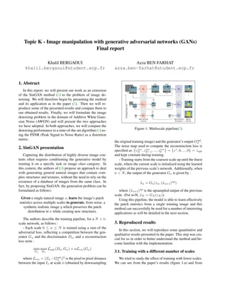
1. Topic K - Image manipulation with generative adversarial networks (GANs)
Final report
Khalil BERGAOUI
khalil.bergaoui@student.ecp.fr
Azza BEN FARHAT
azza.ben-farhat@student.ecp.fr
1. Abstract
In this report, we will present our work as an extension
of the SinGAN method (2) to the problem of image de-
noising. We will therefore begin by presenting the method
and its application as in the paper (2). Then we will re-
produce some of the presented results and compare them to
our obtained results. Finally, we will formulate the image
denoising problem in the domain of Additive White Gaus-
sian Noise (AWGN) and will present the two approaches
we have adopted. In both approaches, we will compare the
denoising performance to a state-of-the-art algorithm (1) us-
ing the PSNR (Peak Signal to Noise Ratio) as a distortion
metric.
2. SinGAN presentation
Capturing the distribution of highly diverse image con-
tents often requires conditioning the generative model by
training it on a specific task or image class category. In
this context, the authors of (2) propose an approach to deal
with generating general natural images that contain com-
plex structures and textures, without the need to rely on the
existence of a database of images from the same class. In
fact, by proposing SinGAN, the generation problem can be
formulated as follows:
Given a single natural image x, learn the image’s patch
statistics across multiple scales to generate, from noise, a
synthetic realistic image y which preserves the patch
distribution in x while creating new structures.
The authors describe the training pipeline, for a N + 1-
scale network, as follows :
- Each scale 0 ≤ n ≤ N is trained using a sum of the
adversarial loss, reflecting a competition between the gen-
erator Gn and the discriminator Dn, and a reconstruction
loss term :
min
Gn
max
Dn
Ladv(Dn, Gn) + αLrec(Gn)
where Lrec = ||In −Gopt
n ||2
is the pixel to pixel distance
between the input In at scale n (obtained by downsampling
Figure 1: Multiscale pipeline(2)
the original training image) and the generator’s output Gopt
n .
The noise map used to compute the reconstruction loss is
specified as :{zrec
N , zrec
N−1, ..., zrec
0 } = {z∗
, 0, ..., 0} = zopt
and kept constant during training.
- Training starts from the coarsest scale up until the finest
scale, where the current scale is initialized using the learned
weights of the previous scale’s network. Additionally, when
n < N, the output of the generator Gn is given by :
x̃n = Gn(zn, (x̃n+1)up
)
where (x̃n+1)up
is the upsampled output of the previous
scale. (For n=N, x̃N = GN (zN )).
Using this pipeline, the model is able to learn effectively
the patch statistics from a single training image and this
method can successfully be used for a number of interesting
applications as will be detailed in the next section.
3. Reproduced results
In this section, we will reproduce some quantitative and
qualitative results presented in the paper. This step was cru-
cial for us in order to better understand the method and be-
come familiar with the implementation.
3.1. Training with a different number of scales
We tried to study the effect of training with fewer scales.
We can see from the paper’s results (figure 1.a) and from

2. ours (figure 1.b) that when we generate samples from mod-
els learnt with a small number of scales (2, 4 and 5), only
general textures are captured. As the number of scales in-
creases, larger structures emerge, as well as the global ar-
rangement of objects in the scene. This is due to the size
of the effective receptive field that is lowest at the coarsest
levels, allowing to capture only fine textures.
(a) paper results
(b) our results
Figure 2: Training with a different number of scales.
3.2. Generating from different scales
The multi-scale architecture of SinGAN allows us to
choose the scale from which we want to generate samples.
At test time, if we generate from the coarsest scale N, we
use random noise as an input. However, if we want to gen-
erate from finer scales n < N, the input used is a downsam-
pled version of the original image. As we can see in figure 2,
changing the scale from which we generate has an impact
on the results. For example, generating from the scale N
does not preserve the global structures of the training image
(the Zebra can have 5 legs, the tree can have 2 trunks,etc),
while generating from finer scales N − 1 and N − 2 allows
to preserve the global structure and changes only fine details
(the shape and pose of the Zebra are preserved and only its
stripe texture changes).
Similar effects are also present in the figures we repro-
duced (images of the cows and the stone) but they are less
interpretable compared to the example of the Zebra.
(a) paper results
(b) our results
Figure 3: Generating random samples from different scales.
3.3. Super resolution
This application consists in increasing the resolution of
an image by a chosen factor s. To do so, SinGAN is trained
on a low resolution input image using a pyramid scale r =k
√
s for k ∈ N. This way, at test time, we upsample the
low-resolution input image by a factor r and we inject it to
the generator at the finest scale. We repeat this k times to
obtain the high-resolution image.
We reproduced the super resolution results of the paper,
where we increase the resolution of the input image by a
factor 4, as shown in figure 4. Our results are very similar
to the paper’s.
Figure 4: Super resolution, with a resolution factor of 4.
The low resolution image is on the left, the paper’s result is
in the middle and ours is on the right.
2

3. 3.4. Paint-to-Image
Transforming a Paint into an Image can be achieved by
training SinGAN on a target image, then feeding a down-
sampled paint into one the coarsest levels (N −1 or N −2).
As we can see in figure 5, we obtain good results where
the output preserves the global structure of the painting and
generates fine details from the target image.
Figure 5: Paper results.
We can also see on figure 6 the impact of the scale to
which we feed the downsampled clipart. In fact, one can
notice that the chosen scale has an impact on the quality of
the output and on the preservation of the global shapes. In
our example, scale N − 2 seems to lead to the result that is
closest to the training image.
Figure 6: Our results.
4. Application to denoising
PS: As of this section, we will adopt the notation used
in the code implementation rather than the paper, in a sense
that we will refer to the coarsest scale as the scale with the
lowest index.
In this section, we will apply SinGAN to the following
problem, assuming a Gaussian Noise n ,→ N(0, σ2
) :
Given a noisy image x = y + n, Generate, the underlying
clean image y
Experimentally, we will proceed by training SinGAN
on the image yt, then during inference, we will construct
a noisy version x = yt + n(σ) and feed it to a generator
Gn at some scale n of the SinGAN. We will conduct
two types of experiments, first yt will represent the clean
image y, then a noisy version of y. The output of the
n-scale Gn will be considered as the denoised image and
will be compared to the original clean image y. We will
conduct the experiments for a wide range of noise standard
deviation σ values in order to assess the limitations of the
application. Since SinGAN trains by learning the patch
statistics of the image, the question we would like to answer
is the following :
Could we benefit from the multi-scale architecture in or-
der to restore the image by separating noise from the learned
patch statistics ?
4.1. Train on a clean image
We start by considering training the model on a clean im-
age (without adding noise) and we use a 6-scale architecture
(the corresponding scale factor parameter is 0.75). At test
time, we choose a scale n and feed a downsampled noisy
image to the generator Gn. We plot in figure 7 the Peak
Signal to Noise Ratio for different values of σ, for different
scales:
Figure 7: Denoising results for different training scales with
a 6-scale architecture. The order of the scales indicated in
the figure is as follows: gen start scale = 6 corresponds to
the finest scale and gen start scale = 0 corresponds to the
coarsest scale.
We observe that denoising is more efficient starting from
the finest scales. Also, intermediate scales seem to general-
ize better for larger noise, and that it leads to the best results
when σ gets large (≥ 35). Note that, in the above figure,
we added G(zopt
) as our baseline as it theoretically repre-
sents the best reconstruction candidate when training on the
clean image, because the reconstruction loss Lrec is exactly
computed using the noise map zopt
as described in section
1 of our report.
In a next step, we trained the model on the same clean
input image using a 13-scale architecture (the correspond-
ing scale factor parameter is 0.85). The below figure shows
that the best results are obtained at intermediate scales (6
and 7). Hence, it seems that increasing the training scales
3

4. (by increasing the scale factor) improves the denoising per-
formance.
Figure 8: Denoising results for different training scales with
a 13-scale architecture. The order of the scales indicated on
the figure is as follows: gen start scale = 13 corresponds to
the finest scale and gen start scale = 0 corresponds to the
coarsest scale.
Finally, we compared the improved PSNR, obtained us-
ing the 13-architecture, with the performance of a-state-of-
the-art denoising algorithm: BM3D(1) on the same noisy
image. Table 1 shows the results where we can see that
BM3D slightly outperforms SinGAN and that the difference
between the PSNRs decreases when σ increases (the image
is more noisy).
σ SinGAN BM3D
10 26.35 30.05
20 24.80 26.02
30 23.47 24.04
40 22.08 22.94
Table 1: PSNR(dB) comparison
However, depending on the size of the training image,
SinGAN could take up to 1.5h, while BM3D takes only
about 5s (in our example) to perform denoising. Moreover,
in practice, we do not have access to the clean image. That
is why we considered a second approach in which we train
the model on a noisy image directly.
4.2. Train on a noisy image
In this section, we consider a more realistic study case
in which we do not have access to the clean image as in
the previous section. The training image therefore consists
of a noisy image obtained by adding AWGN of standard
deviation σ = 30 and we proceed by down-sampling the
image which initially has a 367x585 resolution to obtain a
training image of resolution 157x250. The advantages of
such approach are three fold :
- Down-sampling reduces the noise level: In fact, down-
sampling the image can be equivalent to computing a new
image by averaging neighbour pixels to reduce the resolu-
tion. Such averaging operation helps reduce the noise level.
In particular, in the context of gaussian noise, and assum-
ing independence between the individual pixels, it can be
shown that the noise standard deviation σdown in the down-
sampled image can be expressed as :
σdown = σ ∗
q
Ndown
N where N and Ndown are respec-
tively the number of pixels in the original image and in the
down-sampled one.
- Training time decreases with the resolution of the train-
ing image (this could be interpreted as a result of the com-
putation of the pixel-to-pixel reconstruction loss Lrec). In
fact, we report (Figure Appendix D) the time that takes to
train a single scale on 2000 epochs (using the default config-
uration) for various settings of training image resolutions.
- During inference, we can take advantage of the Super
Resolution mode in order to compensate the down-sampling
operation.
In our case, we compare the results obtained using this
approach, with and without Super Resolution at test time.
The used architecture contains 12-scales and as expected,
the network overfits the training image and learns the noise
pattern. However, interestingly, this occurs at the level of
the finest scales. In fact, we can visualize the output of
the nth
Generator from n = 1 (coarsest scale) to n = 12
(Finest scale). We observe (Figure Appendix B) as we move
from the coarsest to the finest scale, more image details are
learned but also the noise! We find that the 5th
scale pro-
vides the best tradeoff between enough image details and
relatively low noise levels (the image appears smooth but
somewhat blurry).
Quantitatively, this effect can be seen by plotting the
PSNR as a function of the scale:
Figure 9: PSNR vs Scale.
The peak is obtained for the generator G5 (similarly
to the qualitative result) with a value PSNR = 20.9dB.
4

5. Then, we attempt to increase our performance by applying
Super-Resolution as described in section 3.3 (this time only
during inference). By varying the super resolution factor,
the best results were obtained using the same generator G5
using a super-resolution factor ≈ 1.5:
Figure 10: PSNR vs Super-Resolution Factor.
As a result, we obtain an improvement of 1.2dB com-
pared to the situation without using SR, giving us a value
PSNR = 22.10dB. Eventhough we managed to im-
prove our denoising efficiency using SR, we are still out-
performed by state-of-the-art algorithms: For instance
BM3D(1) scores, for the same example (and same σ = 30)
a PSNR = 26.97dB.
5. Conclusion
As we have shown in the previous sections, we have
managed to successfully reproduce most of the results pre-
sented in the paper. Moreover, with respect to applying
SiNGAN to denoising as defined in our report, our denois-
ing methods are still far from state-of-the-art performance.
In order to reduce this gap, other possible research direc-
tions could be explored by :(a) assessing the influence of
SinGAN’s receptive field (in our experiments the receptive
field was equal to 11) on the denoising performance, and
(b): manipulating the loss function by changing the recon-
struction loss term to a perceptual loss term and study the
perception-distortion tradeoff.
References
[1] Marc Lebrun. An analysis and implementation of the bm3d
imagedenoising method. Image Processing On Line, 2012. 1,
4, 5
[2] Tamar Rott Shaham Tali Dekel Tomer Michaeli. Singan:
Learning a generative model from a single natural image.
arXiv:1905.01164v2 [cs.CV], 2019. 1
5

6. Appendix A
Figure 11: Qualitative comparison between our denoising approach(based on the clean training) with state-of the-art BM3D.
Appendix B
Figure 12: Noise is learned at finer scales: At coarser scales, many image details are still missing. As we move to finer scales,
more image details start to appear and then the noise pattern also emerges (in our case at scale 6). In total the architecture
has 12 scales.
6

7. Appendix C
Figure 13: Qualitative comparison between our denoising approach(based on the noisy training) with state-of the-art BM3D.
Appendix D
Figure 14: Time that takes training a single scale over 2000 epochs. The time increases with the training image resolution,
using a fixed architecture across scales (so same number of trainable parameters)
7

8. Appendix E
Figure 15: Failure cases at generating random samples.
8