1. Characterization of Acoustic Band Structure in Layered Composites Subjected to Dynamic
Loading
Jimmy Pan, Ruize Hu, Dr. Caglar Oskay
Civil and Environmental Engineering Department, Vanderbilt University, Nashville, TN
Motivation and Objectives
Motivation
Continuation of a nonlocal homogenization model for bimaterial composite
structures with the purpose of blast and impact mitigation
Examination of the effect of material microstructure and properties on wave
dispersion and attenuation responses
Numerous military and structural applications including cloaking, impact and
blast resistance, and health monitoring
Objectives
Model the bandgap structure arising from the difference in material properties
(e.g. density and modulus of elasticity) of bilayered materials
Define a function of material properties (e.g. impedance and wave velocity)
that approximates a parameter ν used to model bandgap structure
Problem Statement and Approach
Problem Statement
Analyze the dispersion and attenuation characteristics of a bilayer composite
structure experiencing one-dimensional wave propagation
Figure: One dimensional periodic composite structure (Hui 2013)
For each case in a range of material combinations, determine the value of the
parameter ν between 0 and 1 that gives the experimental model the closest fit
to the Floquet-Bloch reference model
ν is a parameter which determines the respective contribution of two nonlocal
equilibrium equations that compose a sixth order dispersion equation (i.e. a
weight factor)
Figure: Effect of ν on Bandgap Model Figure: Dispersion Relation for Aluminum -
Polymer Combination
Research Approach
1. Compose MATLAB script that calculates the ν value resulting in the best fit
for all desired material combinations
2. Plot the best ν values against parameters defined as material properties in
order to give ν physical meaning
3. Curve fit the data to obtain a function that approximates ν
Terminology
Bandgap: the frequency band within which the dynamic response is significantly attenuated.
Arises from interaction between incoming waves and scattered waves due to reflection and
refraction at constituent material interfaces
Attenuation: reduction in the strength of the dynamic response
Nonlocal: in mathematical homogenization theory, refers to defining a mean displacement based
on the macroscale displacements and solving for the mean displacement rather than solving
each equilibrium equation sequentially at each order; only one nonlocal equilibrium equation is
solved
Generating Best Fit ν Data
Minimizing the Objective Function
Objective Function:
Obj = C|y1exp − y1FB| + |y2exp − y2FB|
y1exp: The experimental model’s bandgap initiation point
y2exp: The experimental model’s bandgap endpoint
y1FB: The Floquet-Bloch reference model’s bandgap initiation point
y2FB: The Floquet-Bloch reference model’s bandgap endpoint
C: Weight factor. Set to 1 because an equally weighted objective function yielded the
lowest errors
Used MATLAB’s fminbnd function to minimize Obj and return the corresponding ν value
Range of Material Combinations
Held one layer constant as a specific material and varied the second layer’s material
properties within the desired material class according to the Ashby Materials Selection plot
For example: Aluminum - Polymer
E1 = 68 GPa
ρ1 = 2700 kg/m3
E2 = 1.568 GPa
ρ2 = 1225 kg/m3
α (volume fraction) = 0.5
ˆl (unit cell length) = 0.01 m
The ν value resulting in the best fit for this
scenario was calculated to be 0.3154. To
generate the full set of Aluminum - Polymer
data, set E2 as an array of equally spaced
intervals between 0.08 and 10 GPa, and set ρ2 as
an array of equally spaced intervals between 800
and 2500 kg/m3 Figure: Young’s Modulus (E) vs. Density (ρ) Ashby
Materials Selection Plot (University of Cambridge
Department of Engineering 2002)
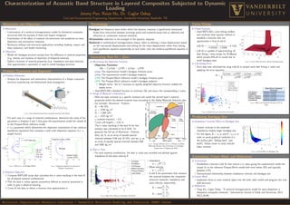
Best ν Data
For each material combination, the best ν value was recorded and plotted against
impedance ˆz and wave velocity ˆc
Figure: Best Fit ν Data as a Function of ˆz and ˆc
Impedance
z =
√
E × ρ
Wave velocity
c = E/ρ
ˆz and ˆc are parameters that measure
the contrast between the composite
structure materials’ impedance and
wave velocity, respectively
ˆz = max(
z1
z2
,
z2
z1
)
ˆc = max(
c1
c2
,
c2
c1
)
Curve Fitting
Fitted Function
Used MATLAB’s curve fitting toolbox
and nonlinear least squares method to
establish a function that can
approximate ν from ˆz and ˆc
ν(ˆz,ˆc) =
1
−0.6181ˆz + 2.559ˆc
+ 0.1161
ν(ˆz,ˆc) is capable of approximating all
best fitting ν data except for Al-Metals,
which proved difficult to model due to
small bandgap sizes Figure: Curve Fitted Function ν(ˆz,ˆc) Overlaying Data
Calculating Error
Error data was calculated by using ν(ˆz,ˆc) to project each best fitting ν value and
applying the error equation:
Ψ =
(y1exp − y1FB)2
+ (y2exp − y2FB)2
y1FB2 + y2FB2
Figure: Overall Error as a Function of ˆz and ˆc
Figure: Mean and Standard Deviation of Error
Data
Predicting Bandgap Size
Impedance Contrast Effect on Bandgap Size
Greater contrast in the materials’
impedances implies larger bandgap size
For this figure, ˆz = z1/z2 and ˆc =c1/c2 in
order to avoid graphical confusion (i.e.
the surface plot ”folding back” over
itself). Values closer to unity indicate
lower contrast
Figure: ˆz and ˆc Effect on Bandgap Size
Conclusions, Future Work, and References
Conclusions
Established a function ν(ˆz,ˆc) that returns a ν value giving the experimental model the
closest fit to the reference Floquet-Bloch model with error below 10% and typically
between 2-5%
Demonstrated relationship between impedance contrast and bandgap size
Future Work
Implement three or more material layers into the sixth order model and progress into core
shell structure
References
Tong Hui, Caglar Oskay. ”A nonlocal homogenization model for wave dispersion in
dissipative composite materials.” International Journal of Solids and Structures, 2013:
50(1):38-48.
Multiscale Computational Mechanics Laboratory / Vanderbilt Multiscale Modeling and Simulation (MUMS) Center