economics

1. Submitted to: Mr. Jospeh Guevarra, PhD. Submitted by: Mark Stephen Pere-ira,MBA
UNIVERSITY OF NEGROS OCCIDENTAL – RECOLETOS
RECOLETOS DE BACOLOD GRADUATE SCHOOL
BACOLOD CITY
DOCTOR OF PHILOSOPHY IN BUSINESS MANAGEMENT
ADVANCED MICROECONOMICS
BM309E 030
MIDTERM EXAMINATIONS
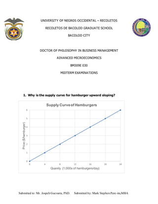
1. Why is the supply curve for hamburger upward sloping?
0
1
2
3
4
5
6
0 4 8 12 16 20 24
Price($/hamburger)
Quanity (1,000s of hamburgers/day)
Supply Curveof Hamburgers

2. Submitted to: Mr. Jospeh Guevarra, PhD. Submitted by: Mark Stephen Pere-ira,MBA
The concepts of supply and demand form the basis of every initial Economics
101 lecture, as well the basis of a market-based economy. Markets are made up of
sellers and buyers, and sellers provide supply to meet buyers’ demand. Supply refers to
the amount of products or services offered by the market, while demand refers to the
amount buyers are willing to purchase at a certain price. Both supply and demand can
be represented visually as curves on a graph – supply slopes upward, while demand
slopes downward.
There are a number of explanations of the direct relationship of supply and price
of hamburgers, including the law of diminishing marginal returns. The law of
diminishing marginal returns explains what happens to the output of hamburgers when
a firm uses more variable inputs while keeping a least one factor of production fixed.
Real capital, such as buildings, machinery, and equipment, is usually the factor kept
fixed when demonstrating this principle.
Economic theory predicts that, when employing these extra variable factors, such
as labour, the marginal returns from each extra unit of hamburger will eventually
diminish.
For a firm which produces hamburgers, its expense for machineries and
equipment is fixed. Extra workers can be hired to increase the output of hamburgers. At
first, the addition of extra workers creates a significant benefit because it becomes
possible to divide up the labour, and for workers to specialise in undertaking one task.
Initially, there are increasing marginal returns to each additional worker.

3. Submitted to: Mr. Jospeh Guevarra, PhD. Submitted by: Mark Stephen Pere-ira,MBA
However, marginal returns will eventually fall because the opportunity to divide
labour and to specialise must eventually ‘dry up’. Gradually, each additional worker
contributes less than the one before so that total output of hamburgers continues to
rise, but at a decreasing rate. The falling marginal returns from each successive worker
leads to a rise in the cost of using them.
Firms need to sell their extra hamburger at a higher price so that they can pay the
higher marginal cost of production. Hence, decisions to supply are largely determined
by the marginal cost of production. The supply curve slopes upward, reflecting the
higher price needed to cover the higher marginal cost of production. The higher
marginal cost arises because of diminishing marginal returns to the variable factors.
2. Why is the demand curve for hamburger downward sloping?
0
1
2
3
4
5
6
0 4 8 12 16 20 24
Price($/hamburger)
Quanity (1,000s of hamburgers/day)
Demand Curve of Hamburgers

4. Submitted to: Mr. Jospeh Guevarra, PhD. Submitted by: Mark Stephen Pere-ira,MBA
When price fall the quantity demanded of a commodity rises and vice versa, other
things remaining the same. It is due to this law of demand that demand curve slopes
downward to the right.
Now, the important question is why the demand curve slopes downward, or in other
words why the law of demand describing inverse price-demand relationship is valid. We
can explain this with marginal utility analysis and also with the indifference
curve analysis.
At higher prices, the quantity of hamburgers demanded is less than at lower
prices. The demand schedule of hamburgers indicates that, typically, there is an inverse
relationship between the price of a product and the quantity demanded. This
relationship is easiest to see in the graph plotted above.
Demand curves generally have a negative slope indicating the inverse
relationship between quantity demanded and price. There are at least three accepted
explanations of why demand curves slope downwards; the law of diminishing marginal
utility, the income effect, and the substitution effect.
One of the earliest explanations of the inverse relationship between price and
quantity demanded for hamburgers is the law of diminishing marginal utility. This law
suggests that as more of a product is consumed, the marginal benefit to the consumer
falls, hence consumers are prepared to pay lesser and lesser. This is because most
benefit is generated by the first unit of a good consumed for it satisfies all or a large
part of the immediate need or desire. A second unit consumed would generate less
utility - perhaps even zero, given that the consumer now has less need or less desire.

5. Submitted to: Mr. Jospeh Guevarra, PhD. Submitted by: Mark Stephen Pere-ira,MBA
With less benefit derived, the rational consumer is prepared to pay rather less for the
second, and subsequent, units, because the marginal utility falls.
While total utility continues to rise from extra consumption of hamburgers, the
additional utility from each hamburger falls. If marginal utility is expressed in a
monetary form, the greater the quantity consumed the less the marginal utility and the
less value derived - hence the rational consumer would be prepared to pay less for
another unit of hamburger.
The income and substitution effect can also be used to explain why the demand
curve slopes downwards. If we assume that money income is fixed, the income effect
suggests that, as the price of a hamburger falls, real income - that is, what consumers
can buy with their money income - rises and consumers increase their demand.
Therefore, at a lower price, consumers can buy more hamburgers from the same
money income, and, ceteris paribus, demand will rise. Conversely, a rise in price will
reduce real income and force consumers to cut back on their demand.
In addition, as the price of hamburger falls, it becomes relatively less expensive.
Therefore, assuming other alternative products like hotdog sandwich stay at the same
price, at lower prices the hamburger appears cheaper, and consumers will switch from
the hotdog sandwich to hamburgers.
It is important to remember that whenever the price of hamburger changes, it
will trigger both an income and a substitution effect.

6. Submitted to: Mr. Jospeh Guevarra, PhD. Submitted by: Mark Stephen Pere-ira,MBA
3. What does the equilibrium price and quantity of hamburger in the
market look like?
The equality of quantity demanded and quantity supplied is an indicator of the
established equilibrium. In the graph showing the demand and supply curves above, the
point of intersection of these two curves is the point of equilibrium. This is because at the
point of intersection the demand and supply become equal to each other. In this case, the
SUPPLYDEMAND
MARKET EQUILIBRIUM
0
1
2
3
4
5
6
0 4 8 12 16 20 24
Price($/hamburger)
Quanity (1,000s of hamburgers/day)
Demand and Supply ofHamburgers
EQUILIBRIU
M
QUANTITY
EQUILIBRIU
M PRICE

7. Submitted to: Mr. Jospeh Guevarra, PhD. Submitted by: Mark Stephen Pere-ira,MBA
equilibrium price is $3 per hamburger while the equilibrium quantity is 12,000 hamburgers
per day.
Equilibrium means a state of no change. Evidently, at the equilibrium price, both
buyers and sellers of hamburgers are in a state of no change. Technically, at this price,
the quantity of hamburgers demanded by the buyers is equal to the quantity of
hamburgers supplied by the sellers. Both market forces of demand and supply operate in
harmony at the equilibrium price.
Graphically, this is represented by the intersection of the demand and supply curve.
Further, it is also known as the market clearing price. The determination of the
market price is the central theme of microeconomics. That is why the microeconomic
theory is also known as price theory.
A detailed look at the above supply and demand schedule reveals a bag full of
information about the market. Most importantly, we can observe that the demand and
supply become equal at a price of 3. Thus 3 is the equilibrium price.
Next, note how the impact on price is downwards when the price of hamburger is
too high for the buyer’s taste, which is the portion above the equilibrium price. Lastly,
again the impact on price is upwards when it is too low for the supplier’s taste. To point
out, the price tends to move towards the equilibrium mark.
Both consumers and sellers do not want to shift from the equilibrium price. In that
case, the equilibrium price can change only when there is a change in both demand and
supply. An increase in only demand or only supply is taken by horns by a self-adjusting
mechanism.

8. Submitted to: Mr. Jospeh Guevarra, PhD. Submitted by: Mark Stephen Pere-ira,MBA
When the price of hamburgers increases, the sellers flock to the market with their
products for an opportunity to earn higher profits. This creates a condition of excess
supply, ultimately leading to a surplus of the hamburgers in the market. In order to sell
this surplus, the sellers have to reduce the price. Effectively, the price continues to fall
until it reaches the equilibrium level.
When the price of hamburger decreases, the consumers sense an opportunity to
buy the product at a lower price. This creates gives birth to excess demand of
hamburgers. Consequentially, there starts brewing a situation of competition among the
buyers which eventually pushes up the price. Eventually, the price continues to rise until it
reaches the equilibrium level.
The supply and demand schedule mentioned above is an indicator of all these
processes.