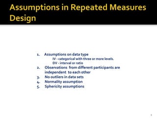
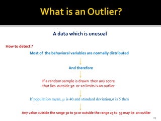
Presented by
Dr.J.P.Verma
MSc (Statistics), PhD, MA(Psychology), Masters(Computer Application)
Professor(Statistics)
Lakshmibai National Institute of Physical Education, Gwalior, India
(Deemed University)
Email: vermajprakash@gmail.com
1. Assumptions on data type
IV - categorical with three or more levels.
DV - interval or ratio
2. Observations from different participants are
independent to each other
3. No outliers in data sets
4. Normality assumption
5. Sphericity assumptions
2
 The type I error increases
 Power of the test decreases
 Internal and External validities are at stake
3
Some assumptions are design issues
and
Some can be tested by using SPSS or other software
Lets Learn to use SPSS first
4
5
This Presentation is based on
Chapter 3 of the book
Repeated Measures Design
for Empirical Researchers
Published by Wiley, USA
Complete Presentation can be accessed on
Companion Website
of the Book
Step 1: Activate SPSS by clicking on the following command sequence.
Start All Programs IBM SPSS Statistics
Figure 3.1 Option for creating/opening data file
6
Step 2: Prepare data file
 Choose the option “Type in data” if data file is prepared first time
 Choose the option “Open an existing data source” if existing
data file to be used
Step 3: Prepare data file in two steps
a. Define all variables by clicking on “VariableView”
b. Feed data by clicking on “DataView”
7
i. Define short name of the variable under column Name
 Name should not start with number or any special character
 Only special character that can be used is underscore “_”
 If the name consists of two words it must be joined with underscore
ii. Define full name of the variable, the way you feel like under Label
iii. If variable is nominal define coding under heading Values
iv. Define data type of each variable in Measure
Step 1
Figure 3.2 Option for defining variables and coding 8
Step 2
Figure 3.3 Format for data feeding
9
 By skewness and Kurtosis
 By Means of Kolmogorov-Smirnov test and Shapiro-Wilk test
 Normal Q-Q plot
10
Most of the statistical tests are based upon the concept of normality
To test the normality
Check the significance of
 Skewness
 Kurtosis
11
One of the characteristics of normal distribution
3
2
2
3
1



Symmetrical distribution
How to measure skewness?
Skewed curves
Positively skewed curve Negatively skewed curve
01 
01 
- ∞ + ∞ - ∞ + ∞
11 
01 
12
Positively skewed curve
- ∞ + ∞
X: 3,2,3,2,4,6,3,5,5,4,6,4,3,8,90
Mean=14.6
Remark: Most of the scores are less than the mean
value
Negatively skewed curve
- ∞ + ∞
X: ,3,2,65,68,66,70,67,64,65,69,72,70
Mean=58.3
Remark: Most of the scores are more than the mean value
01 
01 
13
Skewness is significant if its value is more than two times its standard error
)3n)(1n)(2n(
)1n(n6
)(SE)Skewness(SE 1



)(SE2 11 
14
2
2
4
2



One of the characteristics of the normal distribution
How to measure the spread of scores? 322 
02 
02 
02 
15
Kurtosis is significant if its value is more than two times its standard error
)(SE2 22 
)5n)(3n(
1n
)(SE2)(SE)Kurtosis(SE
2
12



16
Self image (in nos.) Height(in ft.)
24.00 5.40
30.00 5.50
22.00 5.50
42.00 5.60
38.00 5.60
21.00 5.60
24.00 5.70
30.00 5.70
22.00 5.70
24.00 5.70
23.00 5.80
23.00 5.80
28.00 5.80
24.00 5.90
21.00 5.90
45.00 6.00
24.00 5.80
23.00 5.50
28.00 5.60
30.00 5.60
22.00 5.70
28.00 5.70
24.00 5.70
45.00 5.80
42.00 5.90
Analyze Descriptive statistics Explore
Figure 3.4 Initiating commands for testing normality
and identifying outliers
17
Figure 3.5 Option for selecting variables and detecting outliers
Check for
identifying
outliers through
Box-Plot
Click on for
outlier options
18
Check this
option for
generating
outputs of
Shapiro test
and Q-Q plots
Click on for
normality test
and QQ Plots
option
Figure 3.6 Options for computing Shapiro-Wilk test and the Q-Q plot
19
Table 3.3 Tests of normality
_________________________________________________
Kolmogorov-Smirnov Shapiro-Wilk
Statistics df Sig. Statistic df Sig.
_________________________________________________
Self image .269 25 .000 .785 25 .000
Height .140 25 .200 .963 25 .484
_________________________________________________
If Shapiro-Wilk statistic is not significant (p>.05) then normality exists.
Result: Height is normally distributed but the self image is not
Criteria ofTesting
20
Shapiro-Wilk Test is appropriate for small
sample sizes (n< 50) but can be used for
sample sizes as large as 2000
 In large sample more likely to get significant results
Limitation
21
Normal Q_Q plot for self image Normal Q_Q plot for height
Figure 3.7 Normal Q-Q Plot for the data on self image and height
22
A data which is unusual
How to detect ?
Most of the behavioral variables are normally distributed
And therefore
If a random sample is drawn then any score
that lies outside 3σ or 2σ limits is an outlier
If population mean, µ is 40 and standard deviation,σ is 5 then
Any value outside the range 30 to 50 or outside the range 25 to 55 may be an outlier
23
24
To buy the book
Repeated Measures Design
for Empirical Researchers
and all associated presentations
Click Here
Complete presentation is available on
companion website of the book

Testing Assumptions in repeated Measures Design using SPSS

  • 1.
    Presented by Dr.J.P.Verma MSc (Statistics),PhD, MA(Psychology), Masters(Computer Application) Professor(Statistics) Lakshmibai National Institute of Physical Education, Gwalior, India (Deemed University) Email: vermajprakash@gmail.com
  • 2.
    1. Assumptions ondata type IV - categorical with three or more levels. DV - interval or ratio 2. Observations from different participants are independent to each other 3. No outliers in data sets 4. Normality assumption 5. Sphericity assumptions 2
  • 3.
     The typeI error increases  Power of the test decreases  Internal and External validities are at stake 3
  • 4.
    Some assumptions aredesign issues and Some can be tested by using SPSS or other software Lets Learn to use SPSS first 4
  • 5.
    5 This Presentation isbased on Chapter 3 of the book Repeated Measures Design for Empirical Researchers Published by Wiley, USA Complete Presentation can be accessed on Companion Website of the Book
  • 6.
    Step 1: ActivateSPSS by clicking on the following command sequence. Start All Programs IBM SPSS Statistics Figure 3.1 Option for creating/opening data file 6
  • 7.
    Step 2: Preparedata file  Choose the option “Type in data” if data file is prepared first time  Choose the option “Open an existing data source” if existing data file to be used Step 3: Prepare data file in two steps a. Define all variables by clicking on “VariableView” b. Feed data by clicking on “DataView” 7
  • 8.
    i. Define shortname of the variable under column Name  Name should not start with number or any special character  Only special character that can be used is underscore “_”  If the name consists of two words it must be joined with underscore ii. Define full name of the variable, the way you feel like under Label iii. If variable is nominal define coding under heading Values iv. Define data type of each variable in Measure Step 1 Figure 3.2 Option for defining variables and coding 8
  • 9.
    Step 2 Figure 3.3Format for data feeding 9
  • 10.
     By skewnessand Kurtosis  By Means of Kolmogorov-Smirnov test and Shapiro-Wilk test  Normal Q-Q plot 10
  • 11.
    Most of thestatistical tests are based upon the concept of normality To test the normality Check the significance of  Skewness  Kurtosis 11
  • 12.
    One of thecharacteristics of normal distribution 3 2 2 3 1    Symmetrical distribution How to measure skewness? Skewed curves Positively skewed curve Negatively skewed curve 01  01  - ∞ + ∞ - ∞ + ∞ 11  01  12
  • 13.
    Positively skewed curve -∞ + ∞ X: 3,2,3,2,4,6,3,5,5,4,6,4,3,8,90 Mean=14.6 Remark: Most of the scores are less than the mean value Negatively skewed curve - ∞ + ∞ X: ,3,2,65,68,66,70,67,64,65,69,72,70 Mean=58.3 Remark: Most of the scores are more than the mean value 01  01  13
  • 14.
    Skewness is significantif its value is more than two times its standard error )3n)(1n)(2n( )1n(n6 )(SE)Skewness(SE 1    )(SE2 11  14
  • 15.
    2 2 4 2    One of thecharacteristics of the normal distribution How to measure the spread of scores? 322  02  02  02  15
  • 16.
    Kurtosis is significantif its value is more than two times its standard error )(SE2 22  )5n)(3n( 1n )(SE2)(SE)Kurtosis(SE 2 12    16
  • 17.
    Self image (innos.) Height(in ft.) 24.00 5.40 30.00 5.50 22.00 5.50 42.00 5.60 38.00 5.60 21.00 5.60 24.00 5.70 30.00 5.70 22.00 5.70 24.00 5.70 23.00 5.80 23.00 5.80 28.00 5.80 24.00 5.90 21.00 5.90 45.00 6.00 24.00 5.80 23.00 5.50 28.00 5.60 30.00 5.60 22.00 5.70 28.00 5.70 24.00 5.70 45.00 5.80 42.00 5.90 Analyze Descriptive statistics Explore Figure 3.4 Initiating commands for testing normality and identifying outliers 17
  • 18.
    Figure 3.5 Optionfor selecting variables and detecting outliers Check for identifying outliers through Box-Plot Click on for outlier options 18
  • 19.
    Check this option for generating outputsof Shapiro test and Q-Q plots Click on for normality test and QQ Plots option Figure 3.6 Options for computing Shapiro-Wilk test and the Q-Q plot 19
  • 20.
    Table 3.3 Testsof normality _________________________________________________ Kolmogorov-Smirnov Shapiro-Wilk Statistics df Sig. Statistic df Sig. _________________________________________________ Self image .269 25 .000 .785 25 .000 Height .140 25 .200 .963 25 .484 _________________________________________________ If Shapiro-Wilk statistic is not significant (p>.05) then normality exists. Result: Height is normally distributed but the self image is not Criteria ofTesting 20
  • 21.
    Shapiro-Wilk Test isappropriate for small sample sizes (n< 50) but can be used for sample sizes as large as 2000  In large sample more likely to get significant results Limitation 21
  • 22.
    Normal Q_Q plotfor self image Normal Q_Q plot for height Figure 3.7 Normal Q-Q Plot for the data on self image and height 22
  • 23.
    A data whichis unusual How to detect ? Most of the behavioral variables are normally distributed And therefore If a random sample is drawn then any score that lies outside 3σ or 2σ limits is an outlier If population mean, µ is 40 and standard deviation,σ is 5 then Any value outside the range 30 to 50 or outside the range 25 to 55 may be an outlier 23
  • 24.
    24 To buy thebook Repeated Measures Design for Empirical Researchers and all associated presentations Click Here Complete presentation is available on companion website of the book