Activity-Based Rail Freight Costing A Model For Calculating Transport Costs In Different Production Systems

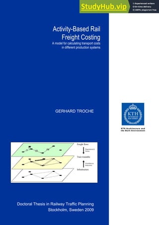
GERHARD TROCHE
Doctoral Thesis in Railway Traffic Planning
Stockholm, Sweden 2009
Infrastructure
Train timetable
Freight flows
Possibilities&
Restrictions
Requirements &
Desires

KUNGL
IGA T
EKNISKA HÖGSKOL
AN
Roya l Institute of T
e c hnolog y
Division for T
ra nsporta tion & L
og istic s
Ra ilwa y Group
T
RIT
A- T
EC- PHD 09- 002
ISSN 1653- 4468
ISBN 13:978- 91- 85539- 35- 2
Ac tivity- Ba se d Ra il Fre ig ht Costing
A mode l for c a lc ula ting tra nsport c osts
in diffe re nt produc tion syste ms
G e rha rd T
roc he
Do c to ra l T
he sis
Sto c kho lm, Fe b rua ry 2009

Gerhard Troche
- 2 -
© 2009 Gerhard Troche
gerhard@infra.kth.se
Division for Transportation & Logistics
- Railway Group -
S – 100 44 STOCKHOLM
Sweden
www.infra.kth.se
Printed in Sweden by Universitetsservice US AB, Stockholm 2009

Activity-Based Rail Freight Costing
- 3 -

Gerhard Troche
- 4 -
Innehåll
Preface 7
Summary 9
1 Introduction 17
1.1 Background 17
1.2 The need for information on railway costs 23
1.3 Goals and purpose 26
1.4 Delimitations 28
2 Literature review 31
2.1 Introductory remarks 31
2.2 General theory of costs and cost calculation 33
2.3 Transport cost models for rail freight 51
3 Methodology 67
3.1 Research approach 67
3.2 Selection of activities and cost items to be depicted 71
3.3 Model validation 75
3.4 Methods of data collection 78
4 Structuring the rail freight system 83
4.1 Products and production systems 83
4.2 Operating principles for freight trains 90
4.3 Changing organizational structures in the railway sector 99
5 Cost allocation in the rail freight system 103
5.1 Allocating costs in a specific transport system 103
5.2 Handling the joint and common cost problem 108
5.3 The Empty Wagon Problem 111
6 General structure of the model 115
6.1 Overview 115
6.2 The infrastructure level 117
6.3 The train service level 121
6.4 The freight-flow level 122
6.5 Utilization model 123
7 Databases in EvaRail 125
7.1 Overview 125

- 5 -
7.2 Freight flow database 128
7.3 Infrastructure database 129
7.4 Train database 131
7.5 Commodity database 133
7.6 Vehicle database 134
7.7 Load unit database 136
7.8 “Interconnecting” databases 137
7.9 Other cost databases 139
8 Cost calculation in EvaRail 143
8.1 Overview 143
8.2 Wagon capital or leasing costs 148
8.3 Wagon maintenance and service costs 152
8.4 Locomotive capital or leasing costs 154
8.5 Locomotive maintenance and service costs 159
8.6 Driver costs 161
8.7 Energy costs 163
8.8 Infrastructure charges 168
8.9 Activity costs 172
8.10 Other costs 178
8.11 Empty running factors 184
9 Examples of results in EvaRail 189
9.1 Applications with analysis of cost structure 189
9.2 Unit train Mora-Gävle 190
9.3 Wagonload Helsingborg–Sundsvall – heavy freight 193
9.4 Wagonload Helsingborg–Sundsvall – light freight 197
9.5 Liner train system and dual-power locomotives 199
9.6 Intermodal traffic 201
9.7 Express freight trains 203
10 Discussion and conclusions 205
10.1 Methodological issues 205
10.2 Model results 209
10.3 Further model development and improvements 211
11 Literature 215

- 7 -
Preface
This thesis is the concluding report of the research project ‘Cost and
supply model for rail freight’, carried out between 1999 and 2008 at the
Centre for Research and Education in Railway Engineering at the
Division of Transportation & Logistics at the Royal Institute of
Technology (KTH) in Stockholm.
My principal supervisor has been Bo-Lennart Nelldal, adjunct professor
in train traffic planning at KTH, assisted by Arne Jensen, professor in
transport economics at the School of Business, Economics and Law at
Göteborg University. All material in this thesis has been produced by the
author. The project was financed by Banverket, the National Swedish Rail
Administration, via KTH Railway Group.
My sincere thanks are due to all the people who contributed to the
project with information, knowledge and valuable comments. It was a
pleasure for me to find people with a genuine experience of, interest in
and fascination with railways and freight transport. I would also like to
thank my supervisors Bo-Lennart Nelldal and Arne Jensen for their
invaluable help – and sometimes also their patience – without which this
thesis would not have been possible. Finally, for their patience and
understanding, my special thanks go to my parents, all my friends and
especially to those people who accompanied me and formed a part of my
life during the years I worked in this project and who reminded me that
there is a life even outside cost models and railway yards.
Stockholm, January 2009
Gerhard Troche

- 9 -
Summary
Europe’s railways are at present undergoing far-reaching changes. The
restructuring takes different forms in different countries and the pace also
varies. One common denominator, however, is the growing influence of
market forces on development, principally of freight traffic, in almost the
whole of Europe. Freight traffic, as opposed to a large proportion of
passenger traffic, is operated – and forced to maintain its position –
under commercial conditions. The restructuring also affects the cost
structure and – which is important in connection with the present thesis
– how this can be illustrated in a cost model for rail freight traffic.
The above means that costs and revenues, and the relationship between
the two, are two key aspects that ultimately determine the railway’s future
position in the freight transport market. Knowledge in these areas is
therefore important, partly for the railway companies themselves, but also
for other parties in the sector who are in some way affected by, and/or
take decisions that have relevance for freight traffic. These might for
example be transportation customers, infrastructure operators, politicians
and researchers.
This project focuses on the cost side, where knowledge is today
inadequate, not least outside of the railway companies. Figure 1 illustrates
fields where cost information is used and needed.
A cost model that illustrates the railway’s many and rather complex
production systems would thus satisfy many different players’ need for
cost information. The aim of this project was to develop such a model
and use it in selected case studies to analyse the cost structure and the
effect of changes in the railway system, thus increasing understanding of
what factors are the cost-drivers in the railway system.
The cost model has been delimited to constitute a business economics
model from a train operator’s perspective. External costs are thus not
calculated. The model calculates transportation costs at the flow level. By
being able to handle several flows, the model also makes it possible to
calculate costs for larger transport systems, in which cases the

Gerhard Troche
- 10 -
delimitation of such a system may vary depending on the user of the
information (for example train operator, transportation customer, etc).
Detailed information on all these flows is, however, a requirement.
Pricing
Pricing
Vehicle investments
Vehicle investments
Operations planning
Operations planning
Business strategies
Business strategies
Legislation
Legislation
Infrastructure investments
Policy strategies
Policy strategies
Subsidies
Subsidies
Transport mode choice
Logistics planning
Logistics planning
Socio-economic analyses
Model development
Model development
Evaluation of trp.-systems
Cost understanding
Cost understanding
TOCs
(Train Operating
Companies)
TOCs
(Train Operating
Companies)
Government and
public administrations
Government and
Shippers,
Freight Forwarders
Shippers,
Freight Forwarders
Infrastructure
Managers
Infrastructure
Managers
Scientific researchers
and consultants
and consultants
Need of
cost information
Need of
cost information
Fields where cost information is needed Actors requiring cost information
Demand
Pricing
Pricing
Vehicle investments
Vehicle investments
Operations planning
Operations planning
Business strategies
Business strategies
Legislation
Legislation
Policy strategies
Policy strategies
Subsidies
Subsidies
Logistics planning
Logistics planning
Model development
Model development
Cost understanding
Cost understanding
TOCs
(Train Operating
Companies)
TOCs
(Train Operating
Companies)
Government and
Government and
Shippers,
Freight Forwarders
Shippers,
Freight Forwarders
Infrastructure
Managers
Infrastructure
Managers
and consultants
and consultants
Need of
cost information
Need of
cost information
Fields where cost information is needed Actors requiring cost information
Demand
Figure: Fields where information on costs in rail freight is needed and
players who require information (G.Troche)
The model was developed with a view to being able to illustrate different
production methods. It is thus not limited to a certain kind of traffic or
production arrangement. This means that the model in this sense is a
general one, which also opens up for using the model to evaluate new
production methods.
The model also provides a basis for calculating transportation prices; the
costs, however, are only one (albeit important) factor in pricing
transportation. The other important factor is the market price, which is
determined by the competitive situation. It is, however, reasonable to

- 11 -
assume that in a longer perspective there is a strong linkage between
transportation prices and transportation costs. By setting a profit margin,
based on an assessment of the competitive situation, a user of the model
can thus also calculate a transportation price.
The project was conducted in six steps:
1) Literature analysis
2) Mapping of production systems in rail freight traffic
3) Identification of activities, resources and costs
4) Definition of cost allocation principles for shared costs
5) Construction and programming of the model
6) Validation and calibration of the model
The literature review showed that few detailed transportation cost models
exist for railways. The models often only illustrate certain production
methods. The lack of transportation cost models for railways and the
shortcomings in the few models that do exist can partly be explained by
the complexity of the railways’ production methods that is much greater
than for practically all other types of transport. This makes it very
difficult to adapt by any simple means a model for truck transportation,
for example, to also suit rail transportation. Another important reason is
the difficulty involved in obtaining relevant cost data because the
necessary data is to a large extent confidential. This fact also explains why
information about the models is sometimes very scanty. On the other
hand, these shortcomings also illustrate the need for a general model.
The ABC (Activity Based Costing) model was identified as a suitable type
of model for calculating transportation costs. Most existing models are
also of this type. Compared to TCS (Traditional Cost Accounting), ABC
models have the advantage that most of them are especially suitable for
operations with high overhead costs, strongly diversified products and
complex production structures, conditions that apply to the railways to a
very high degree.
The mapping of the railways’ production systems showed a great many
different systems (figure 2). This project also included systems that may
be brought into use in the future. Each individual system can itself be
fairly complex, but the complexity of rail freight traffic as a whole is
increasing, not least because the systems are not clearly delimited – and
consequently, in a model, are not delimitable – against each other. One
single transportation assignment may pass through different production

Gerhard Troche
- 12 -
systems on its way between consigner and consignee and/or during
empty trips.
Production system s
Production system s
Trainload
Trainload
Train operating
system s
Train operating
system s
Wagonload
Wagonload
Combined Traffic
Combined Traffic
High-speed rail freight
Junction system
Junction system
Direct trains
Direct trains
Unit trains
Unit trains
Hub-and-spoke
Hub-and-spoke
Group trains
Group trains
Shuttle trains
Shuttle trains
Liner trains
Liner trains
Rolling stock
Rolling stock
Locomotives
Locomotives
Wagons
Wagons
Multiple units
Multiple units
I nfrastructure
I nfrastructure
Lines
Lines
Marshalling yards
Marshalling yards
Local yards
Local yards
Industrial sidings
Industrial sidings
Intermodal
terminals
Intermodal
terminals
Maintenance
facilities
Maintenance
facilities
Personnel
Personnel
Administrative
Administrative
Onbord (drivers)
Onbord (drivers)
Yard & terminal
Yard & terminal
Other resources
( Energy,
…)
Other resources
( Energy,
…)
Custom ized products
”Albatros”
”Albatros”
”Steelbridge”
”Steelbridge”
”Arctic Rail Express”
”PaperSolution”
”PaperSolution”
”…”
”…”
”TECO”
”TECO”
”Orient Freight Express”
General products
General products
”Trainload”
”Trainload”
”Wagonload”
”Wagonload”
”Combined Traffic”
”High-speed rail freight”
Production system s
Production system s
Trainload
Trainload
Train operating
system s
Train operating
system s
Wagonload
Wagonload
Combined Traffic
Combined Traffic
Junction system
Junction system
Direct trains
Direct trains
Unit trains
Unit trains
Hub-and-spoke
Hub-and-spoke
Group trains
Group trains
Shuttle trains
Shuttle trains
Liner trains
Liner trains
Rolling stock
Rolling stock
Locomotives
Locomotives
Wagons
Wagons
Multiple units
Multiple units
I nfrastructure
I nfrastructure
Lines
Lines
Marshalling yards
Marshalling yards
Local yards
Local yards
Industrial sidings
Industrial sidings
Intermodal
terminals
Intermodal
terminals
Maintenance
facilities
Maintenance
facilities
Personnel
Personnel
Administrative
Administrative
Onbord (drivers)
Onbord (drivers)
Yard & terminal
Yard & terminal
Other resources
( Energy,
…)
Other resources
( Energy,
…)
”Albatros”
”Albatros”
”Steelbridge”
”Steelbridge”
”PaperSolution”
”PaperSolution”
”…”
”…”
”TECO”
”TECO”
General products
General products
”Trainload”
”Trainload”
”Wagonload”
”Wagonload”
Figure: Clarification of the terms “products” and “production
systems” (Gerhard Troche)
The approach chosen to handle this in the model is to break down the
production systems into activities. Many activities occur in several
systems. A production system is thus a result of a specific combination of
activities and what characterizes them. No production system is thus
specified in the model, but the activities in each respective chain. If the
user adds several flows, the production systems thus grow on the basis of
how the user specifies the transportation arrangements. This has the
advantage that the definitions and the bases for dividing the production

- 13 -
systems can then be chosen freely dependent of the purpose of the
analysis without this affecting the model’s cost calculations.
Trainload Wagonload Combined
Traffic
High-speed
rail freight
Train hauling + + + +
Shunting o ++ o o
Marshalling - ++ - -
Loading/unloading of
freight in/on/from
wagon
+ + - +
Transloading of freight
between wagon and
truck
+ + - o
Transloading of
Loading Unit between
wagon and truck
- - ++ o
Transloading of
Loading Unit between
wagon and wagon
- - + -
++ very common
+ Common
o Seldom
- Never of almost never
Table: Activities in the rail freight system and in which production
systems these occur. (G.Troche)
Cost information about resources and activities have primarily been
obtained through interviews with experts. This type of information is not
normally available from open, printed sources – at least not as primary
sources. Some data has also been able to be obtained from industry
journals.
Shared costs have been allocated according to the following criteria or
combinations of criteria: (1) time, (2) distance, (3) weight, (4) number of
wagons/vehicles, (6) number of load round trips. By splitting up the costs
as far as possible, a relatively accurate distribution of the costs can be
made. The user can, for example, distribute part of the maintenance costs
by distance, part by time and yet another part by the number of round
trips. An attempt has been made to keep the need to distribute shared

Gerhard Troche
- 14 -
costs to a minimum by applying, where possible and meaningful, a
bottom-up principle when calculating costs, which means that the costs
are then direct costs.
The model consists of three “levels”, where the lowest is made up of the
infrastructure, i.e. the track network, consisting of nodes and links. There
is thus a network in the model that is used to calculate distance and
specify train supply and transport flows, which are the other two levels.
The model contains an automatic route assignment, but it is possible to
determine the route manually as well; the train supply is input manually.
Infrastructure
Train services
Freight flows
Possibilities &
Restrictions
Requirements &
Demand
Infrastructure
Train services
Freight flows
Possibilities &
Restrictions
Requirements &
Demand
Infrastructure
Train services
Freight flows
Possibilities &
Restrictions
Requirements &
Demand
Figure: The three levels in the model (G. Troche)
The model was validated and calibrated through discussions of output
data and model structure with experts. The model has subsequently been
applied in a number of fictive, yet realistic, transport concepts to test the
model’s technical functionality and in an exemplifying manner analyse the
effects of different improvement measures in the railway system.
Examples of measures that have been studied include higher axle loads
and bigger loading gauge and the introduction of new traction in the
form of dual-power locos. For these, the cost effects were quantified for
specific flows. The results of these calculations have also been discussed
with experts and were included in the calibration work.
The project has thus resulted in a model that is able to illustrate and cost
complex transport chains, including complex chains, in the railway
system. The most important future development opportunities lie in
integrating automatic route allocation for empty-running locomotives, to
be able to handle systems with many dispersed flows (e.g. in the

- 15 -
wagonload system) more easily, and an improved resource utilization
model. Interfaces also need to be developed to other models, e.g. demand
forecast models and transport choice models. A combined cost and
demand model or model system would constitute a powerful tool for
quantifying both cost and demand effects.
The most important conclusion from the calculations that have been
performed using the model is that there are two approaches that can be
used to improve the railways’ competitiveness:
− Give the railways better possibilities to utilize economies of scale,
principally in the form of higher axle loads, a bigger loading gauge
and longer/heavier trains. This does not in principle require any
system changes, “merely” an increase in the present maximum
values of the above parameters.
− Introduce new production systems such as liner trains in order to
reduce the costs at each end of the transport chain and to widen
the market by covering even more disperse goods flows. This also
assumes new innovative vehicle concepts such as dual-power
locomotives and new transhipment technologies for small-scale
low-cost terminals.
Resource utilization has a great impact on transportation costs in all
production systems. The implementation of some of the proposals
mentioned above could contribute to a better resource utilization.

- 17 -
1 Introduction
1.1 Background
From development hitherto and the present situation of rail freight in
Europe, it can be concluded that there is an urgent need to take both
short-term and long-term measures to improve rail freight’s profitability,
performance and competitiveness.
In 1970, the railways in Europe (EU 15) had a market share of 31% of
total freight transportation measured in ton-kilometres. Road traffic
accounted for 54% at that time and domestic shipping transported the
remaining 15%. By 1995, the railways' market share had fallen to 15%,
while that of road haulage had increased to 77% and shipping’s share had
fallen to 8%. Over the course of little more than three decades, the
railways' market share has been halved.
During the last decade rail’s market share in the enlarged European
Union (EU 27) has been rather stable, seen for Europe as a whole.
However, the development is not any longer as uniform as it has been
before in a smaller EU, when almost all countries showed a general
downward trend for rail freight.
Looking more closely at the present situation – also including the new
EU members – it can be observed that rail’s market share in most new
member states is still significantly higher than in the rest of Europe.
However the transition from planned economy to market economy has
resulted in heavy losses for rail, often accelerated by a lack of ability – and
maybe sometimes even a lack of willingness – on the part of the member
states to adapt their railways to the new conditions, regardless of whether
it is a matter of infrastructure, organization, finances or culture.
In the old EU member states the development isn’t uniform neither and
several countries now show a significant positive trend for rail. Generally
countries with a deregulated rail freight market and strong intramodal
competition show – thanks to the positive effects of these measures on
costs and service quality – an increase in rail freight, while countries less

Gerhard Troche
- 18 -
committed to deregulation of the rail freight market still continue their
downward trend.
In Germany rail freight ton-kilometres have grown continuously by
almost 50% from 2001 to 2007 and increased its market share from
15,7% to 17,3%. In Great Britain rail freight has increased by more than
70% within little more than a decade from 13,1 billion ton-kilometres
1994/95 to 22,2 billion ton-kilometres 2006/07 and helds now a market
share of 11% compared to 9% before. In Sweden rail freight ton-
kilometres reach an all-time high in 2007 and were 16% higher than 2000;
the market share is stable on a compared to other European countries
very high level of 23%. On a European level rail freight ton-kilometre
have increased by almost 14% from less than 390 billion ton-kilometre in
2002 to more than 430 billion ton-kilometres in 2006.
Modal split ton-kilometres EU-27 1995 - 2006
0%
20%
40%
60%
80%
100%
1995 1996 1997 1998 1999 2000 2001 2002 2003 2004 2005 2006
market
share
in
percent
Sea
Inland Waterway
Road
Rail
Figure 1.1: Performance (Data: EU-DG TREN / Eurostat, 2007)
However, seen in a global perspective the situation in Europe is still
characterized by relatively low market shares for rail and high market
shares for road (see fig.1.3). There are, of course, many explanations for
the high market share in other parts of the world, however, the fact that
rail has a much higher market share in many different parts of the world
with widely varying geographical conditions, traffic patterns and
organizational and political frameworks indicate that there still is a
considerable unexploited market potential for rail in Europe.

- 19 -
Rail freight ton-kilometres EU-27 2000 - 2006
350
360
370
380
390
400
410
420
430
440
2000 2001 2002 2003 2004 2005 2006
billion
ton-kilometres
Figure 1.2: Development of rail freight ton-kilometres 2000-2006 in EU-27.
(Data source: EU-DG TREN / Eurostat, 2007)
Rail and road market shares
0%
10%
20%
30%
40%
50%
60%
70%
80%
EU-27 USA Australia Russia China
percent
of
ton-kilometres
Rail
Road
Figure 1.3: Rail and road market share in different world regions, total
market comprises rail, road, internal waterways and pipelines,
for Australia even coastl shipping (EU, Russia: 2006; USA,
Australia, China: 2005) (Data source: ALLIANZ FÜR
SCHIENE, 2008)

Gerhard Troche
- 20 -
A strategy to break a negative trend for rail or to strengthen the
foundation for a sustainable turnaround has to address both the supply
and the demand side of rail freight. The services offered by the railway
companies have to meet today’s customer requirements and the services
have to be produced efficiently to make them cost-competitive. Higher
productivity combined with greater attractiveness can improve
profitability for rail freight.
Improved
profitability
Improved
profitability
PRODUCTION
Resource
optimization
Increased
productivity
Lower
expenses
Better
offer
Increased
attractiveness
Higher
revenue
MARKET
Improved
profitability
Improved
profitability
PRODUCTION
Resource
optimization
Increased
productivity
Lower
expenses
Better
offer
Increased
attractiveness
Higher
revenue
MARKET
Figure 1.4: A strategy for profitability (Source: Sparmann 1997, in
German)
The challenge is to fill the strategy above with concrete content and to
identify suitable measures. There is no lack of ideas for improving rail
freight’s prospects. Two approaches can be distinguished, based on the
perception that the railway market is surrounded – and limited – by both
technical and economic restrictions (which to some degree are
interdependent), and recognition of the fact that the market price can
scarcely be influenced to any larger extent by the railways, since it is set in
practice by its competitors, in most cases road haulage. The approaches
must therefore focus on the cost side. One approach is to reduce the unit
costs of production resources by both taking advantage of increased
competition on the resource side and implementing new production
methods; another is to achieve economies of scale by (re-)moving
technical restrictions in the form of loading gauges, axle and metre loads,
train lengths, etc. (fig. 1.5).

- 21 -
Economies of scale
EUR
Production costs
Market price
Technical restrictions
(loading gauges, axle loads,
train lengths, …)
Economical limit
(break even-point)
Goal:
Enlarging the railfreight market /
Improving profitability
… by removing
technical restrictions to
realize economies of scale
… by reducing unit
costs of production
resources to lower
break even-point
Approaches to enlarge the railfreight market
and improve profitability
Economies of scale
EUR
Production costs
Market price
Technical restrictions
(loading gauges, axle loads,
train lengths, …)
Economical limit
(break even-point)
Goal:
Enlarging the railfreight market /
Improving profitability
… by removing
technical restrictions to
realize economies of scale
… by reducing unit
costs of production
resources to lower
break even-point
Approaches to enlarge the railfreight market
and improve profitability
Fig. 1.5: Approaches to enlarge the rail freight market and improve
profitability. (Gerhard Troche)
This study focuses on the cost effects of technical and operational
improvements in the railway system, thereby not underestimating the
necessity of measures on the organizational and political level. Measures
on the technical/operational level and those on an
organizational/political level are often to some extent interconnected
with each other. The latter are important when it comes to implementing
technical and operational measures.
Technical improvements refer to changes in the physical resources in the form
of wagons, locomotives, etc. A certain locomotive class may for example
be replaced by a new, “better” locomotive with different technical
characteristics. Operational improvements refer to how the physical resources
are deployed, for example how the trains run (routes, speeds, train
formation, train lengths, stopping pattern, etc.).
In general, it can be said that operational changes can be implemented
faster and can consequently give quicker economic effects – within 1-2
years but often within weeks. Technical improvements often take longer

Gerhard Troche
- 22 -
to implement, typically from one year up to several years. They also often
entail higher investments.
There has been a tradition in the railway sector to analyse technical
improvements in the first place from a technical point of view, i.e. to look
at the technical feasibility and performance, while many times
disregarding economic aspects.
However, in an increasingly liberalized and competitive freight transport
market – and growing in ability and reluctance on the part of states to
cover financial holes in the budgets of their railway companies – it is
natural that the railway companies are paying increasing attention to the
economic effects of their decisions. The need to adopt an integrated
approach when looking at certain measures – taking into account both
technical and economic aspects – is today widely accepted. This of course
also holds true for the new private entrants in the rail freight market.
They are forced to adopt clear business-oriented perspectives from the
very outset.

- 23 -
1.2 The need for information on railway
costs
From the trend to run railways as a business on a commercial basis arises
the need for detailed information about costs in the rail freight system.
An understanding of costs and knowledge about cost-drivers are
becoming essential in business and policy decisions. They are a key factor
for the successful management of a railway company. This is especially
true since railways are faced with the need to modernize their production
systems in order to meet today’s and tomorrow’s customer requirements,
something which often requires substantial (initial) investments.
There is thus a need for a tool that can predict the economic effects of technical and
operational improvements in the railway system.
Cost information and understanding is needed 1
− to identify money makers or money losers
− to take resource allocation decisions
− to plan and control operations and activities
− to find economic break-even points
− to compare different options
− to discover opportunities for cost improvement
− to prepare and actualize business plans
− to improve strategic decisions making
Potential users of a cost model for rail freight and/or its results can be
found in a number of different target groups (see even fig. 1.6):
− Train operating companies
− Government and public administrations
− Shippers
− Infrastructure Managers
− Scientific researchers
Table 1.1 below contains a list of fields in which these groups may use
the model as a decision-support tool.
1 BERRY, L.E. (2005), completed

Gerhard Troche
- 24 -
Liberalization of rail
freight market
freight market
Costs become
essential in business
and policy decisions
Costs become
Problem
- Lack of tools/
models to support
decision-making
- Difficulties to
identify cost-driving
factors
- Lack of tools/
models to support
decision-making
- Difficulties to
factors
Research project
Research project
Effect
Cause
freight market
freight market
Costs become
Costs become
Problem
- Lack of tools/
models to support
decision-making
- Difficulties to
factors
- Lack of tools/
models to support
decision-making
- Difficulties to
factors
Research project
Research project
Effect
Cause
Figure 1.6: Justification and positioning of project (G.Troche)
Train operating
companies
Government and
public
administrations
Shippers Infrastructure
Managers
Scientific
researchers
Pricing
Investments
Operations
Business
strategies
Legislation
Transport
infrastructure
development
Subsidies
Policy strategies
Choice of
transport
mode
Logistical
planning
Socio-economic
analysis
Infrastructure
investments
Policy strategies
Model
development
(demand
forecast)
Evaluation of
transport
systems
Cost
understanding
Table 1.1: Users of rail freight cost information and fields in which they
may use the model as a decision-support tool.(G.Troche)
Forecast models for freight transport often comprise some form of sub-
model for calculation of transport costs. However, these models are only
to a very limited extent useful as a decision-support toll, especially when
it becomes necessary to depict changes in the rail freight system with
major system-wide impact on costs and cost structures. A fundamental
problem with these models is that much of the data used in them
− is often not calculated within the model, but put in as primary
input data, and/or
− is quantified on the basis of often quite uncertain assumptions.
There is thus a great risk that this data will either become very
”conservative”, in the sense that it is based on a status quo assumption or
alternatively on a trend extrapolation of development hitherto; or that
major changes are assumed, but on relatively inexact grounds, allowing
the results to appear to be a ”what would happen if…” scenario, rather

- 25 -
than answering the question ”why would it happen?” – or, by extension,
”how likely is this scenario?”.
Consequently, in order to describe the railways’ opportunities in a
dynamic perspective, i.e. taking into account more extensive changes in
the rail supply as a result of new production methods, improved technical
solutions and operational performance, etc, it is necessary to have cost
information about both different current and possible future rail freight production
systems.
Today, there is no such information – or tool which could produce this
information – publicly available, which would make it possible to
systematically analyse and compare transport costs in different rail freight
production systems or in transport chains where rail cooperates with
other transport modes.
Pricing
Pricing
Vehicle investments
Vehicle investments
Operations planning
Operations planning
Business strategies
Business strategies
Legislation
Legislation
Policy strategies
Policy strategies
Subsidies
Subsidies
Logistics planning
Logistics planning
Model development
Model development
Cost understanding
Cost understanding
TOCs
(Train Operating
Companies)
TOCs
(Train Operating
Companies)
Government and
Government and
Shippers,
Freight Forwarders
Shippers,
Freight Forwarders
Infrastructure
Managers
Infrastructure
Managers
and consultants
and consultants
Need for
cost information
Need for
cost information
Pricing
Pricing
Vehicle investments
Vehicle investments
Operations planning
Operations planning
Business strategies
Business strategies
Legislation
Legislation
Policy strategies
Policy strategies
Subsidies
Subsidies
Logistics planning
Logistics planning
Model development
Model development
Cost understanding
Cost understanding
TOCs
(Train Operating
Companies)
TOCs
(Train Operating
Companies)
Government and
Government and
Shippers,
Freight Forwarders
Shippers,
Freight Forwarders
Infrastructure
Managers
Infrastructure
Managers
and consultants
and consultants
Need for
cost information
Need for
cost information
Fig. 1.7: Fields in which cost information on rail freight is required and
its main users (G. Troche)

Gerhard Troche
- 26 -
1.3 Goals and purpose
In the previous chapter a need for cost information was identified. This
need can be addressed by a cost model. The advantage of a model, in
contrast to benchmarking (case) studies for example, is that it can be
designed in a way, which makes it generally applicable to rail freight. It
can satisfy the demands of different users and has the advantage of
showing a connection between input and output.
The goal of this work is thus to develop a model, which makes it possible
to enhance the understanding of costs in rail freight and to analyse
possible ways to improve the profitability and/or cost competitiveness of
the rail freight system.
The model to be developed has been given the working name EvaRail –
standing for Model for Economic evaluation of rail freight services.
The model aims to describe the supply side of freight transportation by
rail on a detailed level. The model should deliver cost data for door-to-
door transportation of specific (single or recurrent) shipments. At the
same time, the model has to satisfy a requirement to be general and to be
able to depict transportation in (almost) every production system, both
those used today and potential future production systems.
The purpose of the project is to address the need for information of the
different actors as they are identified in the previous chapter, 1.2. This
purpose can be concretized as follows:
− For scientific researchers and consultants working with modelling
and forecasting, the primary purpose of the model is to deliver
input data for transport choice and freight forecasting models.
− For train operators, government and public administrations, and
infrastructure managers, the main purpose of the model will most
likely be to evaluate the economic effects of technical or
operational measures that aim to improve the performance of the
railway system. This can also be relevant for scientific researchers
working with more applied research.
Finally, the model may also serve as an instrument to calculate transport
costs for alternative transport solutions, which addresses the needs of
shippers.

- 27 -
In this project there was no hypothesis to be verified or disproved. The
aim was rather to create a tool – in the form of a supply and cost model –
which in its turn can be used to test hypotheses, for example about the
efficiency of measures to improve the rail freight production system.

Gerhard Troche
- 28 -
1.4 Delimitations
EvaRail is a business-economic, activity-based cost model calculating
costs from the view of a train operator. Under the reasonable assumption that
there exists a connection between production costs in rail freight and the
prices charged to the customers, EvaRail, by adding a profit margin, is
also able to calculate transport costs from a shipper’s point of view.
The scope of a business-economic model is influenced by the
organizational structure of the sector. In the railway industry – as well as
in other industries – this structure has changed over time, and is still
changing, and there also exist considerable differences between different
countries and railway companies. The liberalization of rail freight in
Europe has led to the creation of new private railway companies with a
variety of different business models. At the same time the earlier state
railways have reorganized themselves and adopted business goals,
management methods and organizational structures from the private
sector. In addition, a general trend towards outsourcing has increased the
variety of organizational models in the rail freight sector. There is no
homogeneous structure within the sector and that typical train operating
company does not exist. EvaRail is designed in such a way that it to a
certain degree can adapt to different organizational models. How the
organizational structure affects the depiction of the rail freight
production system is dealt with in more detail in chapter 4.3.
No external costs or effects are included in the model, as long as they are
not internalized in monetary form, i.e. charged to the train operator. It is
not necessary to include external costs since they do not affect the train
operators’ pricing and consequently not the customers’ transport costs
either. Since business-economic costs are also part of a socio-economic
calculation it is, however, highly conceivable that EvaRail can deliver
input data for a socio-economic calculation. It could also be included as a
sub-model in a socio-economic model. The creation of such a socio-
economic model, however, lies outside the scope and intention of this
project.
In EvaRail, emphasis has been put on a detailed depiction and calculation
of rail transport and multimodal road/rail transport chains. The model
calculates transport costs on a flow level. Calculations can be made of
one or several specific flows. It is possible to calculate the costs for a
whole production system, if all flows in a system are known and specified

- 29 -
in detail by the user. This, however, requires comprehensive information
on a large number of flows. Exceptions are large-volume regular flows
(system flows), for which dedicated systems can be established –
normally trainload services.
A production method, which is not yet possible to properly depict in the
model is a combination of passenger and freight transport on the same
train. It would be possible to adapt the model without too big efforts to
cover even this situation, if any need should arise (which, however, is
rather unlikely). In this context is can be mentioned, that – if this should
be done – the model then, in principle, would be able to calculate
production cost in pure rail passenger system as well, including complex
production system with direct wagons.
It should also be emphasized again that this project deals with the cost
side of rail freight. Costs represent only one side of the economic effects
of measures taken to improve the rail freight system. The other side
comprises revenues. These are not part of this project and are
consequently not calculated in the model. A costing model is thus only
one tool for decision-making; it should be complemented by a revenue
model depicting willingness to pay for certain improvements. In the long
term it would be desirable to integrate these models.

- 31 -
2 Literature review
2.1 Introductory remarks
The literature review comprises two parts: In the first part (chapter 2.2) a
number of transport cost models for rail freight are presented. In the
second part (chapter 2.3) the categorization of costs and typical problems
encountered in the development of cost models are discussed. In this
way, the literature review both gives a reference frame for the new model
and identifies problems, which have to be dealt with in the development
of the new model.
When it comes to the first part – the presentation of cost models for rail
freight –the number of pure rail freight (or multi-mode) cost models is
quite limited. Cost models are often integrated in mode choice models,
which in their turn can form part of transport prognosis models. The
reason for this is that costs/prices are an important criterion for the
choice behaviour of shippers. For this reason alone, almost every
transport choice model has necessarily to comprise some form of
transport cost calculation.
However, this does not mean that all transport choice models are
included in this overview. Many transport choice models only contain a
very simple and rough calculation of transport costs. Even a simple
multiplication of transport distance with a net-tonne-kilometre cost –
maybe the most rudimentary calculation of transport costs, which is
possible – in a transport choice model, can in a strict formal meaning be
considered as a “cost model”. However, in the following overview only
models are included which comprise a slightly more sophisticated
transport cost calculation and where the transport cost calculation itself is
an important aim of the model. The model (or its cost module) should be
able to calculate the effects of changes in the rail freight production
system. This requires that the production system is depicted in the model,
at least roughly.
A complication in this part of the work has been that most cost models –
irrespective of whether they form part of transport choice or demand

Gerhard Troche
- 32 -
forecast models or are free-standing cost models – for natural reasons
contain confidential data. Furthermore, many cost models are only
intended for internal use, for example within railway companies. Thus
their existence is sometimes not even known to a broader public nor
within academic circles. Other models have been developed for
commercial use by consulting companies. Even these are for
understandable reasons not too interested in revealing all too detailed
information about their models. For these reasons it has been difficult to
obtain more detailed information about many of the models – this
difficulty not only concerns the input-data, but also the model structure
and the calculation principles.

- 33 -
2.2 General theory of costs and cost
calculation
2.2.1 Cost concepts and categorizations
Costs and cost structures can be described in different ways. In the
following a number of categorizations, which can be found in literature
are presented. Many of these categorizations show similarities and in
many cases the differences are rather in terminology than in definitions.
The purpose of this overview is to help the reader to relate different
terminology used in different contexts to each other.
The categorization of costs used in this dissertation follows – as far as is
applicable – the one presented in figure 2.1.
Direct and Indirect Costs
A common way to is to distinguish between Direct costs and Indirect costs.
The latter can in their turn be divided into Joint costs and Common costs (see
figure 2.1).2
Direct costs can be allocated directly to the production of a certain
product. Allocation of direct costs is consequently “simple” since it is not
necessary to share them between different products.
However, in many cases – and this is especially true in the case of railway
services – many activities are shared between different products. Exactly
what are direct cost and what are indirect costs depends not only on the
price of the activities concerned and the characteristics of the rail service,
but also on what is considered to be the “product”. If for example a
shuttle train service between two container terminals is considered one
product (and the rolling stock and the rolling stock deployed in this train
service is not used for any other duties), then the capital cost of the
rolling stock are direct costs. If, however, the “product” is the transport
of goods in one specific goods flow – of several goods flows using the
train – these have to be regarded as indirect costs.
2 Comp. e.g.: ANIANDER, BLOMGREN, ENGWALL (1998)

Gerhard Troche
- 34 -
All costs
Direct costs Indirect costs
Joint costs Common costs
All costs
Direct costs Indirect costs
Joint costs Common costs
Figure 2.1: Systematization of certain cost terms according to OXERA
(2005).(Graphic: G.Troche)
Common costs – as one type of indirect costs – arise when an activity is
shared voluntarily between two or more products. This means that the
producer chooses to share these activities, normally because it is
economically advantageous. By doing so he may for example achieve
positive scale effects or synergy effects.
Joint costs arise when activities have to be shared in the delivery of a
product, i.e. when they are inseparable. This means that the producer
cannot choose whether or not to share these costs.
An example may serve to illustrate the difference between joint and
common costs: “A train carries commuters into the city early in the
morning and returns nearly empty for a second trip. The seats in the first
and second class carriages share common costs: the carriages have been
linked together for convenience. However, the seats on the upward and
downward journeys share joint costs: the delivery of upward and
downward services is inseparable from another - the train has to travel in
both directions.”3
Translated to freight this means that different wagons in a (wagonload)
train share common costs, while the wagons’ return trip entails joint
costs.
3 OXERA(2005), p.7

- 35 -
The same source also deals with the question of allocating common and
joint costs. Generally it is easier to allocate common costs than joint
costs. In the case of common costs, the underlying activities, their costs
and the cost drivers would be identified and allocated to each product
according to their consumption. In the example above the costs for
traction power and the working time of on-board personnel would be
shared between first and second class passengers accordingly.
The allocation of Joint costs he considers far more problematic, which is
exemplified in OXERA(2005): “A work-study would indicate that the
cost of the upward and downward journeys are similar (the only
difference between a full and empty train being the trivial cost of issuing
tickets). Yet the train only runs for the benefit of commuters, so the
principle of causality would suggest that this group should bear almost
the full cost and the return journey be treated as a by-product and bear
the negligible incremental cost. But should this principle hold in the
evening when the commuters return and theatre-goers undertake
expeditions in the opposite direction? The latter would use the train and
should therefore share the costs of its operation, lowering the costs for
the home-bound commuters.”4
It should be mentioned that the problem of empty trains is highly
relevant in the case of freight traffic: While inbound and outbound
commuter train services certainly show varying load factors, trains are
seldom completely empty. There are normally at least some passengers to
which costs could be allocated. In freight, however, there is often no load
at all for the return run; wagons – and in the case of unit-trains even
whole trainsets – run almost always empty for a part of a turnaround. It
shows also that cost allocation principles are not necessarily
straightforwardly transferable between passenger and freight.
The Baumol-Willig rule5 states that the allocated costs should be no
greater than the stand-alone cost and no less than the incremental cost.
Otherwise joint production would not continue and the benefits of the
economy of scope will be lost; the same effect would arise if the allocated
costs exceed the revenue from a particular product.
KAPLAN even suggests using Ramsey pricing, meaning that indirect
costs should be allocated to products in inverse proportion to their price
4 OXERA(2005), p.7
5 ERGAS, H., RALPH, E.: Pricing Network Interconnection: Is the Baumol-Willig rule the
right answer?, 1996

Gerhard Troche
- 36 -
elasticity - or – as he expresses it in common parlance: “Load the costs
onto those who have little choice but to pay”.6
Fixed and Variable Costs
Characteristic of railways is that many resources are indivisible or –
within certain limits – fixed. This is true even if we do not consider
infrastructure. A high portion of costs is therefore fixed and independent
of transport quantity.
The figure below illustrates a classification of fixed and variable costs. Of
the cost categorizations presented in this chapter this appears to be the
most complete one. For this reason this categorization and its
terminology has also been used in this dissertation.
All costs
Fixed costs Variable costs
Var. tracable
costs
Var. common
costs
Fixed traceable
costs
Fixed common
costs
All costs
Var. tracable
costs
Var. common
costs
Fixed traceable
costs
Fixed common
costs
Fig. 2.2: Systematization of Fixed and Variable costs.7,8
The marginal costs for rail traffic can be calculated with different time
horizons – from adding one ton of freight when loading a wagon, to
investing in new rolling stock with up to more than a year of realization.
The costs for adding one ton of freight – given that the transport capacity
of a wagon is not already reached – is close to zero.
The next step is to add a wagon, which already exists, to an already
scheduled train. This can be done with a horizon of some days. The
6 KAPLAN (2001)
7 NN (2007)
8 CRUM, R.L., GOLDBERG, I. (1998), p. 94

- 37 -
marginal costs would be energy costs, infrastructure fees and
maintenance.
After this the next step would be to arrange a new train departure with
already existing rolling stock. This is possible with a horizon of some
weeks to months. In addition to the costs mentioned above costs for
personnel (man-hours) have to be added to calculate the marginal costs
(assuming that personnel costs are considered to be variable!).
With a time horizon of more than a year, new rolling stock could be
acquired. This may also result in a necessity to invest in new maintenance
facilities and administration. In this case the marginal costs of a train
operating company are almost 100%. When the time horizon is extended
still further – from several years up to decades - a need may also arise for
the infrastructure manager to invest in new infrastructure, e.g. yards and
terminals, or – in an extreme case – new railway lines. In this case, the
marginal costs of the railway system as a whole are approaching 100%.
A further step is taken if terminal costs are affected, which is conceivable
over a period of at least six months. The change is then of such a
magnitude that more personnel need to be taken on for shunting and
switching.
The problem of low short-run marginal costs is especially critical in
pricing decisions. A train operating company that always sets its prices
according to its short-run marginal costs would never be able to cover its
total costs even in the long run. Marginal cost pricing should therefore be
used very carefully and only selectively by train operating companies; it is
only viable if there are market segments where a price higher than total
costs can be achieved.
Specific and Unit costs
The Regulatory Costing Model of the Canadian Transportation Agency
distinguishes between Specific and Unit costs. Both are Variable costs, as
can be seen from the figure below, which shows the cost categorization
used in this model.

Gerhard Troche
- 38 -
All costs
Specific costs Unit costs
Figure 2.3: Systematization of costs according to the Regulatory Costing
Model of the Canadian Transportation Agency. (Source:
CANADIAN TRANSPORT AGENCY)
The differences between specific and unit costs are explained as follows:
“Specific costs are those costs which can be directly attributed to the traffic
or service for which costs are to be determined (for example, crew
wages).”9 In the CTA-model (see chapter 2.3.7) Specific costs are used
whenever:
- costs are 100% variable;
- the expense is directly related to the traffic movement or service
for which costs are being determined; and
- the collection of expense data permits the cost to be identified to
specific segments of the rail operation.
“Unit costs are costs, which are common to all railway traffic and services.
[…] A unit cost represents a mathematical relationship between two
variables: railway expenses (dependent variables) and levels of output
(independent variables). System-wide unit costs are used to assign
common costs to services.
Unit costs are developed through one of two techniques. If the common
cost is deemed to be 100% variable with the system workload statistics to
9 CTA CANADIAN TRANSPORT AGENCY (2006)

- 39 -
be used for cost allocation, the unit cost is developed from the direct
relationship between expenses and workloads. This is called direct analysis.
If the common cost is deemed to be less than 100% variable with the
associated workload statistic or is dependent on two or more workload
statistics, regression analysis (simple or multiple) is normally used. […] A
geographical cross-section of costing data input is required in order to
ensure that costs are truly representative of the railway's system in total.
Regression analysis, be it simple or multiple, is the most widely-used tool
to estimate the fixed and variable costs and to separate the causal effects
of different workloads on grouped expenses (cost complexes).”10
Figure 2.4 gives a further overview of different cost terms and cost
classification principles.11 All three categorization principles cover the
total costs and can be used in parallel. Consequently the cost terms are
overlapping.
Output
Cost allocation principle
Action
Costs
Variable
costs
Fixed
costs
Direct
costs
Indirect
costs
Incremental
costs
Joint
costs
Classification principle Terminology
Output
Cost allocation principle
Action
Costs
Variable
costs
Fixed
costs
Direct
costs
Indirect
costs
Incremental
costs
Joint
costs
Classification principle Terminology
Figure 2.4: Three principles for classification of total costs (Source:
ANIANDER, BLOMGREN, ENGWALL, et.al.. (1998), p. 153)
2.2.2 Principles of cost calculation
Top-down versus bottom-up approach
There are two principally different approaches to calculate the costs for a
certain activity:
• a top-down approach and
• a bottom-up approach
10 CTA CANADIAN TRANSPORT AGENCY (2006)
11 ANIANDER, BLOMGREN, ENGWALL, et al. (1998)

Gerhard Troche
- 40 -
To clarify these terms two examples may be given:
Example I: When using the top-down approach to calculate the staff
costs for the traction, they would be calculated by dividing the total costs
for driver wages in a railway company by the number of driving hours of
all drivers in that company.
A bottom-up approach would be to multiply the number of driver
working-hours for a certain activity by the gross salary per driver-hour.
Example II: When using the top-down approach to calculate the energy
costs for a certain activity, the total traction-related energy costs in a
railway company would be divided by the total train-kilometres (or gross
ton-kilometres or whatever unit of measurement is considered suitable)
this railway company produces during a given period, giving the energy
cost per train-kilometre.
A bottom-up approach would be to calculate the energy consumption for
that activity using a suitable formula which takes into account running
resistance, air resistance, losses, etc. and then multiplying the calculated
energy consumption, suitably expressed in kWh, by the actual working
price per kWh.
Which of the approaches is used in the model depends partly on what
data are available.
Generally a bottom-up approach is preferable for the following reason:
In the top-down approach, there is no longer any direct connection to
the factors causing and determining the costs; instead, the total costs are
simply distributed over some measurement units (train-kilometres,
working hours, tons, etc), although no linear connection necessarily exists
at all.
For example, when calculating infrastructure charges for a train, these can
of course, easily be calculated by dividing a railway company’s total
annual infrastructure charges by the total train-kilometres, although in
reality they might be charged per gross-ton-kilometre or vice versa.
This means that values obtained through a top-down approach are valid
only for the current production of rail freight, and that they are correct
only for an ”average” transport, i.e. average train size, average speed,
average rolling stock productivity, average driver utilization, etc. It is
therefore not, or at least not to the same extent and with the same
precision, possible to quantify effects of differences or changes in the

- 41 -
relevant factors, as the starting point in the top-down approach is the
total costs and not the cost-determining factors.
A bottom-up approach makes it easier to take into consideration specific
characteristics of a transport, as well as changes in the relevant cost-
determining factors, as the following examples illustrate:
When calculating energy costs for example, a bottom-up approach makes
it possible to take into account the weight of the train and if it is running
at high or low speed, while the top-down approach normally only
calculates the costs on the basis of the average energy consumption per
train-kilometre, irrespective of the speed and weight.
Another example would be infrastructure charges. In some countries
these are different on different lines. A bottom-up approach makes it
possible to calculate these costs in a way that takes into account whether
the train in running on a line with low charges or on an ”expensive”
route.
However, there are also problems connected to the bottom-up approach,
mainly practical ones:
− The bottom-up approach demands much more and more detailed
input data, which may not be available. This also applies in
principle to the top-down approach, but there is normally less
data and it is consequently less likely that they will not be
available.
− The amount of data necessary for a calculation increases and
might make the model less user-friendly.
In spite of these problems, the bottom-up approach has been applied as
far as reasonably possible.
Input data and compatibility of data
So far this chapter has presented a number of different cost
categorizations and cost terms. A cost model uses much input cost data
which belong to one of the categories presented above. Knowing which
category certain cost data belong may help to improve understanding of
the model, but for the quality of the model results it is at least as
important to know the exact definition of each piece of cost data
information. The important difference between defining cost categories and
defining specific cost data information is that the developer or user of a

Gerhard Troche
- 42 -
model is quite free in his definition of cost categories – and can thus
follow scientifically accepted definitions more or less without any
problem – while he is totally dependent on the definition of primary cost
data information as it is given in the sources he uses. Apart from the
problem that the exact definition in these – mostly non-scientific –
sources is not always given, he also has to take into account, since he will
normally use information from different sources, the fact that the exact
definition of “same” data information may vary slightly between different
sources.
For this reason the quality, and not least the compatibility, of primary
input data deserves special attention.
UNESCAP notes in a report12 on the development prospects of South-
East Asian Railways, whose findings and conclusions certainly – at least
in those parts that are relevant here – are also applicable to Europe, that
many railway companies have introduced computer based traffic costing
models, but that the base data for these models come from accounting
systems designed to fulfil the legal reporting requirements at a macro
level. These models can certainly improve the capabilities to achieve
certain corporate financial goals, but are “not suited to providing
disaggregated cost data to the level of individual services and specific
operating resources”. The models “do not generally have a ‘job or activity
costing’ orientation”13. “This disability is often compounded by the lack
of any direct link between physical operating records, which provide the
necessary dissection of activities and the accounting systems, which do
not”. Difficulties in updating the models with recent cost data also have
their origin in this problem.
Another aspect the UNESCAP report takes up is the incompatibility of
costing systems and methodologies used by railway organizations of
different countries, which represents an obstacle when railway companies
in neighbouring countries want to develop business opportunities in
cross-border traffic. (The ESCAP Railway Marketing project therefore
aimed to develop a computer based cost model for freight and/or
passenger services which relies on a consistent basis throughout the
region).
12 UNITED NATIONS, ESCAP (1998)
13 UNITED NATIONS, ESCAP (1998), p. 65/66

- 43 -
Interestingly, the same problem has been recognized by the European
Union14, when it comes to infrastructure charging by the railways
Infrastructure Managers in Europe. Though the calculation of the
infrastructure costs themselves is outside the scope of this thesis – since
infrastructure and operation in Europe are separated and the cost model
to be developed here is for a train operating company, not for an
infrastructure manager – the consequences are actually the same here and
find their expression in the widely varying track charges in Europe.
BROWN and SIBLEY state: “One of the everyday regulatory problems
in countries where public enterprises must break even is to allocate costs
to services for rate-making purposes. This is not a straightforward task
and is the source of many of the most muddled, lengthy and
unsatisfactory proceedings in regulatory history.”15
2.2.3 Costs or prices ?
The terms ‘cost’ and ‘price’ are often used without making a clear
differentiation between them. For a better understanding of them – and
how they relate to each other – it is necessary to start with their
definitions:
Costs can be seen as the sum of all expenses a certain actor has to produce
a certain output.
A price is the monetary amount for which the actor offers this output
(product) on the market.
With these definitions there is – in a strict sense – no direct relation
between costs and prices, i.e. there is no (mathematical) formula, which
would allow the price for an output (product) to be derived directly from
the costs for this output.
In the real world there is a relation between both; however, this relation is
complex, due to the fact that costs are only one of the determinants for
the price. The two other determinants are the competitive situation –
giving a market price – and tactical/strategic decisions underpinning the
undertaking. For this reason the EvaRail model cannot be a pricing model,
since it depicts neither the competitive situation nor the decision-making
processes of an undertaking (here a railway undertaking). The EvaRail
14 EURAILPRESS (2006)
15 BROWN, SIBLEY (1986), p.44

Gerhard Troche
- 44 -
model, however, delivers (important) input for pricing decisions, and, as
will become clear in the following, there is – at least in the long term – a
clearer relation between cost and prices in any case.
The difference between the price and the costs for an output is the profit
margin. In the long term an undertaking has to strive for a price higher
than costs, i.e. a positive profit margin must. This is necessary to ensure
the survival of the undertaking. It also requires that the undertaking is
able to produce at lower costs than the market price. If this is not
possible in the long term, the product will disappear from the market.
However, in the short term an undertaking can even choose to accept a
negative profit margin. This may be the case in two situations:
(1) When a negative profit margin avoids an even bigger loss. This
can happen if the undertaking has fixed costs for a certain
product (which it normally has). In this case the undertaking will
even accept/offer a price which just covers the variable costs.
However, as has been pointed out before, distinguishing fixed
and variable costs can be a challenging task in itself, and depends
largely on the time perspective.
(2) When the undertaking intends to enter into a market it may be
prepared to initially offer a price below costs. In this case it may
even be below the variable costs of a product. The negative profit
margin can be considered as the price for buying market share.
A third reason to offer a price below cost could be to limit competition,
by trying to force competitors, which do not have the financial strength
to accept a negative profit margin for the same duration, out of the
market. However, this would mean breaking legislative rules.
In any case, it is important to underline that a price below costs can only
be offered temporarily. Both costs and (market) prices can vary over time
and do not necessarily co-vary in the short term. However, in the long
term, the profit margin must always be positive. Normally undertakings
strive to achieve a profit margin of around 10%.
As can be concluded from the aforementioned, it also depends on the
perspective whether a certain monetary amount represents a cost or price:
A price from the seller’s point of view becomes a cost from the buyer’s
point of view. If a railway undertaking sells a certain transport service for
a certain amount of money, it is a price (transport price) from the
railway’s perspective, but a cost (transport cost) from the transport

- 45 -
customer’s perspective. In the same way, the costs which the railway
undertaking has in order to carry out the transport, are costs from the
railway’s point of view, but prices from its supplier’s point of view.
In this thesis only the term ‘cost’ or ‘costs’ is used but the reader should
be aware that the term can also refer to prices, depending on the
perspective.
2.2.4 Activity-Based Costing
A model can be seen as a simplified depiction of a more or less complex
phenomenon in reality. According to HICKS a cost model (or economic
model, which is the term he uses) can be used to understand the cost
behaviour taking place in a company in the real world. Depending on the
type of business it can take different forms. A model suitable for one
kind of business, or even one company, may be totally inappropriate for
another.16
This already indicates that a cost model for example developed for road
transport may not be applicable to rail transport. Even within rail freight
the variety of different production systems – and the high complexity of
most of them – may render a cost model for a specific production
system totally useless for other kinds of production systems. Limitations
like this have already been identified for a number of the models
presented in chapter 2.1.
GRIFUL-MIQUELA states that the usefulness of a model depends on
its capacity to generate the right information to make the right managerial
decisions.17 To this may be added the availability of input data factor, a
factor which can have considerable impact on the structure of a model.
The essential task of a cost model is to determine costs. ROZTOCKI
lists four different methodological approaches for determining costs18:
− intuition
− educated guessing
− Traditional Cost Accounting (TCA)
− Activity Based Costing (ABC)
16 HICKS, S.T. (1999)
17 GRIFUL-MIQUELA, C. (2001)
18 ROZTOCKI, N. (1998), p.9

Gerhard Troche
- 46 -
For more reliable cost calculations the first two options should be
avoided whenever possible. Consequently the choice stands between
Traditional Cost Accounting (TCA) and Activity Based Costing (ABC).
GRANOF, PLATT and VAYSMAN present a comparison of TCA and
ABC, which summarizes well the characteristics of both methodologies
(table 2.1).
In the comparison of TCA versus ABC, it becomes clear that the latter
has advantages both when it comes to the accuracy of the results, as well
as the possibility to analyze obtained data, since ABC creates a more
direct connection between costs and cost drivers.
Though KAPLAN and BRUNS, who started proposing ABC in the end
of the 1980-ies, originally focused on the manufacturing industry19, where
a trend towards increased automation reduced human labour and
replaced direct costs by indirect, ABC is – for the same reason – suitable
for the service sector, to which rail freight belongs.
19 KAPLAN, R.S., BRUNS, W.J. (1988)

- 47 -
ABC Costing Traditional Costing
Cost Pools ABC systems accumulate costs into
activity cost pools. These are
designed to correspond to the major
activities or business processes. By
design, the costs in each cost pool
are largely caused by a single factor
– the cost driver.
Traditional costing systems
accumulate costs into facility-wide
or departmental cost pools. The
costs in each cost pool are
heterogeneous – they are costs of
many major processes and generally
are not caused by a single factor.
Allocation
Bases
ABC systems allocate costs to
products, services, and other cost
objects from the activity cost pools
using allocation bases
corresponding to cost drivers of
activity costs.
Traditional systems allocate costs to
products using volume-based
allocation bases: units, direct labour
input, machine hours, revenue
dollars.
Hierarchy of
costs
Allows for non-linearity of costs
within the organization by explicitly
recognizing that some costs are not
caused by the number of units
produced.
Generally estimates all of the costs
of an organization as being driven
by the volume of product or service
delivered.
Cost Objects Focuses on estimating the costs of
many cost objects of interest: units,
batches, product lines, business
processes, customers, and suppliers.
Focuses on estimating the cost of a
single cost object – unit of product
or service.
Decision
Support
Because of the ability to align
allocation bases with cost drivers,
provides more accurate information
to support managerial decisions.
Because of the inability to align
allocation bases with cost drivers,
leads to overcosting and undercosting
problems.
Cost Control By providing summary costs of
organizational activities, ABC allows
for prioritization of cost-
management efforts.
Cost control is viewed as a
departmental exercise rather than a
cross-functional effort.
Cost Relatively expensive to implement
and maintain.
Inexpensive to implement and
maintain.
Table 2.1: Comparison between Activity-Based Costing and Traditional
Costing (Source: GRANOF, M.H., PLATT, D.E., VAYSMAN, I.,
2000, p.9)

Gerhard Troche
- 48 -
ROZTOCKI summarizes the advantages of ABC as follows:
− ABC is a more accurate methodology
− ABC focuses on indirect costs
− ABC traces rather than allocates each expense category to the
particular cost object (which is in line with the bottom-up
approach, see below)
− ABC makes “indirect” expenses “direct”
In a comparison between TCA and ABC ROZTOCKI goes so far as to
state that TCA “is unable to calculate the ‘true’ cost of a product”20
He also recommends the use of ABC when (1) overhead costs are high,
(2) products are diverse, i.e. characterized by high complexity, volume
and amount of direct labour, (3) when cost errors are high and (4)
competition is stiff.21 All these factors are fulfilled in the rail freight
business.
For the reasons mentioned above ABC has been chosen in this work as a
suitable methodology for a transport cost model for rail freight.
However, not even ABC is a methodology without problems. GRANOF,
PLATT and VAYSMAN already mention the relatively high costs to
implement and maintain an ABC model as a shortcoming (see table 2.1
above). Behind this argument lies the significant effort needed to collect
all the required input data and to ensure that the data are of sufficient
quality.
BRUGGEMAN, EVERAERT, ANDERSON and LEVANT realized
this problem, too, and present as a solution Time-Driven Activity-Based
Costing. This concept, originally developed by Steven Anderson in 1997,
requires only two parameters to estimate: The unit cost of the supplying
resources and the time required by an activity of this resource group.22
The costs for an activity in Time-Driven ABC are thus time-dependent
rather than volume-dependent.
20 ROZTOCKI, N. (1998), p.24
21 ROZTOCKI, N. (1998), p.14
22 BRUGGEMAN, W., EVERAERT, P., ANDERSON, S.R., LEVANT, Y. (2005), p.10

- 49 -
Fig. 2.5: Time-Driven Activity-Based Cost Systems trace costs of
resource pools to objects, based on the outcomes of the time
equations per activity, in contrast to Traditional Activity-Based
Cost Systems, which trace resource expenses to activities and
use activity cost drivers for tracing activity costs to objects
(Source: BRUGGEMAN, W., EVERAERT, P., ANDERSON,
S.R., LEVANT, Y. (2005), p.38)
The model developed in this work incorporates to a high degree the
principles of Time-Driven Activity-Based Costing. The benefits were
only been that the effort required to collect input data, though still
substantial, could be reduced, but also that Time-driven ABC depicts
reality more correctly since most costs in rail freight are time-dependent,
not volume-dependent. A shunting operation for example will cost
(almost) the same, irrespective of whether two wagons or ten wagons are
moved.
Another problem with ABC, according to HANSSON and OTTOSON,
us the loss of customer focus, since ABC may have the result that
“management only focuses on the costs and does not consider the
implication a cost reduction might have on customer service”.23
23 HANSSON, M., OTTOSSON, P. (2003), p.28

Gerhard Troche
- 50 -
However, this is an argument, which could be raised against cost models
in general and not specifically against ABC. Furthermore, though this risk
of course exists, it should rather be seen as a problem in using and
interpreting results than a problem with ABC itself. In order to also
include the effects on customer service – or rather revenues, which are
more important from an economic point of view – it is necessary to also
include the demand side in the model. It is therefore proposed to link the
transport cost model developed in this work to a demand model at a later
stage.

- 51 -
2.3 Transport cost models for rail freight
2.3.1 Cost model by Nelldal (1980)
In 1980, as part of his dissertation at the Royal Institute of Technology,
Bo-Lennart Nelldal developed a transport cost model for rail freight
(NELLDAL, 1981). His model is able to calculate transport costs for a
specific single transport assignment. It consists of three parts:
A supply function describing the means of production required for an
assignment
A utilization function describing how these means of production are
utilized
A cost function describing how much it costs to utilize the means of
production stated in point 1, at the rate stated in point 2.
The cost function contains a part-cost model and a total-cost model. In
the latter the supply function (i.e. the production system) is given, while
the utilization function can be varied. In the part-cost model the supply
function can also be varied.
The model structure describing the railway’s cost structure is shown in
the figure below. The cost for a specific single transport is calculated
according to the following formula:
Ktrp = l + * Afö Σ + V(l)
emp
load
Ti (d, t)
v (d, t)
n
i=1
emp = share of empty wagons
load = share of loaded wagons
V (d, t) = average number of axles per load status/traintype
emp
load
Ti (d, t)
v (d, t)
n
i=1
emp
load
Ti (d, t)
v (d, t)
n
i=1
Figure 2.6: Formula for calculation of transport costs for a specific single
transport assignment in Nelldal’s model (Source: NELLDAL,
B.-L. (1981), p.52)
Nelldal’s model is based on a comprehensive description and in-depth
analysis of the Swedish rail freight system and its costs and cost structure.
His work can be considered as the most important contribution since the
Financial Analysis of Sweden’s Railways from 1942. This also means,

Gerhard Troche
- 52 -
however, that the model is first and foremost of use for calculating
transport costs within the (then) existing production system for rail
freight in Sweden.
To some degree it would be possible to calculate transport costs in
today’s – or possible future – production systems with the model by
updating input data. However, changes in the organizational framework
of the railway sector as well as new production systems for rail freight
would require a more or less comprehensive adaptation of the model’s
structure in order to correctly depict today’s situation. In some cases this
even opens for a simplification; for example, due to the then integrated
structure of the railway, Nelldal had to deal with the problem of
quantifying and allocating the (full) right-of-way costs to a certain
assignment. Today, this problem is no longer relevant for a train-
operating company since these costs have been replaced by (for the train
operating company) easy-to-calculate infrastructure user fees. Nelldal also
had to deal with the problem of joint use of locomotives for both
passenger and freight services, a practice which has almost disappeared
today.
On the other hand, Nelldal’s model takes into account only trainload and
wagonload services. The model is not adapted at all to intermodal
transports, probably since Combined Traffic at that time was still quite a
marginal phenomenon on the railways. This has changed radically today.
It should also be noted that Nelldal to a large extent applied a top-down
approach when calculating transport costs, i.e. the total costs within SJ
for a certain function are broken down to a certain unit (e.g. train-km,
wagon-axle-km) by applying a suitable allocation key. This has the
advantage of correctly depicting SJ’s cost situation at the time. Nelldal
also benefited from access to relatively detailed (and at that time publicly
available) records on railway operations. The disadvantage, however, is
that the transport costs for a specific assignment are calculated on the
basis of average utilization data (for example of rolling stock), although
utilization of wagons assigned to a specific flow may deviate considerably
from the average, although this could also have been calculated if a
bottom-up approach had been applied
Nelldal’s model is one of the most well documented business-economic
cost models for rail freight and has been a great help in developing the
model in this project. Due to the limitations mentioned above it has not
been chosen as a basis for the new model. Nelldal’s model has, however,

- 53 -
served as a guideline in the development of the new model, especially
when it comes to finding allocation principles for joint and common
costs.
RIGHT OF WAY
Track
Signals/Telecom.
Elec. power supply
VEHICLES
Elec. locomotives
Diesel locomotives
Shunters
Open wagons
Closed wagons
Ore wagons
TERMINAL
Personnel
ADMINISTRATION
Personnel
Main track
Side track
Express freight train
Standard freight train
Local freight train
Empty running
Load factor
Commodity
Train shunting
Marshalling
Terminal shunting
Cargo handling
Traffic adm.
Commercial adm.
Management
Maintenance,
Investment
Maintenance,
Investment
Maintenance,
Investment
Traction energy
Maintenance
Driver
Capital
El.power supply
WAGONS
Maintenance
Service
Capital
Energy wagons
SHUNTING
Shunting personnel
Locomotives
Cargo handling
Train dispatching
Commercial adm.
Management Administr. surcharge
Customer service
Cargo handling
CARGO COST
Terminal shunting
Marshalling
Energy wagons
Track
WAGON COST
Train dispatching
Train shunting
Locomotives
TRAIN COST
SUPPLY FUNCTION UTILIZATION FUNCTION COST FUNCTION
TOTAL COST MODEL
COST MODULE
Vehicles
RIGHT OF WAY
Track
Signals/Telecom.
Elec. power supply
VEHICLES
Elec. locomotives
Diesel locomotives
Shunters
Open wagons
Closed wagons
Ore wagons
TERMINAL
Personnel
ADMINISTRATION
Personnel
Main track
Side track
Express freight train
Standard freight train
Local freight train
Empty running
Load factor
Commodity
Train shunting
Marshalling
Terminal shunting
Cargo handling
Traffic adm.
Commercial adm.
Management
Maintenance,
Investment
Maintenance,
Investment
Maintenance,
Investment
Traction energy
Maintenance
Driver
Capital
El.power supply
Traction energy
Maintenance
Driver
Capital
El.power supply
WAGONS
Maintenance
Service
Capital
Energy wagons
WAGONS
Maintenance
Service
Capital
Energy wagons
SHUNTING
Shunting personnel
Locomotives
SHUNTING
Shunting personnel
Locomotives
Cargo handling
Train dispatching
Commercial adm.
Management Administr. surcharge
Customer service
Cargo handling
CARGO COST
Terminal shunting
Marshalling
Energy wagons
Track
WAGON COST
Train dispatching
Train shunting
Locomotives
TRAIN COST
SUPPLY FUNCTION UTILIZATION FUNCTION COST FUNCTION
TOTAL COST MODEL
COST MODULE
Vehicles
Figure 2.7: Nelldal’s model describing the cost structure for Swedish rail
freight (NELLDAL, B.-L. (1981), p.53; translated and redrawn
by G.Troche)

Gerhard Troche
- 54 -
2.3.2 Cost model for Combined transport by
Jensen (1990)
Arne Jensen (JENSEN 1990) presents a cost model for calculating
incremental costs for Combined Traffic in the Swedish railway system. In
addition to business economic costs his model also covers socio-
economic costs. In his work he also calculates cost savings in the
transport system resulting from a switch to combined transport. The
figure below shows the cost functions included in the model.
Jensen’s model calculates costs for a fixed network of relations served by
combined traffic in Sweden. He has put much effort into collecting input
cost and utilization data. Some of these data, collected or calculated, are
route or location-specific and directly connected to the way the
Combined Traffic offer was produced at the time of writing. This is on
the one hand a clear strength of the model, giving highly reliable results;
on the other hand it also means that the model cannot be considered to
be “general”, since it cannot depict production systems that differ from
the one which was in operation at the time of writing. Nor does it cover
the train operating principle of liner trains, which could be relevant to
study for future combined traffic.
However, though Jensen’s model certainly cannot be used ”out of the
box” in this work, it has served as a valuable guideline for the model
developed in this work. To some extent the design principles in his model
are also applicable to non-CT production systems.

- 55 -
Incremental Cost
For Combined
Traffic in the
Swedish Railway
System
Incremental cost of handling at freight terminals
Socio-Economic Incremental Cost
Incremental Cost of train operations per round-trip
Labour costs
Maintenance costs for transloading equipment
Costs for terminal administration
Energy costs
Labour costs for train crews in marshalling yards
Labour costs for train crews in long-haul runs
Labour costs for shunting / marshalling crews
Capital costs for engines and rolling stock
Maintenance costs locomotives
Maintenance costs track
Cost for accidents
Energy costs
Capital costs for cargo handling
Capital costs for storage space
Costs of accidents
Costs of effects on health and environment
Capital costs
Incremental Cost
For Combined
Traffic in the
Swedish Railway
System
Labour costs
Energy costs
Cost for accidents
Energy costs
Costs of accidents
Capital costs
Labour costs
Energy costs
Cost for accidents
Energy costs
Costs of accidents
Capital costs
Fig. 2.8: Jensen’s cost model for combined traffic. The figure shows the
cost functions included in the model (figure: G.Troche)

Gerhard Troche
- 56 -
2.3.3 HIT model (2007)
The Heuristics Intermodal Transport model – HIT model for short – was
developed by Jonas Flodén at the School of Business, Economics and
Law at the University of Gothenburg (FLODEN, 2007). It is a general,
large-scale model of intermodal transport between road and rail in
Sweden and its competitive situation towards all-road transport. The
model is intended to be used as a strategic decision support tool,
quantifying the theoretical potential of intermodal transport. This is done
by analyzing how well intermodal transport performs compared to all-
road transport.
For a given transport demand the model determines the most appropriate
modal split, sets train timetables and calculates the type and number of
trains and specifies trains consists and train occupation.
Both business-economic and socio-economic costs are calculated, as well
as environmental effects. Different system layouts, both of large-scale
national systems and smaller individual transport systems, can be
compared; effects of the intermodal system on specific factors, e.g. tax
changes, regulations or infrastructure investments can be studied as well.
For each demand occurrence the output from the modal comprises:
− modal choice
− departure and arrival time
− train departure used
− position on train
− type and number of lorries
− business-economic costs
− socio-economic costs
− environmental impact (emissions, energy consumption and
monetary estimation)
A strength of the HIT model is that is contains a mode-choice function,
based primarily on (business-economic) cost and time performance of
intermodal transport and that it can easily be applied even on large-scale
intermodal networks. However, the HIT model only covers intermodal
transport and does not comprise a route choice model (which may be
acceptable for traditional intermodal traffic with a high share of direct

- 57 -
trains, but would probably be necessary for larger wagonload systems
and/or new production systems in intermodal transport)
The HIT model will be further developed by its originator and there is
also an ambition to create an interface between the HIT and the EvaRail
models so that both can be used in combination.
2.3.4 GBFM – Great Britain Freight Model
GBFM is a computer-based model to analyse freight traffic flows in
Great Britain (MDS TRANSMODAL, 2008, and DFT, 2008). The model
forms part of the Department for Transport’s National Transport Model
suite and arose out of the STEMM project, a European Framework
Research Project into strategic European multi-modal modelling. It is a
freight demand and mode choice model and uses county-to-county trip
matrices by commodity. Since it contains a more detailed cost module,
able to handle both technical and operational changes in the rail freight
production system, it is of interest in this context.
In the GBFM model the mode choice for a particular type of cargo is a
function of rail costs, cost of competing modes, cost of access to the rail
network, network density, reliability of service and user perception.
The model is currently adapted to British conditions, with four modules
corresponding to different cargo types and used separately to build up
costs:
− UK-Continental traffic via the Channel Tunnel or ports
− Other traffic to/from ports (including deep sea container ports)
− UK domestic bulk including port traffic as relevant
− UK general cargo for domestic traffic
The cargo types are thus defined by the type of relations they are moving
in rather than by commodities. Obviously this approach builds on the
assumption/premise that there is some affinity between the
characteristics of many commodities and the relations they are moving in.
The model can be constructed to calculate the effects on mode choice of
for example
− tax changes
− changes in track access charges

Gerhard Troche
- 58 -
− changes in Channel Tunnel usage charge
− freight grants
− new rail freight terminals
− higher speeds
− longer trains
− greater reliability
− higher locomotive productivity
− better quality of service
− better rail connectivity
As far as is appropriate corresponding changes can be made for the other
modes, such as increased fuel taxes, higher weight limits for trucks, etc.
The model has been used, among others, by DETR to calculate the
impact of Sustainable Distribution policies, by the Strategic Rail
Authority (SRA) for the development of the Ten Year Plan and it’s
Freight Strategy, by Railtrack for the validation of policy scenarios, and
by McKinsey for the 2000 Network Management Statement.
2.3.5 CostLine, Rail Cost Analysis Model – USA
Reebie's CO$TLINE Rail Cost Analysis Model (GLOBAL INSIGHT,
2009) provides shippers with an informed view of what it costs to
transport shipments by rail. The model offers the user the following
benefits:
• Faster, more informed rate negotiations for shippers and logistics
providers
• Forecasting, budgeting, and planning of transportation expenses
and costs
• Fast, easy benchmarking rate quotations and validations
• Analysis of transport cost components based on researched data
and accepted methodologies
• Based on actual, carrier-specific, North American transport
systems
Special features of the model are:
• Accepts origin, destination, payload weight, car type, commodity,
and routing inputs

- 59 -
• Produces detailed and summarized per shipment cost reports
• Standard and customizable cost routines
• Detailed view of costs and rate components
• Windows point-and-click interface
• Based on Reebie's comprehensive rail cost and mileage database
The figure below gives an example of the analyses which can be carried
out with the CostLine model. It illustrates the components of rail carload
shipping rates. The various components vary with the shipments’
parameters, such as weight, distance, routing, and car type. The results
can for example be used to benchmark transport customer’s rates and
offer a possibility to develop surrogate rates without contacting a carrier.
The carrier data files used in the CostLine model are updated on a
quarterly basis, so that the data is current with fuel prices and wage
increases, among other input price changes.
Figure 2.9: Example of analysis in the CostLine model. The pie-chart shows
the cost components of a carload rate. (Source: Reebie)

Gerhard Troche
- 60 -
2.3.6 Commonwealth Rail Costing System CRCS
The Commonwealth Rail Costing System, CRCS, consists of three
costing models: QuickCost, BasicCost and ProCost. In this order each
requires more information, but provides greater accuracy in return. This
means that CRCS takes into account the fact that the quantity and quality
of input data varies and allows the user to adapt a suitable model
depending on the availability of input data. Transport assignments
analyzed with QuickCost may be moved to the BasicCost or ProCost
level through a Data Manager, eliminating the need to re-enter all of the
variables.
CRCS is a Windows-based program that allows shippers to analyze the
railway's variable cost of service and price mark-up for a given origin
destination pair. It uses the most recent available railway unit costs from
the Surface Transportation Board.
The main characteristics of the three models are as follows.
The Quick Cost Model
As its name implies, this model allows the user to quickly assess revenue
to variable cost ratios and other pertinent information for a large number
of flows in a short amount of time. Quick Cost requires the user to input
as few as six flow parameters. The Product Code, Freight Car Type, and
Rail Carrier may be chosen from lookup tables.
Required input is:
− product code
− freight wagon type (hopper, tank, etc.)
− wagon ownership (private or railway)
− wagon rental rate
− rail rate
− rail carrier for each segment
− mileage for each segment
The Basic Cost Model
Basic Cost allows the user to input up to twenty-five flow characteristics.
The primary advantages over Quick Cost are that the user can specify:
− wagons per waybill

Activity-Based Rail Freight Costing A Model For Calculating Transport Costs In Different Production Systems

Activity-Based Rail Freight Costing A Model For Calculating Transport Costs In Different Production Systems

Recommended

Recommended

More Related Content

Similar to Activity-Based Rail Freight Costing A Model For Calculating Transport Costs In Different Production Systems

Similar to Activity-Based Rail Freight Costing A Model For Calculating Transport Costs In Different Production Systems (20)

More from Heather Strinden

More from Heather Strinden (20)

Recently uploaded

Recently uploaded (20)

Activity-Based Rail Freight Costing A Model For Calculating Transport Costs In Different Production Systems