6-Digital filters (FIR).ppt

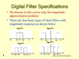
Professor A G Constantinides
1
Digital Filter Specifications
• We discuss in this course only the magnitude
approximation problem
• There are four basic types of ideal filters with
magnitude responses as shown below

2
• These filters are unealizable because their
impulse responses infinitely long non-
causal
• In practice the magnitude response
specifications of a digital filter in the
passband and in the stopband are given with
some acceptable tolerances
• In addition, a transition band is specified
between the passband and stopband

3
• For example the magnitude response
of a digital lowpass filter may be given as
indicated below
)
( 
j
e
G

4
• In the passband we require that
with a deviation
• In the stopband we require that
with a deviation
1
)
( 

j
e
G
0
)
( 

j
e
G s

p


p

 

0


 

s
p
p
j
p e
G 


 




 ,
1
)
(
1







 s
s
j
e
G ,
)
(

5
Filter specification parameters
• - passband edge frequency
• - stopband edge frequency
• - peak ripple value in the passband
• - peak ripple value in the stopband
p

s

s

p


6
• Practical specifications are often given in
terms of loss function (in dB)
•
• Peak passband ripple
dB
• Minimum stopband attenuation
dB
)
(
log
20
)
( 10

 j
e
G


G
)
1
(
log
20 10 p
p 
 


)
(
log
20 10 s
s 
 


7
• In practice, passband edge frequency
and stopband edge frequency are
specified in Hz
• For digital filter design, normalized
bandedge frequencies need to be computed
from specifications in Hz using
T
F
F
F
F
p
T
p
T
p
p 

 2
2




T
F
F
F
F
s
T
s
T
s
s 

 2
2




s
F
p
F

8
• Example - Let kHz, kHz, and
kHz
• Then
7

p
F 3

s
F
25

T
F


 56
.
0
10
25
)
10
7
(
2
3
3




p


 24
.
0
10
25
)
10
3
(
2
3
3




s

9
• The transfer function H(z) meeting the
specifications must be a causal transfer
function
• For IIR real digital filter the transfer
function is a real rational function of
• H(z) must be stable and of lowest order N
for reduced computational complexity
Selection of Filter Type
1

z
N
N
M
M
z
d
z
d
z
d
d
z
p
z
p
z
p
p
z
H 
















2
2
1
1
0
2
2
1
1
0
)
(

10
• For FIR real digital filter the transfer
function is a polynomial in with real
coefficients
• For reduced computational complexity,
degree N of H(z) must be as small as
possible
• If a linear phase is desired, the filter
coefficients must satisfy the constraint:




N
n
n
z
n
h
z
H
0
]
[
)
(
]
[
]
[ n
N
h
n
h 


1

z

11
• Advantages in using an FIR filter -
(1) Can be designed with exact linear phase,
(2) Filter structure always stable with
quantised coefficients
• Disadvantages in using an FIR filter - Order
of an FIR filter, in most cases, is
considerably higher than the order of an
equivalent IIR filter meeting the same
specifications, and FIR filter has thus higher
computational complexity

12
FIR Design
FIR Digital Filter Design
Three commonly used approaches to FIR
filter design -
(1) Windowed Fourier series approach
(2) Frequency sampling approach
(3) Computer-based optimization methods

13
Finite Impulse Response
Filters
• The transfer function is given by
• The length of Impulse Response is N
• All poles are at .
• Zeros can be placed anywhere on the z-
plane





1
0
).
(
)
(
N
n
n
z
n
h
z
H
0

z

14
FIR: Linear phase
• Linear Phase: The impulse response is
required to be
• so that for N even:
)
1
(
)
( n
N
h
n
h 













1
2
1
2
0
).
(
).
(
)
(
N
N
n
n
N
n
n
z
n
h
z
n
h
z
H
 












1
2
0
)
1
(
1
2
0
).
1
(
).
(
N
n
n
N
N
n
n
z
n
N
h
z
n
h
 
 




1
2
)
(
N
m
n
z
z
n
h N
m 

15
FIR: Linear phase
• for N odd:
• I) On we have for N even, and
+ve sign
 
 




 











 



1
2
1
0
2
1
2
1
).
(
)
(
N
n
N
m
n
z
N
h
z
z
n
h
z
H
1
: 
z
C
 










 









 
 1
2
0
2
1
2
1
cos
).
(
2
.
)
(
N
n
N
T
j
T
j N
n
T
n
h
e
e
H 



16
FIR: Linear phase
• II) While for –ve sign
• [Note: antisymmetric case adds rads to
phase, with discontinuity at ]
• III) For N odd with +ve sign
 










 









 
 1
2
0
2
1
2
1
sin
).
(
2
.
)
(
N
n
N
T
j
T
j N
n
T
n
h
j
e
e
H 


2
/

0










 






 

2
1
)
( 2
1
N
h
e
e
H
N
T
j
T
j







 










 




2
3
0 2
1
cos
).
(
2
N
n
N
n
T
n
h 

17
FIR: Linear phase
• IV) While with a –ve sign
• [Notice that for the antisymmetric case to
have linear phase we require
The phase discontinuity is as for N even]










 










 









 
 2
3
0
2
1
2
1
sin
).
(
.
2
)
(
N
n
N
T
j
T
j N
n
T
n
h
j
e
e
H 


.
0
2
1






 
N
h

18
FIR: Linear phase
• The cases most commonly used in filter
design are (I) and (III), for which the
amplitude characteristic can be written as a
polynomial in
2
cos
T


19
FIR: Linear phase
For phase linearity the FIR transfer
function must have zeros outside the
unit circle

20
FIR: Linear phase
• To develop expression for phase response
set transfer function
• In factored form
• Where , is real &
zeros occur in conjugates
n
nz
h
z
h
z
h
h
z
H 






 ...
)
( 2
2
1
1
0
)
1
(
).
1
(
)
( 1
2
1
1
1
1




 
 
 z
z
K
z
H i
n
i
i
n
i


1
,
1 
 i
i 
 K

21
FIR: Linear phase
• Let
where
• Thus
)
(
)
(
)
( 2
1 z
N
z
KN
z
H 
)
1
ln(
)
1
ln(
)
ln(
))
(
ln(
2
1
1
1
1
1
 

 






n
i
i
n
i
i z
z
K
z
H 

)
1
(
)
( 1
1
1
1


 
 z
z
N i
n
i
 )
1
(
)
( 1
2
1
2


 
 z
z
N i
n
i


22
FIR: Linear phase
• Expand in a Laurent Series convergent
within the unit circle
• To do so modify the second sum as
)
1
1
ln(
)
ln(
)
1
ln(
2
1
1
2
1
1
2
1
z
z
z
i
n
i
i
n
i
i
n
i 

  

 

 






23
FIR: Linear phase
• So that
• Thus
• where
)
1
1
ln(
)
1
ln(
)
ln(
)
ln(
))
(
ln(
2
1
1
1
1
2  

 






n
i i
n
i
i z
z
z
n
K
z
H


m
N
m
m
m
N
m
z
m
s
z
m
s
z
n
K
z
H
2
1
1
2 )
ln(
)
ln(
))
(
ln( 



 






1
1
1
n
i
m
i
N
m
s  




1
1
2
n
i
m
i
N
m
s 

24
FIR: Linear phase
• are the root moments of the minimum
phase component
• are the inverse root moments of the
maximum phase component
• Now on the unit circle we have
and

j
e
z 
)
(
)
(
)
( 


 j
j
e
A
e
H 
1
N
m
s
2
N
m
s

25
Fundamental Relationships
• hence (note Fourier form)



 jm
N
m
m
jm
N
m
j
e
m
s
e
m
s
jn
K
e
H
2
1
1
2
)
ln(
))
(
ln( 



 



)
(
))
(
ln(
)
)
(
ln(
))
(
ln( )
(



 


j
A
e
A
e
H j
j




 m
m
s
m
s
K
A
N
m
m
N
m
cos
)
(
)
ln(
))
(
ln(
2
1
1



 





 m
m
s
m
s
n
N
m
m
N
m
sin
)
(
)
(
2
1
1
2



 




26
FIR: Linear phase
• Thus for linear phase the second term in the
fundamental phase relationship must be identically
zero for all index values.
• Hence
• 1) the maximum phase factor has zeros which are
the inverses of the those of the minimum phase
factor
• 2) the phase response is linear with group delay
equal to the number of zeros outside the unit circle

27
FIR: Linear phase
• It follows that zeros of linear phase FIR
trasfer functions not on the circumference
of the unit circle occur in the form
 1

 i
j
ie 


28
Design of FIR filters: Windows
(i) Start with ideal infinite duration
(ii) Truncate to finite length. (This produces
unwanted ripples increasing in height near
discontinuity.)
(iii) Modify to
Weight w(n) is the window
 
)
(n
h
)
(
).
(
)
(
~
n
w
n
h
n
h 

29
Windows
Commonly used windows
• Rectangular 1
• Bartlett
• Hann
• Hamming
•
• Blackman
•
• Kaiser
2
1


N
n
N
n
2
1







N
n

2
cos
1







N
n

2
cos
46
.
0
54
.
0














N
n
N
n 
 4
cos
08
.
0
2
cos
5
.
0
42
.
0
)
(
1
2
1 0
2
0 
 J
N
n
J

















30
Kaiser window
• Kaiser window
β Transition
width (Hz)
Min. stop
attn dB
2.12 1.5/N 30
4.54 2.9/N 50
6.76 4.3/N 70
8.96 5.7/N 90

31
Example
• Lowpass filter of length 51 and 2
/

 
c
0 0.2 0.4 0.6 0.8 1
-100
-50
0
/
Gain,
dB
Lowpass Filter Designed Using Hann window
0 0.2 0.4 0.6 0.8 1
-100
-50
0
/
Gain,
dB
Lowpass Filter Designed Using Hamming window
0 0.2 0.4 0.6 0.8 1
-100
-50
0
/
Gain,
dB
Lowpass Filter Designed Using Blackman window

32
Frequency Sampling Method
• In this approach we are given and
need to find
• This is an interpolation problem and the
solution is given in the DFT part of the
course
• It has similar problems to the windowing
approach
2
/

 
c





 

1
0 1
2
.
1
1
).
(
1
)
(
N
k k
N
j
N
z
e
z
k
H
N
z
H 
)
(k
H
)
(z
H

33
Linear-Phase FIR Filter
Design by Optimisation
• Amplitude response for all 4 types of linear-
phase FIR filters can be expressed as
where
)
(
)
(
)
( 

 A
Q
H 









4
Type
for
),
2
/
sin(
3
Type
for
),
sin(
2
Type
for
/2),
cos(
1
Type
for
,
1
)
(




Q

34
• Modified form of weighted error function
where
)]
(
)
(
)
(
)[
(
)
( 



 D
A
Q
W 

E
]
)
(
)[
(
)
( )
(
)
(




 Q
D
A
Q
W 

)]
(
~
)
(
)[
(
~


 D
A
W 

)
(
)
(
)
(
~


 Q
W
W 
)
(
/
)
(
)
(
~


 Q
D
D 

35
• Optimisation Problem - Determine
which minimise the peak absolute value
of
over the specified frequency bands
• After has been determined, construct
the original and hence h[n]
)]
(
~
)
cos(
]
[
~
)[
(
~
)
(
0



 D
k
k
a
W
L
k




E
]
[
~ k
a
R


)
( 
j
e
A
]
[
~ k
a

36
Solution is obtained via the Alternation
Theorem
The optimal solution has equiripple behaviour
consistent with the total number of available
parameters.
Parks and McClellan used the Remez
algorithm to develop a procedure for
designing linear FIR digital filters.

37
FIR Digital Filter Order
Estimation
Kaiser’s Formula:
• ie N is inversely proportional to transition
band width and not on transition band
location





2
/
)
(
6
.
14
)
(
log
20 10
p
s
s
p
N




38
Estimation
• Hermann-Rabiner-Chan’s Formula:
where
with










2
/
)
(
]
2
/
)
)[(
,
(
)
,
( 2
p
s
p
s
s
p
s
p F
D
N



 
s
p
p
s
p a
a
a
D 



 10
3
10
2
2
10
1 log
]
)
(log
)
(log
[
)
,
( 



]
)
(log
)
(log
[ 6
10
5
2
10
4 a
a
a p
p 

 

]
log
[log
)
,
( 10
10
2
1 s
p
s
p b
b
F 


 


4761
.
0
,
07114
.
0
,
005309
.
0 3
2
1 


 a
a
a
4278
.
0
,
5941
.
0
,
00266
.
0 6
5
4 

 a
a
a
51244
.
0
,
01217
.
11 2
1 
 b
b

39
Estimation
• Fred Harris’ guide:
where A is the attenuation in dB
• Then add about 10% to it


 2
/
)
(
20 p
s
A
N



40
Estimation
• Formula valid for
• For , formula to be used is obtained
by interchanging and
• Both formulae provide only an estimate of
the required filter order N
• If specifications are not met, increase filter
order until they are met
s
p 
 
s
p 
 
p
 s


6-Digital filters (FIR).ppt

Recommended

Recommended

More Related Content

Similar to 6-Digital filters (FIR).ppt

Similar to 6-Digital filters (FIR).ppt (20)

Recently uploaded

Recently uploaded (20)

6-Digital filters (FIR).ppt