its about aquity premimums

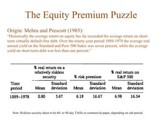
1. The Equity Premium Puzzle
Origin: Mehra and Prescott (1985):
“Historically the average return on equity has far exceeded the average return on short-
term virtually default-free debt. Over the ninety-year period 1889-1978 the average real
annual yield on the Standard and Poor 500 Index was seven percent, while the average
yield on short-term debt was less than one percent.”
Note: Riskless security taken to be 60- to 90-day T-bills or commercial paper, depending on sub-period

2. The Equity Premium Puzzle
Follow-on studies:
Siegel (1991, 1992) – Extends the period back to 1802. Over 1802-1870, 1871-
1925, and 1926- 1990, real compound equity returns were 5.7, 6.6, and 6.4
percent, respectively. However, returns on short-term government bonds have
fallen dramatically, the figures for the same three time periods being 5.1, 3.1,
and 0.5 percent. Thus, there was no equity premium in the first two-thirds of the
nineteenth century (because bond returns were high), but over the last 120
years, stocks have had a significant edge.

3. The Equity Premium Puzzle
Follow-on studies:
Siegel and Thaler (1997)
“Suppose your great grandmother had some money lying around at the end of
1925 and, with rational expectations, anticipated your birth and decided to
bequeath you $1000. Naturally, since you weren't born yet, she invested the
money, and being worried about the speculative boom in stocks going on at the
time, she put the money in Treasury bills, where it remained until December 31,
1995. On that date it was worth $12,720.
Imagine, instead that she had invested the money in a (value-weighted) portfolio
of stocks. You would now have $842,000, or 66 times as much money.“

4. The Equity Premium Puzzle
Follow-on studies:
Ilmanen (2011) – Sample includes post-2000 weak period for equities.

5. The Equity Premium Puzzle
Why is a risk premium of 6.2% per year “too much”?
Mehra and Prescott (1985) use a consumption-based asset pricing model and examine the
equity premia it generates when it is fed the sample statistics regarding consumption
growth, consumption growth’s sample correlation with stock returns and a range of
parameter values for people’s willingness to substitute consumption between successive
yearly time periods. The highest equity premium that they were able to generate was 0.35%
per year.
0.35%

6. The Equity Premium Puzzle
Why is a risk premium of 6.2% per year “too much”? (continued)
Another way of looking at the Mehra and Prescott result is in terms of the coefficient of risk
aversion that the historical consumption and excess return data imply, given the utility
functions that they employ.
Recall that an investor’s coefficient of relative risk aversion is an important factor in
determining how much extra expected return he or she requires from a risky investment
over the risk-free investment.
Requiring a 6.2% extra average return for stocks over the riskless investment, given an
annual standard deviation of returns for stocks of 16.5% implies a relative risk aversion
coefficient for the representative investor of more than 30.
So just how high a risk aversion coefficient is 30?

7. The Equity Premium Puzzle
A person who has a starting wealth of zero, having the utility function posited by Mehra and
Prescott and a coefficient of relative risk aversion of 30, would, when faced with an
uncertain gain that involves
-A payout of $50,000 with 50% probability
-A payout of $100,000 with 50% probability
and the choice of receiving $51,209 for certain, would select the certain sum over the
uncertain game!
Starting with a wealth level of $500K, the payout at which the same individual would prefer
the certain outcome would be $61,808. A more reasonable amount, but still seems too low.
Few people can be this afraid of risk.

8. The Equity Premium Puzzle
Follow-on studies:
Benartzi and Thaler (1995): People exhibit “myopic loss aversion”. That is, instead of
evaluating the aggregate results from risky investments over a long horizon, they evaluate
them over shorter horizons over which they are roughly doubly as sensitive to losses as
they are to gains.
This tendency to take problems one at a time has variously been labelled decision
isolation, narrow framing, narrow bracketing, or myopic loss aversion.
If investors focus on the long-term returns of stocks they would recognize how little risk
there is, relative to bonds, and would be happy to hold stocks at a smaller equity premium.
Instead, they consider short-term volatility, with frequent mental accounting losses, and
demand a substantial equity premium as compensation.

9. The Equity Premium Puzzle
Instead of a utility of wealth function, Benartzi and Thaler use a value function to evaluate
individual investment opportunities. This is the same value function put forth by
Kahneman and Tversky in their papers on prospect theory (1979, 1992):
where:
x = return
λ is a coefficient capturing investor’s degree of loss-aversion
α and β capture risk-aversion in the domain of gains and losses, respectively.
λ = 2.25; α = β = 0.88 (These are estimates by Kahneman and Tversky)

10. The Equity Premium Puzzle
Prospective Utility
where pi is the decision weight (derived from its estimated probability) of outcome xi.
This is the analogue of expected utility from classical microeconomic theory.

11. The Equity Premium Puzzle
Mental accounting, evaluation period and myopia
• Mental accounting refers to the implicit methods used by investors to code and evaluate
financial outcomes.
• One aspect of mental accounting that is crucial in this context is the evaluation period.
• Evaluation period is the length of time over which an investor aggregates returns.
• In the presence of loss aversion, aggregation rules are not neutral! The following example
illustrates this:
Consider following bet:
{$200, .5; -$100, .5}
Is this an attractive gamble?
With loss aversion, expected value from the bet would be (assuming decision weights =
probabilities, a = b = 1 for simplicity):
“Prospective” utility of the gamble = (0.5)(200) + (2.25)(0.5)(-100) = -12.5

12. The Equity Premium Puzzle
Mental accounting, evaluation period and myopia (continued)
•Now, assume you have two chances at the same bet: the distribution of outcomes created by the
portfolio of two bets would be:
{$400, .25; 100, .50; -$200, .25}
Prospective Utility = (0.25)(400) + (0.5)(100) + (2.25)(0.25)(-200) = +37.5
This yields positive prospective utility!
Though simple repetitions of the single bet are unattractive if evaluated one at a time. e.g. for two
bets: a value of 2 x (-12.5) = -25
As this example illustrates, when decision-makers are loss averse, they will be more willing to
take risks if they evaluate their performance (or have their performance evaluated) infrequently.
• BT thus suggests that the evaluation horizon matters how investors experience risk
psychologically.

13. The Equity Premium Puzzle
Mental accounting, evaluation period and myopia (continued)
• The evaluation period should not be confused with the planning horizon of the investor. A
young investor, for example, might be saving for retirement 30 years off in the future, but
nevertheless experience the utility associated with the gains and losses of his investment
every quarter when he opens a letter from his mutual fund. In this case his horizon is 30
years but his evaluation period is 3 months. In terms of the Benartzi Thaler model an
investor with an evaluation period of one year behaves very much as if he had a planning
horizon of one year.
• Myopic investors have short evaluation horizons. They experience risk by focusing on a
series of short-term movements. In doing so, they frame their decisions in a way that
maximises the impact of loss aversion.
• Myopic loss aversion: The combination of short evaluation horizon and loss aversion.

14. The Equity Premium Puzzle
Mental accounting, evaluation period and myopia (continued)
• Questions:
If investors have prospect theory preferences, how often would they have to evaluate their
portfolios to explain the equity premium?
Benartzi and Thaler pose the question two ways. First, what evaluation period would make
investors indifferent between holding all their assets in stocks or bonds? Second, for an
investor with this evaluation period, what combination of stocks and bonds would
maximize prospective utility?
• Their methodology:
- They use simulations to answer both questions.
- They use monthly returns data for bonds, stocks and treasury bills from 1926-1990.
- They simulate distributions of returns over different horizons (from 1 month and up) by
selecting months at random from history.
- They then calculate prospective utility of each asset for the different time horizons.

15. The Equity Premium Puzzle
Mental accounting, evaluation period and myopia (continued)
Investor with an evaluation period of roughly 13
months indifferent between stocks and bonds

16. The Equity Premium Puzzle
Mental accounting, evaluation period and myopia (continued)
• How should these results be interpreted? Is the 1-year evaluation period plausible?
• Individual investors file tax returns annually.
• They receive their most comprehensive reports from their brokers, mutual funds and
retirement accounts once a year.
• Institutional investors take annual reports most seriously.
• Fund managers are also evaluated frequently, reducing their evaluation period below that
of their clients (especially pension funds). Agency problems and short horizons/investment
goals.

17. The Equity Premium Puzzle
Mental accounting, evaluation period and myopia (continued)
• Answer to the second question:

18. The Equity Premium Puzzle
Mental accounting, evaluation period and myopia (continued)

19. The Equity Premium Puzzle
Mental accounting, evaluation period and myopia (continued)
• One weakness of the Benartzi - Thaler approach:
- investors get no utility at all from consumption
• Challenge: build a model in which investors get utility from both consumption and
narrowly framed components of wealth
• To address the equity premium properly, need to introduce consumption in a non-
trivial way
– preferences must include “utility of consumption” term alongside the prospect
theory term
– Barberis, Huang, and Santos (QJE, 2001) have this in mind in their model.

20. The Equity Premium Puzzle
Barberis, Huang, Santos (2001) approach:
• “Consistent with prospect theory, the investor in our model derives utility not only
from consumption levels but also from changes in the value of his financial wealth. “
• “He is much more sensitive to reductions in wealth than to increases, the loss-aversion
feature of prospective utility. “
• “Moreover, consistent with experimental evidence, the utility he receives from gains
and losses in wealth depends on his prior investment outcomes; prior gains cushion
subsequent losses, the so-called “house-money effect” while prior losses intensify the
pain of subsequent shortfalls. “
• The inclusion of a house-money effect, i.e., the idea that loss aversion varies
dynamically with prior gains and losses, allows Barberis, Huang and Santos to generate
a risk premium for stocks close to historical averages. Their model thus implies that
investors become more conservative in down markets.

21. The Equity Premium Puzzle
Three important points by Mehra (2011) on the Puzzle:
1) The risk-free asset for a typical investor is not T-bills:
If one uses longer-term maturity Treasury securities such as TIPS or mortgage-backed
securities backed by housing agencies (GNMA, etc.) the premium narrows by roughly 2
percent!

22. The Equity Premium Puzzle
Three important points by Mehra (2011) on the Puzzle:
2) The marginal investor is likely to be a borrower, not a lender.
• Think of a household with a mortgage balance. Its opportunity cost when judging
investing a marginal dollar of savings into stocks is the rate on its mortgage loan, which
is on average 2% higher than the lending rate that the household is faced with.
So points 1 and 2 combined narrow the equity premium by close to 4%!

23. The Equity Premium Puzzle
Three important points by Mehra (2011) on the Puzzle:
3) The premium should depend on the life cycle stage of the marginal investor.
• Young people looking forward at the start of their lives have uncertain future wage
and equity income; furthermore, the correlation of equity income with consumption will
not be particularly high as long as stock and wage income are not highly correlated.
This is empirically the case, as documented by Davis and Willen (2000). Equity will,
therefore, be a hedge against fluctuations in wages and a “desirable” asset to hold as far
as the young are concerned.
• For the middle-aged, wage uncertainty has largely been resolved. Their future
retirement wage income is either zero or deterministic, and the innovations
(fluctuations) in their consumption occur from fluctuations in equity income. At this
stage of the life cycle, equity income is highly correlated with consumption.
Consumption is high when equity income is high, and equity is no longer a hedge
against fluctuations in consumption; hence, for this group, equity requires a
higher rate of return.

24. The Equity Premium Puzzle
Three important points by Mehra (2011) on the Puzzle:
3) The premium should depend on the life cycle stage of the marginal investor.
(continued)
• The characteristics of equity as an asset, therefore, change depending on
the predominant holder of the equity. Life-cycle considerations thus become
crucial for asset pricing. If equity is a desirable asset for the marginal investor
in the economy, then the observed equity premium will be low relative to an
economy where the marginal investor finds it unattractive to hold equity. The
deus ex machina is the stage in the life cycle of the marginal investor.
• If young people, who should find equity attractive, are subject to constraints on
borrowing against their future wage income, then the marginal investor in equity is
likely to be the older investors who will demand a higher premium from equity.

25. The Equity Premium Puzzle
Additional points brought up by researchers, as summarized by Ilmanen (2011):