Digital-communication.pdf

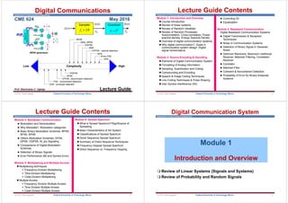
Department of Communications Engineering
Digital Communications
CME 624 May 2016
Lecture Guide
Prof. Okechukwu C. Ugweje
Complexity High
APK
M-ary PSK
QPR
CPFSK - optimal detection
MSK
OQPSK
QAM, QPSK
BPSK
Low
OOK - envelope detection
DQPSK
DPSK
CPFSK -discriminator detection
FSK - noncoherent detection
Sampler
f B
s  2
Quantizer
L k
 2
x n
( )
xk 
xk
( )
x n
x t
( )
© Prof. Okey Ugweje 1
Federal University of Technology, Minna
Lecture Guide Contents
Module 1: Introduction and Overview
 Course Introduction
 Review of linear systems
 Review of Random Variables
 Review of Random Processes:
Autocorrelation, Cross-correlation, Power
spectral density, Energy Spectral Density
 Overview of digital communication systems
 Why digital communication?, Goals in
communication system design, Digital
signal nomenclature
Module 2: Source Encoding & Decoding
 Elements of Digital Communication System
 Formatting of Analog Information
 Sampling, Quantization and Coding
 Compounding and Encoding
 Speech & Image Coding Techniques
 Line Coding Techniques & Pulse Shaping
 Inter Symbol Interference (ISI)
 Controling ISI
 Equalization
Module 3: Baseband Communication
Digital Baseband Communication Systems
 Digital Transmission & Reception
Techniques
 Noise in Communication Systems
 Detection of Binary Signal in Gaussian
Noise
 Optimum Receivers: Maximum Likelihood
Receiver, Matched Filtering, Correlation
Receiver
 Correlator
 Matched Filter
 Coherent & Noncoherent Detection
 Probability of Error for Binary Antipodal
Systems
Lecture Guide Contents
Module 4: Bandpass Communication
 Modulation and Demodulation
 Why Modulate?, Modulation categories
 Basic Binary Modulation Schemes: BPSK,
BFSK, BPSK
 Others Modulation Schemes: DPSK,
QPSK, OQPSK, M_ary Signaling
 Comparisons of Digital Modulation
Schemes
 Detection of Binary Signals
 Error Performance (Bit and Symbol Error)
Module 5: Multiplexing and Multiple Access
 Multiplexing techniques
 Frequency-Division Multiplexing
 Time-Division Multiplexing
 Code-Division Multiplexing
 Multiple Access
 Frequency Division Multiple Access
 Time Division Multiple Access
 Code Division Multiple Access
Module 6: Spread Spectrum
 What is Spread Spectrum?/Significance of
Spreading
 Basic Characteristics of SS System
 Classifications of Spread Spectrum
 Direct Sequence Spread Spectrum
 Summary of Direct Sequence Techniques
 Frequency Hopped Spread Spectrum
 Direct Sequence vs. Frequency Hopping
Digital Communication System
Module 1
Introduction and Overview
 Review of Linear Systems (Signals and Systems)
 Review of Probability and Random Signals

 Introductions
 Course Outline/Syllabus
 Course Calendar
 Course Overview
Introduction and Handout
 Note:
 Some of the material contained in Module 1 is a review
of prerequisite materials covered in undergraduate
classes such as:
 Signals and Systems
 Communications and Signal Processing
 Random Signals and Processes
 Some of the materials are included in this section for
your benefit
 It is your responsibility to review most of the material in
this Module
 Most materials in this section can be found in Chapter
1 and the Appendix of the recommended textbook
 Signals and Systems
 Continuous Convolution
 Parseval’s’ theorem
 Linear Transform
 Fourier Transform Techniques
 Concept of Bandwidth/ Filtering
Signals and Systems
Signals - 1
Signals are used to convey information
Signals and waveforms (voltage, current and intensity)
are central to communication and signal processing
Signals can be viewed either in time or frequency
domain
A signal is any physical quantity that varies with time,
space, or any other independent variables
Often, the independent variables for most signals is
“time”
Theoretical signals can be described mathematically,
graphically or in tabular form
Real signals are however difficult to describe, and more
often can be described approximately

Signals - 2
Mathematically, a signal is defined as a function of one
or more independent variables, e.g.,
x(t) = 10t
x(t) = 5t2
s(x,y) = 3x + 2xy + 10y2
Sometimes the functional dependence on the
independent variable is not precisely known, e.g.,
speech signal
Sometimes a signal is a combination of other signals
e.g., sum of sinusoid of different amplitudes,
frequency & phase
 
1
( ) ( )sin 2 ( ) ( )
n
i i i
i
s t A t F t t
 

 

Signals - 3
Mathematically, a signal is defined as a function of one or
more independent variables, e.g.,
 x(t) = 10t
 x(t) = 5t2
 s(x,y) = 3x + 2xy + 10y2
Sometimes the functional dependence on the independent
variable is not precisely known, e.g., speech signal
Sometimes a signal is a combination of other signals
 e.g., sum of sinusoid of different amplitudes, frequency & phase
Signals are the inputs outputs, and internal functions that
the systems process or produce, such as voltage,
current, pressure, displacements, intensity, etc.
 
1
( ) ( )sin 2 ( ) ( )
n
i i i
i
s t A t F t t
 

 

Signals - 4
The variable time may be continuous or discrete and the
value of the signal may be represented as
 Continuous-valued x(t)
 Discrete-valued x(nts)
 Quantized xQ(t), and
 Digital x[n]
These types of signals occur at different stages of the
process
Other variables (distance, angle, etc.) can also be the
independent variable, especially for 2-D signals like
images and video
Physical realizable signals must
 Have time duration
 Occupy finite frequency spectrum
 Are continuous (as in analog signal)
 Have finite peak value, and
 Are real-valued
All real-world signals will have these properties
Sometimes we use mathematical signal models which violate
these conditions
 e.g., Dirac delta function (or impulse function)
The most commonly used analog signals are the sinusoidal
signals (sine, cosine, etc.)
In communication systems, we are concerned with info
bearing signals that evolve as a function of the independent
variable, t
Signals - 5

Systems - 1
When signals are corrupted by noise, they no longer convey
the required information directly, hence they often require
processing
 Radio receivers are especially sensitive to noise
Signals are processed by systems, which may modify them
or extract additional information from them
Thus, a system is an entity that processes a set of signals
(inputs) to yield another set of signals (outputs)
A system can also be associated to the signal as in the
source or sink of the signal
A system may be made up of physical components
(hardware realization), as in electrical, mechanical, or
hydraulic systems, or it may be an algorithm (software
realization) that computes an output from an input signal
Systems - 2
 Many systems have signals that are not wanted (commonly
known as noise or interference)
 A system is a device, process, or algorithm that, given an
input x(t), produces an output y(t)
 A system is characterized by its input (excitation or forcing
function), its output (response), and the rules of operation
(internal functions)
 From a communication engineers’ viewpoint, a system is a law
that assigns output signals to various input signals
 Systems may be realized as an integration of sub-systems or
as a single entity
 In practice, systems with feedback is of great importance
Systems - 3
Systems may be classified functionally as in
Analyzers, Synthesizers, Transducers, Channels,
Filters, and Equalizers, etc.
or descriptively as in
linear, nonlinear, causal, discrete, continues, time
invariant, etc.
Examples of Systems
Electronic systems: resistors, inductors, Radio/TV,
phone networks, sonar and radar, guidance &
navigation, satellite, lab instrumentation, biomedical
instrumentation, etc.
Mechanical systems: loudspeakers, microphones,
vibration analyzers, springs, dampers
Systems - 4
To understand the behavior of systems
(electronic/mechanical), the response to inputs
(usually signals) must be understood
Terminology of Systems
State:
Variables that allow us to determine the energy level
of the system
All physical systems are referenced to zero-energy
state, e.g., ground state, rest state, relaxed state
Initial Conditions
The initial conditions or initial state is the state of the
system before an input is applied

Broad Classification of Systems
 We are
interested only
on the systems
that intersect the
dotted path.
Distributed
Parameters
SYSTEMS
Lumped Parameters
Stochastic Deterministic
Continuous Time Discrete Time
Nonlinear Linear
Nonlinear Linear
Time
Varying
Time
Invariant
Time
Varying
Time
Invariant
Systems - 5 Department of Communications Engineering
Operation on Linear Systems
 An operator, T, is a rule to transform one function to another
 Additive
 Homogeneous
 Principle of Superposition
 Superposition implies both additive & homogeneous rules
 If a system fails either rule, the function is nonlinear
 Addition or homogeneity is sufficient condition to test for
linearity
T x t y t
( ) ( )
  
T x t x t T x t T x t
1 2 1 2
( ) ( ) ( ) ( )
  
k p k p k p
T Kx t KT x t
( ) ( )
    
T Ax t Bx t AT x t BT x t
1 2 1 2
( ) ( ) ( ) ( )
  
k p k p k p
Systems - 6
Linear Time-Invariant (LTI) Systems
Linear systems are characterized by the ability to accept
input and produce output in response to the input
Most communication systems can be modeled as linear
systems with signals forming the input and output functions
h(t)
h[n]
H(ejw)
H(f)
H(z)
LTI
y(t)
y[n]
Y(ejw)
Y(f)
Y(z)
x(t)
x[n]
x(ejw)
X(f)
X(z)
Time Function
Pole-Zero Plot
Difference Equation
H - Function
Frequency Function
Why study signals and systems?
In signals and systems theory we study the definition
and description of signals, and the behavior of systems
under different conditions
Signals form the inputs, outputs and internal
functions of systems
In electrical & computer engineering, the understanding
of signals and the behavior of systems is of immense
importance
Communication engineers are concerned with systems
which transmit, receive, and process signals carrying
information
Hence before one can characterize a system, one must
be able to characterize the system

Size of a Signal - 1
 The size of a signal is the value of the strength of the
signal
 The signal strength may be measures in its entirety
or in a given interval
 Such a measure must consider not only the signal
amplitude, but also its duration
 There are two major ways of determining the signal
strength
1. Signal Energy
 A signal is classified as energy-type if its energy Eg is
finite (0<Eg<)
 Energy may be computed in either time or frequency
domain, whichever is easier using the following
formula
 where G(f) is the Fourier transform of g(t)
 All time-limited signals of finite amplitude are energy
signals
 Energy signals have zero power
 Since signal energy also depends on the “load” the actual
signal energy should be normalized by the load R
2 2 2
/2
lim
/2
( ) ( ) ( )
T
g T
T
E g t dt g t dt G f df
 
  

  
   (unit)2s
2. Signal Power
 A signal is power-type if its power Pg is finite (0<Pg<)
 The power Pg of a signal can be computed using the
formula
 Notice that the signal power is the time-average
(mean) of the signal amplitude squared
 Most periodic signals are power-type signals
 For periodic signals Eg & Pg can be computed by
integrating over one period
/ 2
lim lim
/ 2
2 2
1 1
2 ( ) ( )
T T
T T
T T
g T T
P g t dt g t dt
 
 

 
 (unit)2
Important Signal Classifications
Deterministic and Random Signals
 Value of the signal is known or not known at all
times
Periodic and Non-periodic Signals
Analog (Continuous-Time) and Discrete Signals
 Exists for all times t vs. exists at discrete time
only
Signals and Spectra - 1
0
( ) ( ),
x t x t T t
      

 Energy- and Power-Type Signals
with waveform
 Unit Impulse Function
.5 2 2
.5
lim ( ) ( )
T
X T
T
E x t dt x t dt

 

 
 
.5 2 2
.5
1 1
lim ( ) ( )
T
x T
T T T
P x t dt x t dt

 

 
 
( ) 1, ( ) 0 0
t dt t for t
 


  

0
( ) ( ) ( )
o
x t t d x t
  


 

.5 2
.5
( )
T
T
x T
E x t dt

 
.5 2
.5
1 1
( )
T
T T
x x T
T T
P E x t dt

  
 Others
 Even and Odd Signals
 Real and Complex Signals
 Causal and Noncausal
Spectral Density
 Energy Spectral Density
 Power Spectral Density
 For periodic signals, the PSD is given by
2
2
( )
2
0
( ) '
( )
( ) ( ) is defined as energy spectral density
( )
X
X
f
X
X
E x t dt df Parseval s Theorem
x f
f df f
f df

 

 
 



  
 
 

 



2
2
2
2
1
( )
T
T
X n
n
P x t dt power
C
T




  

 
2
0
( )
X n
n
G f C f nf




 
Examples
1. Example 1
 Signal Power
2. Example 2
 Signal Energy
3. Example 3
 Signal Energy

 Some Important or Common Signals & Functions
 Sinusoidal Signal
 Complex Exponential (harmonics)
 Unit Step Function [denoted by u(t)]
 Ramp Function [denoted by r(t)]
 Rectangular Pulse Function [denoted by rect(t) or
(t)]
 Triangular Pulse Function[denoted by (t)]
 Sign (Signum) Function [denoted by sgn(t)]
 Sinc Function [denoted by sinc(t)]
 Impulse (Delta, Dirac) Function [denoted by (t)]
 Operations on Signals
 Amplitude Scaling
 Amplitude Shifting
 Time Shifting
 Displaces a signal in time without changing its
shape
( ) ( )
"+"shifts the signal left by
"-" shifts the signal right by (delayed)
y t x t 


 
 Time Scaling
 Slows down or speeds up time which results in signal
compression or stretching
 The expression
 Reflection or Folding
 A scaling operation with  = -1  x(t) = x(-t)
 The mirror image of x(t) about the y-axis through t = 0
 Operations in Combinations
 x(t)  delay (shift right) by   x(t-)
 compress by   x(t-)
 x(t)  compress by   x(t)
 delay (shift right) by /  x(t-)
( )
t
y t x

 
  
 
 Some useful signal operations and models
 Continuous/Discrete Convolution
 Parseval’s’ theorem
 Hilbert Transform
Concept of Bandwidth and Filtering
 Some Important Properties of Signals
 DC Value
 Is the time average of a signal or the time average
over a finite interval [t1, t2]
 Average Power
 The ensemble average
 RMS Value

 Fourier Series and Transform
 Definition and Properties
 Important Fourier transform cases
 Energy and power spectral density
 Different Types of Sampling Techniques
 Idea Sampling
 Natural Sampling
 Sample-and-Hold
Examples
4. Example 4
 Periodicity of Signal
5. Example 5
 Even and Odd Signals
 Even  x(t) = x(-t)
 Odd  x(t) = -x(-t)
6. Example 6
 Even and Odd Signals
 
0
( )
g t g t T
 
Examples
7. Example 7 : Convolution
 Convolution is a technique of finding the zero state
response of LTI system
8. Example 8: Convolution
h(t) y(t)
x(t)
( ) ( ) ( ) ( ) ( ) ( ) ( )
y t x t h t x h t d x t h d
     
 
 
     
 
Fourier Transform Table

Fourier Transform Pair
Examples
9. Example 9: Fourier Transform
10.Example 10: Fourier Transform
13.Example 13: Inverse Fourier Transform
X f F x t x t e j ftdt
( ) ( ) ( )
  
z


2
x t F X f X f e j ftdf
( ) ( ) ( )
  z



1 2
 Probability Theory
 Distribution Functions
 Density Functions
 Expectations
 Random Processes, etc
Review of Probability and
Random Signals
Please review the course
CME621:Stochastic
Processes
Examples – Random Signals
14. Example 14
 Random Signals
15. Example 15
 Random Processes

Module 2
Source Encoding & Decoding
 Elements of Digital Communication
 Formatting of Analog Signal
 Sampling and Quantization
 Compounding
 Encoding and Line Coding Techniques
 Intersymbol interference
Elements of Digital
Communication System
Elements of Digital Communication - 1
 Each of these blocks represents one or more transformations
 Each block identifies a major signal processing function which changes or
transforms the signal from one signal space to another
 Some of the transformation block overlap in functions
Elements of Digital Communication - 2
Format Multiplex
Channel
Encoder
Source
Encoder
Spread
Modulate
Format Demultiplex
Channel
Decoder
Source
Decoder
Despread
Demodulate
&
Detect
Performance
Measure
Bits or
Symbol
To other
destinations
From other
sources
Digital
input
Digital
output
Source
bits
Source
bits
Channel
bits
Carrier & symbol
synchronization
Channel
bits
$
mi
n s
mi
l q
Pe
Multiple
Access
Waveforms
Multiple
Access
Tx
Rx

Why Digital Communications? - 1
1. Advantages
 Two-state signal representation
 Hardware is more flexible
 Hardware implementation is flexible and permits the use of
microprocessors, mini-processors, LSI or VLSI, etc.
 Low cost
 With LSI/VLSI, implementation cost is reduced
 Easy to regenerate the distorted signal
 Repeaters can detect a digital signal and retransmit a new,
clean (noise free) signal
 Hence, prevent accumulation of noise along the path
Less subject to distortion and interference
 Digital system is more immune to channel noise/ distortion
Easier and more efficient to multiplex several digital
signals
 Digital multiplexing techniques – TDMA and CDMA - are
easier to implement than analog techniques such as FDMA
Can combine different signal types – data, voice,
TV, text, etc.
 It is possible to combine both format for transmission
through a common medium
Can use packet switching
Encryption and privacy techniques are easier to
implement
Better overall performance
 Inherently more efficient than analog techniques in
realizing the exchange of SNR for bandwidth
2. Disadvantages
 Requires reliable “synchronization”
 Requires A/D conversions at high data rate
 Requires larger bandwidth (require BW efficient
MODEM)
 Banalog = W Hz
 Bdigital = nW Hz
– where n is the # of bits used to quantize the amplitude
of the signal
 Generally an increase in complexity over analog
system
 To maximize transmission rate, R, e.g., symbols per sec
 To minimize bit error rate, Pe, or Pb
 To minimize required power, Eb/No (or ~ly required signal
power)
 To minimize required systems bandwidth, W
 To maximize system utilization, U
 To minimize system complexity, Cx
Goals in Communication System Design
R U Pe W Cx Eb/No
• In most practical
applications trade-
offs are necessary

 Information Source
Discrete output values, e.g. Keyboard (1~26 (A~Z) symbols)
Analog signal source information is continuous valued
 Textual Message
A meaningful sequence of character or symbols, e.g.,
 How are you? I am ok, thank you; I feel like a million dollars!
 Character
 Member of an alphanumeric/symbol (A ~ Z, 0 ~ 9)
 Characters can be mapped into a sequence of binary digits
using one of the standardized codes such as
 ASCII: American Standard Code for Information
Interchange
 Others: EBCDIC, Hollerith, Baudot, Murray, Morse, etc.
Digital Signal Nomenclature - 1
Symbol
 A digital message made up of groups of k-bits considered as a unit
 A member of source alphabet. May or may not be binary, e.g. 2
symbol binary, 4 symbol PSK, 128 symbol ASCII
Digital Message
Messages constructed from a finite # of symbols (26 letters, 10
numbers, “space” and punctuation marks).
 Hence a text is a digital message with about 50 symbols
Morse-coded telegraph message is a digital message
constructed from 2 symbols “Mark” and “Space”
M_ary
A digital message constructed with M symbols
 Digital Waveform
 Current or voltage waveform that represents a digital symbol
 Binary Digit (Bit)
Fundamental unit of info made up of 2 symbols (0 and 1)
Quantity of info carried by a symbol with probability P = ½
 Bit: number with value 0 or 1
 n bits: digital representation for 0, 1, … , 2n
 Byte or Octet, n = 8
 Computer word, n = 16, 32, or 64
 n bits allows enumeration of 2n possibilities
 n-bit field in a header
 n-bit representation of a voice sample
 Message consisting of n bits
 The number of bits required to represent a message is a measure
of its information content
 More bits → More content
Binary Stream (or bit stream or baseband signal)
 A sequence of binary digits, e.g., 10011100101010
Block
 Information that occurs in
a single block
 Text message
 Data file
 JPEG image
 MPEG file
 Size = Bits / block
or bytes/block
 1 kbyte = 210 bytes
 1 Mbyte = 220 bytes
 1 Gbyte = 230 bytes
Stream
• Information that is
produced & transmitted
continuously
– Real-time voice
– Streaming video
• Bit rate = bits / second
– 1 kbps = 103 bps
– 1 Mbps = 106 bps
– 1 Gbps =109 bps

Examples of Block Information
Type Method Format Original Compressed
(Ratio)
Text Zip,
compress
ASCII Kbytes-
Mbytes
(2-6)
Fax CCITT
Group 3
A4 page
200x100
pixels/in2
256
kbytes
5-54 kbytes
(5-50)
Color
Image
JPEG 8x10 in2 photo
4002 pixels/in2
38.4
Mbytes
1-8 Mbytes
(5-30)
© Prof. Okey Ugweje Federal University of Technology, Minna 53
 L number of bits in message
 R bps speed of digital transmission system
 L/R time to transmit the information
 tprop time for signal to propagate across medium
 d distance in meters
 c speed of light (3x108 m/s in vacuum)
Use data compression to reduce L
Use higher speed modem to increase R
Place server closer to reduce d
Delay = tprop + L/R = d/c + L/R seconds
Transmission Delay
Bit Rate
 Actual rate at which info is transmitted per second
Baud Rate
 The rate at which bits are transmitted, i.e. # of signaling elements per
second
Bit Error Rate
 The probability that one bit is in error, Pb, or simply the probability of
error, Pe
Data Rate
 The rate at which info is transferred in bits per second
 If binary symbols are independent & equiprobable, the bit rate = baud
rate
Character Rate
 Characters transmitted per second
Bit Rate of Digitized Signal
Bandwidth Ws Hertz: how fast the signal changes
 Higher bandwidth → more frequent samples
 Minimum sampling rate = 2 x Ws
Representation accuracy: range of approximation error
 Higher accuracy
→ smaller spacing between approximation values
→ more bits per sample

Th e s p ee ch s i g n al l e v el v a r ie s w i th t i m(e)
Stream Information
A real-time voice signal must be digitized &
transmitted as it is produced
Analog signal level varies continuously in time
Sampling Rate and Bandwidth
A signal that varies faster needs to be sampled more
frequently
Bandwidth measures how fast a signal varies
 What is the bandwidth of a signal?
 How is bandwidth related to sampling rate?
1 ms
1 1 1 1 0 0 0 0
. . . . . .
t
x2(t)
1 0 1 0 1 0 1 0
. . . . . .
t
1 ms
x1(t)
Bandwidth of General Signals
 Not all signals are periodic
 E.g. voice signals varies according
to sound
 Vowels are periodic, “s” is noiselike
 Spectrum of long-term signal
 Averages over many sounds, many
speakers
 Involves Fourier transform
 Telephone speech: 4 kHz
 CD Audio: 22 kHz
s (noisy ) | p (air stopped) | ee (periodic) | t (stopped) | sh (noisy)
X(f)
f
0 Ws
“speech”
Analog vs. Digital Communications
Analog Digital
Older technology Newer technology
Used to design mainly for voice Used to design for data and voice
Inefficient for data Efficient for data
Noisy and error prone Noise can be easily filtered out
Lower speeds Higher speeds
High overhead Low overhead
Info is precise since recorded,
transmitted or displayed
continuously in time
Digital is accurate since info is displayed in
terms of values; but we don't know if the
precise value is displayed
Interpretation of display is harder Interpretation of display is easier
More test options
Discrete-level information
Performance measured with SNR Performance measured with BER

Analog vs. Digital Transmission
Analog transmission: all details must be reproduced accurately
Sent
Sent
Received
Received
Distortion
Attenuation
Digital transmission: only discrete levels need to be reproduced
Distortion
Attenuation
Simple Receiver:
Was original pulse
positive or
negative?
Bandwidth Dilemma
All bandwidth criteria have in common the attempt to
specify a measure of the width, W, of a nonnegative
real-valued spectral density defined for all frequencies
f < ∞
The single-sided power spectral density for a single
heterodyned pulse xc(t) takes the analytical form:
(1.73)
2
sin ( )
( )
( )
c
x
c
f f T
G f T
f f T


 

  

 
Different Bandwidth Criteria
(a) Half-power
bandwidth.
(b) Equivalent
rectangular or noise
equivalent bandwidth.
(c) Null-to-null bandwidth.
(d) Fractional power
containment
bandwidth.
(e) Bounded power
spectral density.
(f) Absolute bandwidth.
Digital Communication Transformations

Formatting of Analog
Signal
Baseband Systems
Formatting Textual Data (messages, character, symbols)
Formatting Analog Information
Sampling (see prerequisite section)
Quantization
Line Coding
Encoding and Decoding of Messages
(Baseband Systems)
Multiplex
Channel
Encoder
Spread
Modulate
Demultiplex
Channel
Decoder
Despread
Demodulate &
Detect
Bits or
Symbol
To other
destinations
From other
sources
Source bits
Source bits Channel bits
Carrier and symbol
synchronization
Channel bits

mi
l q
mi
l q

Pe
Multiple
Access
Waveforms
Multiple
Access
Format
Source
Decoder
Digital
output
Digital
input
Source
Encoder
Format
Performance
Measure
Pulse
Modulation
Digital Communication Transformations - 1
67
© Prof. Okey Ugweje Federal University of Technology, Minna
Transmit and Receive Formatting
 Transition from info source  digital symbols  info sink
Sampler Quantizer Coder
Waveform
Encoder
(Modulator)
Transmitter
Channel
Receiver
Waveform
Detector
LPF Decoder
Digital Information
Textual
Information
Analog
Information
Format
Analog
Information
Textual
Information
Digital Information
Source
Sink

Character Coding (Textual Info)
A textual info is a sequence of alphanumeric characters
Characters are encoded into bits
Groups of k bits can be combined to form new digits or
symbols of size M
A symbol set of size M is referred to as M-ary system
Textual
Message
Encoder
Group of k bits
M=2k
Waveform
Encoder
(Modulator)
... 01101 ... M_ary
2k
M 
Character coding, messages and symbols
Alphanumeric and symbolic characters are encoded
into digital bits using one of several standard formats
 ASCII
 EBCDIC
 Others Baudot, Hollerith, Morse
Example 16:
In ASCII alphabets, numbers, and symbols are encoded
using a 7-bit code
A total of 27 = 128 different characters can be
represented using a 7-bit unique ASCII code
1 0
1
0
1
1
0
1
0
1
0 0 1 1 1 0
0
0
0
0 1
7-bit ASCII
16_ary digits
(symbols)
A
U S
1 5 C
9
6 1
b7 b1
b2
b3
b4
b5
b6
b8
7-bit ASCII
Least significant
Most significant
Parity

Digital Representation of Analog Signals
Most practical signal of interest are analog in nature
e.g., speech
biological signals
seismic signals
radar signals
sonar, and
various communication signals (audio, video, text, etc)
Conversion to digital form is necessary
Interface
(A/D)
Analog
Signal
Digital
Signal
Sampling
Digitization of Analog Signals
1. Sampling: obtain samples of x(t) at uniformly spaced
time intervals
2. Quantization: map each sample into an approximation
value of finite precision
 Pulse Code Modulation: telephone speech
 CD audio
3. Compression: to lower bit rate further, apply additional
compression method
 Differential coding: cellular telephone speech
 Subband coding: MP3 audio
 Compression discussed in Chapter 12
Transmitter Side Encoding
(Formatting Analog Information)
Structure of Digital Communication Transmitter
Analog-to-Digital (A/D) Conversion
Sampling Quantization
Digital
Modulation
Input
Signal
Transmitted
Signal
Transmitter
Sampler Quantizer
xa(t)
Analog signal
A/D Converter
Discrete-time
signal
Quantized
signal
x[n] xq
(n)
Quantized
Output Signal
Analog Input
Signal

Sampling - 1
A/D conversion involves a 2 step process:
Sampling (Review 341 course notes)
 Converts CT analog signal x(t) to DT continuous value signal
xs(t)
 Obtained by taking the “samples” of x(t) at DT intervals, Ts
 xs(t) is discrete time signal (but still continuous valued)
 Proper sampling must satisfy Nyquist theorem
 Sampling does not introduce error or distortion
Quantization
 Converts DT continuous valued signal to DT discrete valued
signal
Sampling
Continuous
Time Analog
Signal
Discrete-time
continuous-valued
signal
Illustration of sampling:
Sampling - 2
78
© Prof. Okey Ugweje
Sampling Theorem (section 2.4.1)
Let the signal x(t) be bandlimited @ B (or fm), with
Fourier Transform (or spectrum) X(f)
x(t) can be perfectly reconstructed provided Rs 
2B (fs  2fm)
2B is called the Nyquist Rate
If Rs < 2B, aliasing (overlapping of spectra) results
If signal is not strictly bandlimited, then it must be
passed through LPF before sampling
Sampling - 3
The first step in PCM is sampling.
The analog signal is sampled every Ts sec, where Ts is the
sample interval or period.
The inverse of the sampling interval is the sampling rate or
sampling frequency and denoted by fs, where fs = 1/Ts.
Sampling - 4

 There are 3 sampling methods.
 Ideal (or Impulse) Sampling
 Natural Sampling
 Sample-and-Hold
 Practical Sampling
 Flat-Top Sampling
Covered in 4400:341
Communications and
Signal Processing
Sampling - 5
 In ideal sampling, pulses from the analog signal are sampled.
This method is ideal and cannot be easily implemented.
 In natural sampling, a high-speed switch is turned on for only
the small period of time when the sampling occurs. The result is
a sequence of samples that retains the shape of the analog
signal.
 The most common sampling method, called sample and hold,
however, creates flat-top samples by using a circuit.
Sampling - 6
Ideal Sampling (or Impulse Sampling)
Natural Sampling (or Gating)
Sample-and-Hold
( ) ( ) ( )
( ) ( ) ( ) ( )
x t x t x t
s
x t t nTs x nTs t nTs
n n

 

 
   
 
 
Sampling - 7
x t x t x t x t c j nf t
e
s p n s
n
( ) ( ) ( ) ( )
  


2
( ) '( ) ( )
( ) ( ) ( )
x t x t p t
s
x t t n p t
T s
n

 

 
  

 
 

 
For all sampling techniques
If fs > 2B then we recover x(t) exactly
If fs < 2B) spectral overlapping known as aliasing
will occur
Sampling - 8
According to the Nyquist theorem, the
sampling rate must be
at least 2 times the highest frequency
contained in the signal.
Note

 First, we can sample a signal only if the signal is band-limited. A
signal with an infinite bandwidth cannot be sampled.
 Second, the sampling rate must be at least 2 times the highest
frequency, not the bandwidth.
 If the analog signal is low-pass, the bandwidth and the highest
frequency are the same value.
 If the analog signal is bandpass, the bandwidth value is lower than
the value of the maximum frequency
Please Note
17.Example 17
Consider the analog signal x(t) given by
What is the Nyquist rate for this signal?
Can this signal be reconstructed at the receiver at
the Nyquist rate?
18.Examples 18
Sampling
19.Examples 19
Sampling
     
( ) 100sin
50 300 100
x t t t t
  
  
3cos cos
Examples
Speech:
 Telephone quality speech has a bandwidth of 4 kHz
 Most digital telephone systems are sampled at 8000
samples/sec
Audio:
 The highest frequency the human ear can hear is
approximately 15 kHz
 CD quality audio are sampled at rate of 44,000
samples/sec
Video:
 The human eye requires samples at a rate of at least
20 frames/sec to achieve smooth motion
Practical Sampling Rates
Quantization & Pulse
Code Modulation

Quantization - 1
Sample values require infinite # of bits for perfect
representation since sampler output still continuous in
amplitude
 each sample can take on any value, e.g. 4.752, 0.001, etc
 the number of possible values is infinite
To transmit as a digital signal we must restrict the # of
possible values to finite bits
Sampler Quantizer
x(t)
Analog signal
A/D Converter
Discrete-time signal Quantized signal
x[n] xq
(n)
Analog
Input
signal
Quantized
output signal
Quantization - 2
Definition:
 Quantization is the process of approximating
continuous-valued samples with a finite number of
bits
Quantizer
 device that operates on a discrete-time signal to
produce finite # of amplitudes by approximating the
sampled values
 maps each sampled value to one of pre-assigned
output levels
 the process of “rounding off” a sample according to
some rule
 e.g., suppose we must round to the nearest tenth,
then:
4.752  4.8
0.001  0
 rounds off the sample values to the nearest
discrete value in a set of L quantum levels
 quantized samples xq(n) are discrete in time (by
virtues of sampling) and discrete in amplitude (by
virtue of quantization)
 Because we are approximating the analog sample
values by using finite # of levels, L, error is
introduced during quantization
Quantization - 3
Definition
number, size, location of its quantizing cell
boundaries, and step size of the quantization process
Quantization Resolution
# of bits, n, used to represent each sample
where L = number of levels
more bits results in better fidelity
 However, the bit rate is higher and more bandwidth is required
Xq
(nT)
X[nT] Quantizer
random process
Quantizer Model and Definitions - 1
n L
 log2

Telephone systems typically use 8 bits of resolution
 64 kbps
CD players use 16 bits of resolution/channel
 705.6 kbps (mono)
Quantization error = difference of xs(t) and xq(nT)
Unlike sampling quantization is an irreversible
process
It results in signal distortion
Quantizer Model and Definitions - 2
Illustration and Description of Quantization - 1
Operational Description
Process of approximating DT continuous valued samples
with a finite # of bits
the process of “rounding off” a sample according to some
rule maps each sampled value to one of pre-assigned
output levels, L
quantized samples xq(n) are discrete in time and discrete
in amplitude
the approximation introduces errors
LPF Sampler Quantizer Encoder
input
signal
Binary
codes
Range over which a quantizer will operate
Vmax, Vmin (Vp, -Vp)
Peak-to-peak voltage range
Vpp = Vp – (-Vp) = 2Vp
 
max
min
max
2
/
max
V
Dynamic Range
V
V k
L
V L

  
 Dynamic Range depends on the
resolution of the converter
 min detectable signal variation is
Vmax/L volts =
 ~ quantization step size, q

Mathematically
 Sampled values are converted to one of L allowable
levels, m1, m2, …, mL, according to some desired rule
 Output is a sequence of levels, Xq(t)
 Improvement can be achieved by careful selection of xi's
and mi's
 Let X be a random variable representing a sample of data
X kT m if x x kT x
q s i k s k
( ) , ( )
  
1
X t X kT if kT t k T
q q s s s
( ) ( ), ( )
   1
Quantizer
+
x
e t x x
( ) 
 
 ( ) ( )
x f x x e t
  
( )
e t x x
 

Then, the quantized value of X is given by
If a quantizer has L quantization levels
Then, with the endpoints, we have L+1 values
This implies that
 ( )
X f X

  ,  ,  , , 
X x x x xL
 1 2 3 
k p
 ,  ,  , ,  ,  , 
x x x x where x x
L L
0 1 2 0

k p    
x x x X f X X
k k k
     
1
 ( ) 
In Tabular Form
k xk xk xk

  
  
  
 

1
1 3 35
2 3 2 2 5
3 2 1 15
4 1 0 0 5
5 0 1 0 5
6 1 2 15
7 2 3 2 5
8 3 35

.
.
.
.
.
.
.
.
In Concise Form
 {-3.5, -2.5, -1.5, -0.5, 0.5, 1.5, 2.5, 3.5}
 Why?
We assume that all points are
quantized to the nearest
quantization level
This determines the position of the
borders of the quantization regions

Transfer Functions
 Graphical representation
of the input and output
characteristics of the
quantizer
 Quantizer’s input/output characteristics ~ simple staircase
graphs
x1 x2 x6
x5
x4
y6
y7
y3
y2
y1
y5
x3
x nTs
a f
x nT
q s
a f
output
input
(odd # of levels)
x1 x2
x5
x4
y6
y3
y2
y1
y5
x3
x nTs
a f
x nT
q s
a f
output
input
(even # of levels)
MIDTREAD MIDRISER
Nonuniform Biased
Biased
(Truncation)
Zero assigned
to a quantization
level
Zero assigned
to a decision level
Uniform (linear) vs. Nonuniform
Uniform => equally spaced quantization levels
Nonuniform => levels not equally spaced
Scalar vs. Vector
Scalar => operates on each output separately
Vector => works on several samples at a time
Many signals exhibit strong correlation between samples
This implies that RX(t)  RX(t + TS)
– e,.g., in speech correlation b/w adjacent samples =0.9
quantizing 2 or more samples at a time exploits this
correlation
Classification of Quantizers - 1
Differential Pulse-Code Modulation (DPCM)
quantizes the prediction error rather than the actual
signal samples
uses a linear prediction filter

Adaptive DPCM (ADPCM)
allows the spacing between quantization levels to be
changed on the fly
used to avoid “slope overload”
Delta modulation
1-bit DPCM
Vocoding (Voice Coding)
Transmits a mathematical model of a set of samples
rather than actual samples
Uniform Quantizer (UQ) - 1
A uniform quantizer is a quantizer for which
Has equal quantization levels
Each sample is approximated within a quantile interval
Optimal when the input pdf is uniform
i.e. all values within the range are equally likely
Most ADC’s are implemented using UQ
Error of a UQ is bounded by
 
1
ˆ ˆ , 0,1, ..., 1
k k
x x q k L
     
  
q
e
q
2 2
x
q
2
1
q
0

q
2
Uniform Quantizer (UQ) - 1
Uniform Quantization Transfer function
Output
signal
Input signal
2 4 6 8
-8 -6 -4
-2
2
4
6
-6
-4
-2
Uniform 3 bit Quantizer
X(t)
Xq
(t)
2 p
V
q
L

Nonuniform Quantizer (NQ) - 1
NQ have unequally spaced levels
 spacing chosen to optimize the SNR
Characterized by:
 Variable step size
 Quantizer step size depend on signal pdf
Basic principle ~ use variable level sizes at regions
with variable pdf
 concentrate q-levels in areas of largest pdf
 use small (large) step size for weak (strong) signals

Practically, NQ is realized by
sample compression followed
by UQ
Compression transforms the
input variable X to another
variable Y using a nonlinear
transformation
Output signal
Xq(t)
Input signal
X(t)
X X
X
X X
X
X
X
X X
X
X
X
Advantages:
NQ yields a higher average SNR than UQ when the
pdf is nonuniform which is usually the case in
practice
The rms value of
the noise power is
proportional to the
sampled values
hence distortion is
minimized
Mathematical Description of Quantizer - 1
Quantization adds random “noise” to the true value of
the sample
Process can be interpreted as an additive noise process
Let the quantizer error variance be
where fX(x) is the probability density function
2 2 2
ˆ ˆ
( ) ( ) ( ) ( )
X X
x x f x dx x x f x dx
  
 
   
 
Quantizer
+
 
x t
   
ˆ
( )
e t x t x t
 
   
ˆ ( ) ( )
x t f x x t e t
  
The variance corresponds to the average quantization
noise power, i.e.,
In NQ, we wish to make small when fX(x) is large
We can accept larger when fX(x) is small
Want to minimize average noise variance
MSE penalizes large errors more than small errors
 
2 2
2
ˆ
( ) ( )
ˆ X
E x x f x dx
x x
 

  
  

  See eqn. 13.13
 
2
ˆ
x x

 
2
ˆ
x x


Signal-to-quantization noise ratio (SQNR) (or
simply SNR)
From above equation, average SNR can be written as
 
 
 
 
2
2
2
2 2
2
2
{ }
( )
( )
{ } { }
ˆ
( ) ( )
ˆ
avg
X
X
Signal Power
S
NoisePower
N
E x
E e t
x f x dx
E x E x
D x x f x dx
E x x




 

 
 


  



We have assumed
1. e(t) is uniformly distributed
2. {e(t)} is a stationary white noise process, i.e. e(j)
and e(k) are uncorrelated for j = k
3. e(t) is uncorrelated with the input signal x(t), and
4. signal sample xs(t) is zero mean and stationary
As a rule of thumb, each bit of quantization increases
the SNR by 6 dB provided that
a) xs(t) has a uniform distribution, and
b) the quantizer is a uniform quantizer
If the input signal is a sequence, then
1
2
0
1
[ ]
N
S s
n
P x n
N


 
1
2
0
1
[ ]
N
N
n
P e n
N


 
1
2
0
1
2
0
[ ]
[ ]
N
s
S n
N
N
n
x n
P
SNR
P e n





 

Signal power
Noise power
Signal-to-noise ratio
Given
q = step size, max quantization error is
where L = 2n is the # of quantization levels
The noise variance of the quantization error is given by
L/2 –1 positive levels
L/2 –1 negative levels
1 zero level
1
pp pp
V V
q
L L
 

SNR for Uniform Quantizer - 1
2 2 2 2
1 1
2 2 2
2 2 2
2
3 2
2
( ) ( ) ( ) ( )
1
3 12
q q q
q q q
q q
q
q
error p e de e de e de
q
e
q

  
  
  
  

Equation 13.12
L –1 level
L –2 intervals
This is the MSE
(noise variance)

Given
q = step size
max quantization error is
where L = 2n is the # of quantization levels
Peak signal power
Average quantization noise power
1
pp pp
V V
q
L L
 

2
2
pp
peak signal
V
P 
 
  
 
Assuming Vpp is peak power
centered around zero (±Vpp/2)
 
2
2
2
12 12
pp
average
V
q
P
L
 
For UQ with nonuniform inputs use the formula
Therefore, if a quantizer is (a) uniform with L levels,
(b) input is uniform pdf, then SNR is
This is the peak signal power to the average
quantization error power
S
N avg
E x
E x x
FH IK 

 
{ }

2
2
l q
2
2
2
3
2
12
4
peak signal pp
L
avg average q pp
P V
S
SNR L
P V
N



  
 
    
   
 
   
 
See eqn. 2.20
SNR for Uniform Quantizer n- 3
D = 2 = MSE
We can also find the peak signal power to the peak
quantization error power
Peak signal power
Peak quantization noise power
The quantization error is at worst half the
distance between quantization levels
The power of this error is therefore
2
2
pp
peak signal
V
P 
 
  
 
2
2
2 2
pp
peak q
V
q
P
L

 
 
 
   
   
 Therefore the SNR is
Hence, there are two SNRs: Peak-to-Average and
Peak-to-Peak
For the peak, since L = 2n, SNR = 22n or in decibels
gain, each additional bit (doubling L) increases SNR
by 6 dB
Same technique is used to compute the SNR of a NQ
S
N
n dB
dB
n
FH IK  
10 2 6
10
2
log c h
S
N
n dB
averageSNR
peak SNR
dB
e j a f
   
R
S
T
6
0
4 77
 
,
. ,
2
2 2
2
4
4
peak signal pp
peak peak q pp
P V
S
SNR L L
P V
N


  
 
   
 
   
 
   
 

Non-uniform Quantization - 1
For many classes of signals, UQ is not efficient
E.g., in speech signal smaller amplitudes predominate
and larger amplitudes are relatively rare
UQ will be wasteful for speech signals since many of
the quantizing levels are rarely used
An efficient scheme is to employ a non-uniform
quantizing method
Variable step sizes
smaller steps for small amplitudes
Let x = input
q(x) = quantized version
e(x) = x - q(x) = error
p(x) = pdf of x
122
NQ operates in 2 regions (linear and saturation)
Let Emax = saturation amplitude of the quantizer
The noise variance is given by
 
max
max
2
2
2
2
2
0
2 2
2 2
0
2 2
( )
( ) ( )
( ) ( )
( ) ( ) ( ) ( )
q
E
E
Lin sat
E x q x
e x p x dx
e x p x dx
e x p x dx e x p x dx

 




 
 
 
 
 
 
 
 
 see eqn. 13.14
123
For NQ, error is amplitude dependent
 can be formulated into discrete outputs as in UQ
where xn is a quantizer level
Note: In Chapter 13, your textbook uses N instead of L
2
1
1
2 2
0
2 ( ) ( )
L
n
x
Lin xn
n
e x p x dx
 


  
2
Lin

2
2 2 2
2
3 2
1 1 1
3
2
0 0 0
2 ( ) 2 ( ) 2 ( )
12 12
3
qn
L L L
qn
x
n n
Lin n n n n
n n n
x
q q
x p x p x p x q


  
  

  
  
If we consider a quantile interval qn = (xn+1 – xn) and
assume e(x)  x
124

Error is the weighted sum of error powers in each
quantile
weighted by p(xn)qn
If the quantizer has uniform quantiles (i.e., UQ), then
If the Q does not operate in the saturation region, then
 
 
2
2
1
2 2
0
1
2
0
2
2
2 ( )
12
1
2
12 2
1
2 1
12 12
2 2
L
L
Lin n n n
n
n n
n n
q p x q
q q
q L
q
L
q q
q L





 
 
   

 
 
 
 
  
 
  
 
2 2
q Lin
 

125
##Uniform vs. Nonuniform Quantization
Let
Numerical integration will indicate that
However, NQ will yield a better result
The “best” possible quantizer has
NQ can give better performance for most signals than UQ
f x e
X
x
( ) 

1
2
2
2

 . ,  . ,  . ,  .
x x x x
1 1494 2 0498 3 0498 4 1494
   
l q
D E x
 
01188 1
2
. , [ ]
S
N
dB
avg
F
H
I
K  F
H
I
K 
10
1
01188
9 25
10
log
.
.
S
N avg
dB
FH IK  12 0
.
126
Types of Noise in Quantizer
Overload Noise (Saturation Noise)
when input signal > Lmax resulting in clipping of signal
Granularity Noise (Quantization Noise)
when L are not finely spaced apart enough to accurately
approximate input signal
 Truncation or Rounding error
This type of noise is signal dependent
Timing Jitter
Error caused by a shift in the sampler position
Easily isolated with stable clock reference and power
supply isolation
127
Reading Assignment:
Differential Quantization
Is used to reduce the dynamic range
Interpolation from previous value if samples are
correlated
Correlation can be increased by oversampling
Important/Practical Systems Using Quantization - 1
x
Differeence
Value
(k+2)T
(k+3)T
kT
Actual data
predited (linear interpolation)
Oversampling Predictor Differential
more samples/sec fewer samples/sec
128

Differential PCM (DPCM)
Delta Modulation
Linear Predictive Coding
Adaptive Predictive Coding
Important/Practical Systems Using Quantization - 2
129
20.Example 20
 Quantization
21.Example 21
 Uniform Qantrizer
Example 22: (uniform quantization)
Sampler
f B
s  2
Quantizer
2n
L 
x n
( )
xk 
xk
( )
x n
x t
( )
 n = # of binary bits used to
represent each sample
 fs = sampling frequency or
sampling rate
 = quantized
value of x(t)
2q
1
2 q
q k
x
ˆk
x
3q
2q
 q

3q

3
2 q
5
2 q
7
2 q
1
2 q

3
2 q

5
2 q

7
2 q

111
110
101
100
011
010
001
000
ˆ ˆ[ ] [ ]
k q
x x n x n
 
Uniform Quantizer
130
 Let the quantization level be {1,3,5,7}. Assume that
the input signal to a quantizer have the pdf shown
a) Compute the signal mean power
b) Compute the mean square error at the quantizer
output
c) Compute the output SNR
d) How would you change the distribution of the
quantization level in order to decrease the
distortion?
Example - Quantization
f x
x
else
x
( )
,
,

 
R
S
T
32 0 8
0
1
4
x t
( )
8
f x
( )
131
Federal University of Technology, Minna 132
Companding

Companding - 1
Quantization along with sampling is used to generate
a Pulse Code Modulated (PCM) signal.
Using quantization, the instantaneous voltage value of
an analog signal is quantized into 28 (256) discrete
signal levels
With each sample, the signal is instantaneously
measured and adjusted to match one of the 256
discrete voltage levels
The adjustments of the voltage levels (256 discrete
levels), introduces some signal distortion
133
Companding - 2
This distortion (quantizing noise) is greater for low-
amplitude signals than for high-amplitude signals.
A technique called companding is used to correct this
problem
a method that compresses and divides the lower-
amplitude signals into more voltage levels and
provides more signal detail at the lower-voltage
amplitudes
134
Companding - 3
Definition: Companding is a process of COMpressing the
signal at the Tx and exPANDING the signal at the Rx
Compressor
S/H +
ADC
Transmitter
Expander DAC Receiver
Regenerative
Repeater
Signal
Input
Signal
Output
Signal
In
Signal
Out
Transmitter Side
Receiver Side
LPF
LPF
ADC
DAC
law
law
amplitude of one of the
signals is compressed
135
Companding - 4
Why Compand?
improve resolution (enhance SQNR) of weak
signals by
enlarging the signal, or
decreasing quantization step size
improves resolution of strong signals by
reducing the signal or
increasing the required quantization step size
reducing the # of bits required in the ADC & DAC
while reducing the dynamic range or improving the
SQNR
136

Companding - 5
Since NQ are expensive and difficult to make, we
compand the signal and then use UQ
after compression, input of quantizer will have ly
uniform pdf
Companding introduces nonlinearity into the signal
maps nonuniform pdf into something resembling
uniform pdf
137
Companding - 6
Companding is important for speech signals and has
been standardized for telephone interconnect around
the world
Two standards of companding techniques
US standard called -law algorithm
European standard called A-law algorithm
 conversion is required when calls are made between
countries using different algorithms.
138
Input/Output Relationship
 Y = log X is the most commonly used compander
 Taking the log of Y = log X reduces the dynamic range since
0
0
x t
x
( )
max
  0

y t
y
( )
max
1
1
0
1.0
-1.0
0
1.0
x t
x
( )
max
1.0
y t
y
( )
max
 
log if 0
1
e x x
x  

139
Types of Companding - 1
-Law Companding (North & South America,
Japan)
where
x and y represent the input and output voltages
 is a constant number determined by
experiment
y x y
x
x
x
y
x
x x
x
y
x
x x
x
e
e
e
e
e
( )
log
log
sgn( )
log
,
log
log
,
max
max
max
max
max
max
max
max

 FH IK
L
NM O
QP


FH IK FH IK 
FH IK
L
NM O
QP FH IK 
R
S
|
|
|
T
|
|
|
1
1
1
1








a f
140

In U.S., telephone lines uses  = 255
Samples 4 kHz speech waveform at 8,000
sample/sec
Encodes each sample with 8 bits, L = 256 quantizer
levels
Hence data rate R = 64 kbit/sec
 = 0 corresponds to uniform quantization
141
A-Law Companding (Europe, China, Russia, Asia,
Africa)
where
 x and y represent the input and output voltages
 A is a constant number determined by experiment, A = 87.6
You can find the companding gain by differentiating
the output
y x
y
A x
x
A
x
x
x A
y
A x
x
A
x
A
x
x
e
e
( )
sgn( ),
log
log
sgn( ),
max
max
max
max
max
max


 
 
 FH IK
L
NM O
QP

 
R
S
|
|
|
T
|
|
|
1
0 1
1
1
1 1
G
d
dx
y x
x
 ( )
 0
See eqn. 2.23
142
Encoding
Quantizer output  is one of L possible signal levels
For binary transmission, each quantized sample is
mapped into an n-bit binary word
Encoding is the process of representing each of
the L outputs of the quantizer by an n-bit code
word
one-to-one mapping - no distortion introduced
xa(t)
Analog
signal
A/D Converter
Discrete-Time
signal
Quantized
signal
x[n] xq[n]
Sampler Quantizer
Line
Coder
an
Encoding - 1
144

Pulse Code Modulation (PCM) is commonly used
PCM refers to a digital baseband signal that is
generated directly from the quantizer output
Sometimes PCM is used interchangeably with
quantization
Encoding - 2
145
Pulse Modulation Techniques - 1
Recall that analog signals can be represented by a
sequence of discrete samples (output of sampler)
APM results when some characteristic of the pulse
(amplitude, width or position) is varied in
correspondence with the data signal
Can be obtained either by Natural or Flat top Sampling
146
 Two Types:
Pulse Amplitude Modulation (PAM)
 The amplitude of the periodic pulse train is varied in
proportion to the sample values of the analog signal
Pulse Time Modulation
 Encodes the sample values into the time axis of the digital
signal
 Pulse Width Modulation (PWM)
– Constant amplitude, width varied in proportion to the
signal
 Pulse Duration Modulation (PDM)
– sample values of the analog waveform are used in
determining the width of the pulse signal
147
148

Pulse Code Modulation (PCM) - 1
Sample
Quantize
Assign Code #
Convert to Binary #s
Analog PCM
149
See Figure 2.16
150
Quantization and encoding of a sampled signal
152

153
154
 Advantages of PCM
 Relatively inexpensive
 Easily multiplexed
 PCM waveforms from different sources can be
transmitted over a common digital channel (TDM)
 Easily regenerated:
 useful for long-distance communication  e.g., telephone
 Better noise performance than analog system
 Modem is all digital, thus affording reliability, stability and is
readily adaptable to integrated circuits
 Signals may be stored and time-scaled efficiently (e.g.,
satellite communication)
 Efficient codes are readily available
 Disadvantage
 Requires wider bandwidth than analog signals
155
Implementation of A/D Converters
Serial Input Output (SIO) circuit converts quantization
level to a sequence of bits n = log2 L
ADC SIO
 ( )
x f x

x n bits
Quantizer
Sampler Quantizer Coder
xa(t)
Analog signal
A/D Converter
Discrete-Time signal Quantized signal Digital signal
x[n] xq[n]
n
156

Comparison of Practical ADCs
 Counting or Ramp ADC
 Test value is incremented in equal steps until
it is equal to input sample
 Serial or Successive Approximation ADC
 Uses binary search to narrow range of input
sample until desired accuracy is reached
 Parallel or Flash ADC
 Input samples compared with all possible
quantization levels at once
157
Speech Coding
Speech Coding - 1
Introduction To Speech Coding
To date, most source encoding techniques is based on
the -law or the A-law companding of A/D and D/A
converters
They are often referred to as CODECS
A CODEC is a device designed to convert analog
signals, such as voice, into PCM-compressed samples
to be sent into digital carries
The process is reversed at the receiver
The term CODEC is an acronym for CODer/DECoder
signifying the pulse coding/decoding function of the
device
159
Speech Coding - 2
Originally, CODEC functions were managed by
separate devices, each performing the function
necessary for PCM communication such as, sampling,
quantization, A/D, D/A, filtering, companding, etc.
Presently, these function are integrated into a single
chip e.g. Intel’s 2913
CODECS form the digital interface for most telephone
lines all over the world
At the exchange each analog signal from the local
telco is converted using an 8-bit -law or A-law codec,
with a standardized sampling rate of 8000 times per/s
 For max voice frequency  3400 Hz, Nyquist criterion is
satisfied
160

Speech Coding - 3
 This results in a data rate of 64 kbps for each voice link
 At the exchange, a number of these 8-bit data words from
different phone sources are multiplexed into a frame (32 for E-
type and 24 for A-type systems)
 They are then sent using either baseband or bandpass
signaling methods over the national and international exchange
See Digital Communications by Andy
Bateman
 They are then sent using
either baseband or
bandpass signaling
methods
 In order to keep pace with
the codec sampling rate, a
new frame must be
constructed and sent
every 1/8000 sec (see fig.)
161
Characteristics of Speech Signal - 1
Speech waveform have a number of useful properties
that can be exploited when designing efficient coders
1. Nonuniform probability
distribution of speech amplitude
2. Nonzero autocorrelation between
successive speech samples
3. Non-flat nature of the speech
spectra
4. Existence of voiced and unvoiced
segments in speech
5. Quasi-periodicity of voice speech
signals
6. Speech signals are essentially
bandlimited
(also see Fig. 13.18,
page 836)
Power spectrum
162
Characteristics of Speech Signal - 2
The most basic property of speech waveform that is
exploited in speech encoders is that they are
essentially bandlimited
A finite bandwidth means that it can be sampled at a
finite rate and reconstructed completely provided that
fs  2fmax (Nyquist criteria)
163
Hierarchy of Speech Coders
Speech Coders
Source Coders
Waveform Coders
Linear Predictive Coders
Frequency
Domain
Time
Domain
Vocoders
Nondifferential Differential
PCM ADPCM
Delta
CVSDM APC
Adaptive Transform Coding
Subband Coding
164

Coding Techniques for Speech - 1
“The goal of all speech coding systems is to
transmit speech with the highest possible quality
using the least possible channel capacity”
Speech coders differ widely in their approach to
achieve this objective
They all employ quantization & exploits different
properties of speech signal
165
Waveform Coding
A) Time Domain
 Designed to represent the time domain characteristics of
speech signal
 For high bit rates (16 - 64 kbps) it is sufficient to just sample
and quantize the time domain voice waveform, e.g., Differential
Pulse Code Modulation (DPCM)
 Differential Pulse Code Modulation (DPCM)
 In DPCM, the difference between successive samples are
encoded rather than the samples themselves
 Since difference b/w samples are expected to be smaller than the
samples themselves, fewer bits are required to represent the
difference
 because most signals sampled at Nyquist rate or faster exhibit
significant correlation between successive samples
166
 i.e., average change in successive samples is relatively
small
 Speech signals fall into this group because samples of
speech signals is very strongly correlated from one sample
instant to the next
Antialiasing
Filter
Sampler
Prediction
Filter
+ Quantizer
Digital Communication Channel
Regeneration
Circuit
Prediction
Filter
DAC
+
+
+ Analog
Input
Signal
Analog
Input
Signal
-
DPCM
Signal
+
DPCM Block Diagram
167
Hence exploiting this redundancy will result in better
performance
This is the concept behind DPCM
A refinement to this general approach is to predict
the current samples based on the previous sample
DPCM quantizes the difference of one sample and
the predicted value of the next sample (this is
usually much less than the absolute value of the
samples)
In practice, DPCM is implemented using a
prediction scheme that exploits the correlation
between successive samples
168

Instead of quantizing & coding sample values, as in
PCM, an estimate is made (with linear prediction
filter) for the next sample value based on previous
sample
 In DPCM, the error at the output of a prediction filter is
quantized, rather than the voice signal itself
 It is assumed that the error of the prediction filter is much
smaller than the actual signal itself
DPCM Issues
 Linear prediction filter is usually just a feed forward finite-
duration impulse response (FIR) filter
 The filter coefficients must be periodically transmitted
 While DPCM works well on speech, it does not work well
for modem signals
169
Adaptive PCM (APCM) and Adaptive DPCM
(ADPCM):
Many sources are quasi-stationary in nature such
that the variance and the ACF of the source vary
slowly with time
The efficiency and performance of PCM can be
improved by exploiting the slowly time-varying
statistics of the source
A simple implementation is to use a uniform
quantizer that varies its step size according to the
past signal samples
Such techniques are known as APCM and ADPCM
170
Unlike PCM, APCM and ADPCM however exploit
the redundancies present in the speech signal
 because adaptive quantizers vary the step size between
quantization levels depending on whether speech is
“loud” or “soft”
Since the speech samples are highly correlated, it
means that the variance of the difference between
adjacent speech amplitude is smaller than the
variance of the signal itself
In ADPCM, the quantization resolution can be
changed on the fly
ADPCM allows speech to be encoded at 32 kb/s
 This is used in the – DECT
171
 Delta Modulation (-mod):
 In communication systems application, bandwidth is limited
 A given transmission channel (wires-pairs, coaxial cables,
optical fibers, microwave links, and others) represents a
finite spectral resource
 Hence, developing spectrally efficient (reduced bandwidth)
signaling technique is important
 This is the motivation for Delta Modulation (DM)
 If a quantizer of a DPCM is restricted to 1 bit (i.e. 2 levels
only ±q), then the resulting scheme is called DM
 In other words, DM is a special case of DPCM where
there are only two quantization levels
 Delta modulation can be implemented with an extremely
simple 1 bit quantizer
172

Adaptive Delta Modulation
In conventional DM, both quantization and slope
overload noise is a problem
The exploitation of signal correlation in DPCM suggest
that oversampling a signal will increase the correlation
between samples
This can be overcome by oversampling (i.e., keeping
the DM size small and sampling at many times the
Nyquist rate)
It is an extreme case of DPCM in which signal is
oversampled and R = 1 bit/sample
Adaptive Delta Modulation at 16 kbits/sec can produce
reasonable quality speech
173
B) Frequency Domain
Spectral Waveform Coders manipulates the spectral
characteristics of speech waveform
Frequency domain samples are represented
according to their perceptual criteria
Subband Coding (SBC) is an example of spectral
waveform coding
174
Subband Coding
Human ear cannot detect quantization distortion at
all frequency equally well
Human perceptions of speech quality depend on
the frequency band
Subband coders filter the speech signal into
multiple bands using Quadrature Mirror Filters
(QMF) or Discrete Fourier Transform (DFT)
That is, the speech is divided into many smaller
bands and then encode each subband separately
according to some perception criteria
175
Band splitting is used to exploit the fact that individual
bands do not all contain signals with the same energy
This permits the accuracy of quantizer to be reduced in
bands with very low energy and very high energy
 Higher MSE may be tolerated at very low and very high
frequencies
Band splitting can be done in many ways (equally or
unequally) using a bank of filters
Each subband is sampled at a bandpass Nyquist rate
(lower than the sampling rate) and then encoded with
different accuracy based on perception criteria
Filtered signals are quantized using standard PCM
(different R for each signal)
176

Adaptive Transform Coding
Signal samples are grouped into frames and
encoded into number of bits proportional to its
perception significance
Correlated time samples are transformed into
(hopefully) uncorrelated frequency domain samples
using FFT or Discrete Cosine Transform
This is a more complex technique which involves
block transformations of input segment of the
speech signal
177
Source Coding (Model-Based Encoding)
For low bit rate voice encoding it is necessary to
mathematically model the voice and transmit the
parameters associated with the model
This type of coding attempts to replicate a model of
the process by which speech was constructed
178
A) Linear Predictive Coding (LPC)
Linear Predictive Coding (LPC) uses a prediction
algorithm for synthesis of the desired signal
Human speech is modeled as noise (air from lungs)
exciting a linear filter (throat, vocal cords, and mouth)
The excitation sequence and filter coefficients are
quantized by a linear prediction speech encoder
LPC quantizes excitation sequence, filter coefficients
and filter gain and transmits them to receiver
Prediction Filter X
Excitted
Sequence
Filter Coefficients
Filter Gain
Output Speech
179
 Vector quantization is frequently used in this technique
 In LPC, speech is divided into frames of approximately 20 ms
 Linear predictive coding is similar to DPCM with the following
exceptions:
 prediction filter is more complex
 more taps in the FIR filter
 filter coefficients are transmitted more frequently
 once every 20 milliseconds
 The error signal is not transmitted directly
 The error signal can be considered as a type of noise
 Instead the statistics of the “noise” are transmitted
– Power level
– Whether voiced (vowels) or unvoiced (consonants)
 This is where big savings (in terms of bit rate) comes from
180

B) Vocoder (voice coders)
Vocoders are coding devices that extract significant
components of a speech waveform, exploiting speech
redundancies, to achieve low bit rate transmission
Most vocoding techniques are based on linear
predictive coding
Vector Sum Excited Linear Prediction (VSELP)
Employed in U.S. Digital Cellular (IS-136) standard
Uses 20 ms frames
Each frame is represented with 159 bits (Total data
rate is  8 kbps)
A two stage vector quantizer is used to quantize the
excitation sequence
181
Some bits (like filter gain) are much more important for
perpetual quality than others. These are protected by
error correction coding
RPE-LTP
Regular Pulse Excited Long Term Prediction
Used in GSM (European Digital Cellular)  13 kbps
QCELP
Qualcomm Code Excited Linear Predictive Coder
Used in IS-95. (US Spread Spectrum Cellular)
Variable bit rate (full, half, quarter, eighth)
Original full rate was 9.6 kbps
Revised standard (QCELP-13) uses 14.4 kbps
182
Comparison of Speech Coding Standards
 References for Speech Coding Techniques:
 N. S. Jayant, “Coding Speech at Low Bit Rates,” IEEE
Spectrum, August 1986.
 N. S. Jayant, et. al., “Coding of Speech and Wideband
Audio,” AT&T Technical Journal, October 1990.
this article is more technical than the first, but still very
readable
Type Rate
(kb/s)
Complexity
(MIPS)
Delay
(ms)
Quality
PCM 64 0.01 0 High
ADPCM 32 0.1 0 High
Subband 16 1 25 High
VSELP 8 ~100 35 Fair
Theory ~1 ? ? High
183
The bit rate produced by the voice coder can be
reduced at a price
Increased hardware complexity
Reduced perceived speech quality
Tradeoff: Voice Quality vs. Bit Rate
(1)
(5)
(4)
(3)
(2)
Unsatisfactory
Poor
Fair
Good
Excellent
1.2 24
16
9.6
4.8
2.4 32 64
Waveform coders
Vocoders
Communications
quality
Toll quality
Bit Rate (kbps)
Perceived
Speech
Quality
184

Image and Video Coding
1000x1000 pixel image with 8 bits for each of 3 colors
requires 24 Mbits to encode
Video requires ~ 20 frames/second
Compression standards vital for any hope of digital
video
JPEG: Image compression of 20:1 or more
MPEG: Video compression of 100:1 or more
Reference:
P. H. Ang, et. al., “Video Compression Makes Big
Gains,” IEEE Spectrum, October 1990
185
Digital-To-Digital Conversion
(Line Coding)
In this section, we see how we can represent digital
data by using digital signals.
The conversion involves three techniques: line coding,
block coding, and scrambling.
Line coding is always needed; block coding and
scrambling may or may not be needed.
Digital-To-Digital Conversion
Line coding is the process of converting digital data
to digital signals. We assume that data, in the form of
text, numbers, graphical images, audio, or video, are
stored in computer memory as sequences of bits.
Line Coding - 1
Line coding and decoding

Signal Element Vs Data Element
In data communications, our goal is to send data
elements.
A data element is the smallest entity that can represent
a piece of information: this is the bit.
In digital data communications, a signal element carries
data elements.
A signal element is the shortest unit (timewise) of a
digital signal. In other words, data elements are what
we need to send; signal elements are what we can
send. Data elements are being carried; signal elements
are the carriers.
Line Coding - 2
Let r be the number of data elements carried by each
signal element. Figure below shows several situations
with different values of r.
Line Coding - 3
Signal element versus data element
 Data Rate Vs Signal Rate
 Data rate defines the number of data elements (bits) sent in
1s. The unit is bits per second (bps).
 Signal rate is the number of signal elements sent in 1s. The
unit is the baud.
 The data rate is sometimes called the bit rate; the signal rate
is sometimes called the pulse rate, the modulation rate, or
the baud rate.
 Relationship of data rate & signal rate (bit rate & baud rate).
 This relationship, of course, depends on the value of r. It also
depends on the data pattern C. If we have a data pattern of all 1s
or all 0s, the signal rate may be different from a data pattern of
alternating 0s and 1s.
Line Coding - 4
 A signal is carrying data in which one data element is encoded
as one signal element ( r = 1). If the bit rate is 100 kbps, what is
the average value of the baud rate if c is between 0 and 1?
 Solution
 We assume that the average value of c is 1/2 . The baud rate is
then
Example

Although the actual bandwidth of a digital signal is
infinite, the effective bandwidth is finite.
we can say that the bandwidth (range of frequencies)
is proportional to the signal rate (baud rate). The
minimum bandwidth can be given as
 We can solve for the maximum data rate if the bandwidth of the
channel is given.
Line Coding - 5
 The maximum data rate of a channel (see Chapter 3) is
Nmax = 2 × B × log2 L (defined by the Nyquist formula).
Does this agree with the previous formula for Nmax?
 Solution
 A signal with L levels actually can carry log2L bits per level. If each
level corresponds to one signal element and we assume the average
case (c = 1/2), then we have
Example
Output of the A/D converter is a set of binary bits
 which are abstract entities that have no physical definition
We use pulses to convey a bit of information, e.g.,
To transmit over a physical channel, bits must be
transformed into a physical waveform
Baseband systems transmit data using many kinds of
pulses
Before signals are applied to the modulator, it may be
put into several different waveforms
Transmitter - 1
1
0
t
f(t) t
f(t)
T
T
1
-1
195
A line coder or baseband binary transmitter
transforms a stream of bits into a physical waveform
suitable for transmission over a channel
There are many types of waveforms. Why? 
performance criteria!
Each line code type have merits and demerits
The choice of waveform depends on operating
characteristics of a system such as
Modulation-demodulation requirements
Bandwidth requirement
Synchronization requirement
Receiver complexity, etc.,
Transmitter - 2
196

 Baseline Wandering
 In decoding a digital signal, the receiver calculates a running
average of the received signal power. This average is called
the baseline.
 The incoming signal power is evaluated against this baseline
to determine the value of the data element.
 A long string of 0s or 1s can cause a drift in the baseline
(baseline wandering) and make it difficult for the receiver to
decode correctly.
 A good line coding scheme needs to prevent baseline
wandering.
Goals of Line Coding (qualities to look for) - 1
197
 DC Components
 When the voltage level in a digital signal is constant for a
while, the spectrum creates very low frequencies.
 These frequencies around zero, called DC (direct-current)
components, present problems for a system that cannot
pass low frequencies or a system that uses electrical
coupling (via a transformer).
 For example, a telephone line cannot pass frequencies
below 200 Hz. Also a long-distance link may use one or
more transformers to isolate different parts of the line
electrically.
 For these systems, we need a scheme with no DC
component.
198
Self-synchronization
To correctly interpret the signals received from the
sender, the receiver's bit intervals must correspond
exactly to the sender's bit intervals. If the receiver clock
is faster or slower, the bit intervals are not matched and
the receiver might misinterpret the signals.
The ability to recover timing from the signal itself
 i.e., self-clocking (self-synchronization)
- ease of clock lock or signal recovery for symbol synch.
Long series of ones and zeros could cause a problem
199
Low probability of bit error
Receiver needs to be able to distinguish the waveform
associated with a mark (or 1) from a space (or 0)
BER performance
 relative immunity to noise
Error detection capability
 enhances low probability of error
Transparency
property that any arbitrary symbol or bit pattern can be
transmitted and received, i.e., all possible data
sequence should be faithfully reproducible
200

Spectrum suitable for the channel
Spectrum matching of the channel
 e.g. presence or absence of DC level
In some cases DC components should be avoided
The transmission bandwidth should be minimized
Power Spectral Density (PSD)
Particularly it’s value at zero
 PSD of code should be negligible at the frequency near zero
Transmission bandwidth
Should be as small as possible
201
Summary of Major Line Codes - 1
Categories of Line Codes
1. Polar - send pulse or negative of pulse
2. Unipolar - send pulse or a “0”
3. Bipolar (a.k.a. Alternate Mark Inversion (AMI), pseudoternary)
 Represent 1 by alternating signed pulses
Generalized Pulse Shapes
1. NRZ - pulse lasts entire bit period
2. RZ - pulse lasts just half of bit period
3. Manchester Line Code
 Send a 2- pulse for either 1 (highlow) or 0 (lowhigh)
4. HS ( Half Sine)
202
Combined category and generalized pulse shapes
 Polar NRZ
 Wireless, radio, satellite applications (bandwidth efficient)
 Unipolar NRZ
 Turn the pulse ON for a ‘1’, leave the pulse OFF for a ‘0’ in
entire bit period
 For noncoherent communication where receiver can’t decide
the sign of a pulse
 fiber optic communication often use this signaling format
 Unipolar RZ
 RZ signaling has both a rising and falling edge of the pulse
 This can be useful for timing and synchronization purposes
203
 Bipolar RZ
 Alternate between positive and negative pulses to send a ‘1’
 This alternation eliminates the DC component
 desirable for many channels that cannot transmit DC components
 Generalized Grouping
 Non-Return-to-Zero: NRZ-L, NRZ-M NRZ-S
 Return-to-Zero: Unipolar, Bipolar, AMI
 Phase-Coded: bi--L, bi--M, bi--S, Miller, Delay Mod.
 Multilevel Binary: dicode, doubinary
 There are many other variations of line codes (see Fig. 2.22,
page 87 for more)
204

Digital-communication.pdf

Recommended

Recommended

More Related Content

Similar to Digital-communication.pdf

Similar to Digital-communication.pdf (20)

Recently uploaded

Recently uploaded (20)

Digital-communication.pdf