1. BACKGROUND
• Several recent clinical trials for amyloid-targeted therapies have used
florbetapir-PET to measure fibrillar amyloid burden.
• e de facto metric used in these trials: longitudinal change in SUVr, the
ratio of SUV values in a cortical target region to that of a disease-free
reference region.
• Recent reports indicate that such measurements improve when using a
reference region consisting of subcortical white matter, rather than a
region entirely in the hindbrain.
• Regardless, SUVr suffers from an inherent statistical problem: the
asymmetric property of ratios when the denominator contains
uncharacterized noise.
• Also, the numerator contains additive components: the true signal of
interest (binding to fibrillar amyloid) + nonspecific binding, and
normalizing to a reference region assumed to have similar binding
properties as the cortex is therefore a poor approximation to measuring
the signal of interest.
• We propose an empirically-motivated and intuitive linear data model
relating target- and reference signals with greater statistical power (than
SUVr) for detecting treatment effects on the target signal.
DATA
1. BLAZE: Phase 2 trial of crenezumab; mild-to-moderate AD
(MMSE>17); N=30 placebo, N=61 treatment; florbetapir-PET at baseline
and 69 weeks; all randomized subjects were assessed as amyloid-positive
by visual read; SUV measurements using PMOD AAL template with gray
matter masks from baseline T1 MRI.
2. ADNI: AD group (N=40); florbetapir-PET at baseline and 2 years; SUV
measurements using FreeSurfer method performed by the UC Berkeley
core lab, available on the LONI web site.
VARIABLE DEFINITIONS & NOTATION
• Ti(t) and Ri(t) are mean SUV’s of target and reference regions,
respectively, for patient i at visit t
• ΔTi = Ti (t2) − Ti (t1) is difference between values of T at visits t1 (baseline)
and t2 (follow-up); similar definitions for ΔR and ΔSUVr.
• α and β denote the intercept and slope parameters, respectively; ε is a
zero-mean residual of the linear regression, with standard deviation σε; Z
is the within-patient effect, with standard deviation σz
• SUVr(t) = T(t) ∕R(t)
Detecting treatment effects in clinical trials with florbetapir-PET: An alternative statistical approach to SUVr
Funan Shi1,2, Thomas Bengtsson1, David Clayton1, Peter Bickel2
1Genentech Inc., 2University of California, Berkeley
HAIC 2015 P14
FIG 5: The power to detect a simulated treatment effect reducing
progression from t1 to t2 by 50% as a function of σε (colors) and
σZ (x-axis). σε=.045, σZ=.1 in BLAZE (left) and σε=.065 , σZ=.25 in
ADNI (right).
METHODS
• ree dominant data-features for (all) combinations of target and
reference regions were observed in both BLAZE and ADNI:
1. Plots of Ri(t) vs. Ti(t) show strong linear relationships (Fig 2).
2. Plots of ΔRi vs. ΔTi show strong linear relationships (Fig 3).
3. Residuals from the regressions of T(t1) on R(t1) and T(t2) on R(t2)
are highly correlated (Fig 4), implying a strong longitudinal within-
patient effect.
DISCUSSION
• Under the data structure present in BLAZE and ADNI, the linear
regression based Δ-model provides a more statistically powerful
alternative to gauge amyloid accumulation in multi-center trials.
• e Δ-model has a clear advantage for detecting progression and
treatment effect over ΔSUVr in data with parameters motivated by
BLAZE, but this advantage is not present for parameters suggested
by ADNI.
• From theoretical calculations (not shown here) and simulations, we
observe 3 parameters that dictate the relative performances of the
two methods: σz, σε, and CVR; in particular: CVR(BLAZE) = .3,
while CVR(ADNI) = .1
• e Δ-model provides a more flexible framework; e.g., 1) to
incorporate predictors such as age, gender, cognitive scores, and 2)
to simultaneously evaluate treatment and progression at multiple
time points.
CONCLUSION
• Describing longitudinal changes in target SUV through a linear
regression framework allows for statistical inference with power
equal to or greater than that detectable through corresponding
changes on SUVr.
A NEW APPROACH TO ASSESSING
LONGITUDINAL CHANGES ON PET
• e data features of Figs 1 – 3 led us to an alternative approach to
describing longitudinal changes in the specific binding component of
T using simple linear regression techniques.
• We note that the empirical relationship between Ti(t) and Ri(t) is
easily expressed by the following linear model:
Ti(t) = α(t) + βRi(t) + Zi + εi(t)
- α(t) represents a specific binding component of the target signal
Ti(t) which remains unexplained by the reference signal Ri(t)
- β is a proportionality constant relating Ri(t) and Ti(t)
- zi is a longitudinally persistent patient level effect
- εi(t) is a random zero-mean error term.
• e above suggests that longitudinal changes in the target signal can
be assessed by testing if the intercept has changed over time: i.e. with
Δα = α(t2) - α(t1), we test Ho: Δα = 0, vs. Ha: Δα ≠ 0.
• Removing the statistically deleterious effects of Zi, the above
hypothesis is most efficiently modeled by regressing changes in the
target on changes in the reference region (cf. Fig 3), i.e., by fitting
ΔTi = Δα + βΔRi + √2εi
- We term this approach the Δ-model.
• Δα represents the expected group-level change in target binding when
there is no change in the reference uptake (i.e. when ΔR=0).
- is parameter is the proposed alternative to group-level mean
differences in ΔSUVr = T(t2) ∕R(t2) −T(t1) ∕R(t1)
FIG 2: Ri(t) vs.Ti(t). SUVs from SWM plotted vs. Frontal Cortex
(left BLAZE placebo cohort; right-ADNI); all data at baseline.
FIG 4: The patient level longitudinal effect (Zi; cf. equation 2).
Empirical residuals at t1, t2 from the linear regression of Frontal
Cortex SUVs on SWM SUVs (left-BLAZE placebo; right ADNI).
FIG 3: ΔRi vs. ΔTi . Linear change in SUV in SWM versus
change in Frontal Cortex (left-BLAZE placebo; right ADNI)
non-specific
binding
specific
binding
bloodflow
non-specific
binding
bloodflow
FIG 1: Signal decomposition in target and reference regions
based on two-compartment model
Target region ≈ R(t) + T(t)
Reference region ≈ R(t)
TABLE 2: Detecting Progression in ADNI (baseline to week 104).
• e preceding observations agree with intuitive reasoning based on
compartmental models of tracer binding (Fig 1) in which T and R are
both proportional to non-specific binding. us, targets and reference
region SUVs should be linearly proportional.
RESULTS
• Across various target regions, using p-values, we compared the Δ-
model with ΔSUVr for the BLAZE (Table 1) and ADNI (Table 2)
data. Subcortical White Matter was used in all analyses.
• As seen, in BLAZE, assuming progression is present, compared to
ΔSUVr, the Δ-model is be more sensitive to detecting an increase in
the target signal from baseline. However, for the ADNI cohort, this
observation is not recapitulated.
DETECTING TREATMENT EFFECTS
• Using simulations we compare the power of the Δ-model and
ΔSUVr to detect treatment effects.
• e simulated data was generated as follows: pairs Ri(t1), Ri(t2) are
bootstrapped from BLAZE/ADNI, and, with parameters set to
empirically motivated values suggested by BLAZE/ADNI, target
SUV data is generated at times t1 and t2 using the models
Ti(t1) = α(t1) + βRi(t1) + Zi + εi(t1)
Ti(t2) = α(t2) − δ(TX) + βRi(t2) + Zi + εi(t2)
- α(t1) = .02 and α(t2) = .05 (representing progression)
- δ(TX) = .015 for patients in the treatment arm; 0 for controls
- β = .8
- Zi ~ N(0, σZ) and εi(t) ~N(0, σε)
- 2:1 randomization with Ntx= 100 and Nct= 50.
●
●
●
●
●
●
●
●
●
●
●
●
●
●
●
●
●
●
●
●
●
●
●
●
●
●
●
−0.5 0.0 0.5 1.0
−0.4−0.20.00.20.40.60.8
BLAZE
Change in Tar vs Change in Ref bwn entry and followup
Tar: Frontal, Ref: SWM
ΔR = R2 − R1
ΔT=T2−T1
●
●
●
●
●
●
●
● ●
●
●
●
●
●
●
●
●
●
●
●
●
●
●
●
●
●
●
●
●
●
●
●
●
●
●
●
●
●
●
●
−0.6 −0.4 −0.2 0.0 0.2 0.4 0.6 0.8
−0.20.00.20.4
ADNI
Change in Tar vs Change in Ref btw entry and followup
Tar: Frontal, Ref: SWM
ΔR = R2 − R1
ΔT=T2−T1
●
●
●
●
●
●
●
●
●
●
●
●
●
●
●
●
●
●
●
●
●
●
●
●
●
●
●
1.0 1.5 2.0
0.60.81.01.21.41.61.8
BLAZE
Tar vs Ref @ entry scan
Tar: Frontal, Ref: SWM
R1
T1
●
●
●
●
●
●
●
●
●
●
●
●
●
●
●
●
●
●
●
●
●
●
●
●
●
●
●
●
●
●
●
●
●
●
●
●
●
●
●
●
1.6 1.8 2.0 2.2 2.4 2.6
1.01.21.41.61.82.0
ADNI
Tar vs Ref @ entry scan
Tar: Frontal, Ref: SWM
R1
T1
●
●
●
●
●
●
●
●
●
●
●
●
●
●
●
●
●
●
●
●
●
●
●
●
●
●
●
−0.2 −0.1 0.0 0.1
−0.20−0.100.000.050.100.15
Tar~Ref Residuals @ entry vs Residuals @ followup
Tar: Frontal, Ref: SWM
Residual @ entry scan
Residual@followup
●
●
●
●
●
●
●
●
●
● ●
●
●
●
●
●
●
●
●
●
●
●
●
●
●
●
●
●
●
●
●
●
●
●
●
●
●
●
●
●
−0.6 −0.4 −0.2 0.0 0.2
−0.6−0.4−0.20.00.2
Tar~Ref Residuals @ entry vs Residuals @ follwup
Tar: Frontal, Ref: SWM
Residual @ entry scan
Residual@followup
R(t) T(t)
R(t)
0.05 0.10 0.15 0.20 0.25 0.30 0.35 0.40
0.20.40.60.81.0
Power Curves for Detecting TX Effect by Parametric Boostrapping BLAZE Data
50%Treatment Effect
σZ
Power
● ● ● ● ● ● ● ●
●
●
●
●
●
●
●
●
●
●
●
●
●
●
● ●
●
●
● ●
● ● ● ●
●
●
●
●
●
● ●
●
●
●
●
●
●
● ●
●
●
●
σε=0.01
σε=0.03
σε=0.045
Δ−model
SUVr
●
●
power @ BLAZE parameters using Δ−model
power @ BLAZE
parameters using SUVr
0.05 0.10 0.15 0.20 0.25 0.30 0.35 0.40
0.20.40.60.81.0
Power Curves for Detecting TX Effect by Parametric Boostrapping ADNI Data
50%Treatment Effect
σZ
Power
● ● ● ● ● ● ● ●● ●
●
●
●
●
●
●
●
●
●
●
●
● ●
●
●
●
●
●
●
● ●
●
●
●
●
●
●
●
●
●
●
● ● ●
●
● ●
●
●
●
σε=0.01
σε=0.04
σε=0.065
Δ−model
SUVr
●
●
power @ ADNI parameters using Δ−model
power @ ADNI parameters using SUVr
Genentech Research and Early Development |
Tar ROIs ↵.pval SUV r.pval
frontal 0.09 0.03
cingulate 0.19 0.11
parietal 0.08 0.01
temporal 0.69 0.94
Tar ROIs ↵.pval SUV r.pval
frontal 0.0006 0.0091
post cingulum 0.0530 0.0245
parietal 0.1950 0.1871
lateral tmpr 0.0009 0.0019
medial tmpr 0.0030 0.0104
orbitofrontal 0.2913 0.6180
occipital 0.0002 0.0000
ant cingulum 0.0518 0.0871
rectus 0.2796 0.6058
caudate 0.1304 0.1369
putamen 0.0001 0.0002
thalamus 0.3211 0.1317
Detecting(Progression(by(the(Two(Methods
1
ADNI((bl(to(w104)BLAZE(PLACEBO((bl(to(w47)
Designated(BLAZE(Targets
TABLE 1: Detecting Progression in BLAZE (baseline to week 47).
Tar ROIs ↵.pval SUV r.pval
frontal 0.09 0.03
cingulate 0.19 0.11
parietal 0.08 0.01
temporal 0.69 0.94
Tar ROIs ↵.pval SUV r.pval
frontal 0.0006 0.0091
post cingulum 0.0530 0.0245
parietal 0.1950 0.1871
lateral tmpr 0.0009 0.0019
medial tmpr 0.0030 0.0104
orbitofrontal 0.2913 0.6180
occipital 0.0002 0.0000
ant cingulum 0.0518 0.0871
Detecting(Progression(by(the(Two(Methods
ADNI((bl(to(w104)BLAZE(PLACEBO((bl(to(w47)
Designated(BLAZE(Targets