1.
ECON 105A-1
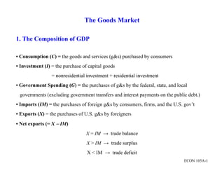
The Goods Market
1. The Composition of GDP
• Consumption (C) = the goods and services (g&s) purchased by consumers
• Investment (I) = the purchase of capital goods
= nonresidential investment + residential investment
• Government Spending (G) = the purchases of g&s by the federal, state, and local
governments (excluding government transfers and interest payments on the public debt.)
• Imports (IM) = the purchases of foreign g&s by consumers, firms, and the U.S. gov’t
• Exports (X) = the purchases of U.S. g&s by foreigners
• Net exports (= X IM)
X = IM → trade balance
X > IM → trade surplus
X < IM → trade deficit
3.
ECON 105A-3
2. The Demand for Goods
• The total demand (Z) for domestic goods
Z ≡ C + I + G + (X – IM)
• Let’s assume that:
i) There exist only one good;
ii) Firms are willing to supply any amount of the good at a given price P; and
iii) The economy is closed (X = IM = 0) so that Z ≡ C + I + G.
4.
ECON 105A-4
2.1 Consumption (C)
• Consumption depends on disposable income ( ).
• Notice that tax is lump-sum. Tax can take other forms too: e.g., tax as a function of income.
• In a functional form, and 0.
• One example of such a consumption function is
where is the marginal propensity to consume (MPC), 0 < < 1; and
is exogenous or independent consumption spending, 0 < .
6.
ECON 105A-6
2.2 Investment (I)
• For the time being, let’s assume investment is an exogenous variable: ̅
2.3 Government Spending (G)
• Government spending, G, together with taxes, T, describes fiscal policy.
• G and T are chosen by the government and so we also treat them as exogenous.
Note: I, G, and T are exogenous as they are assumed to be constant and do not vary in
response to a change in other variables in the model. C, on the other hand, is an endogenous
variable.
7.
ECON 105A-7
3. Equilibrium in the Goods Market
• Production (Y, which also measures income) is equal to the demand for goods (Z) in
equilibrium.
• The equilibrium condition: Y = Z
̅ ̅
⇒ 1 ̅
⇒
1
1
̅
i) The term ̅ is called autonomous spending.
ii) The term is called the multiplier. Why? Because of 0 1, 1.
8.
ECON 105A-8
• Understanding the Multiplier
Suppose 0.6 and increases by $1 billion. Then output increases by $2.5 billion.
The lesson we learn from here is that a change in autonomous spending will change output by
more than its direct effect on autonomous spending through the multiplier effect. Where does
the multiplier effect come from? Think about the following story. Suppose that someone
decides to spend $1 for the apple I have. At that moment, an increase in income is $1. But
that is not the end of the story. Having $1 as income now, I will spend of it, according to
my consumption function. The amount will go to whoever sells a product to me and that
person will spend . This process is likely to go on and on as there are a number of
sellers and buyers in the economy. So the total increase in income for the economy is:
1 ⋯
1
1
which is larger than the original $1 increase in income as long as 0 1. Hence the term
multiplier: the original $1 is ‘multiplied’ into a bigger amount $ .
11.
ECON 105A-11
• The process of equilibrium change above can be described as follows:
i) First of all, demand increases by $1 billion, shown by a shift from A to B.
ii) This first-round increase in demand leads to an equal increase in production, or $1
billion, also shown by the distance in AB.
iii) This first-round increase in production leads to an equal increase in income, shown by a
shift from B to C, where the distant BC also equals $1 billion.
iv) The second-round increase in demand, shown by the distance in CD, equals $1 billion
times the marginal propensity to consume ( ).
v) This second-round increase in demand leads to an equal increase in production, also
shown by the distance DC, and thus an equal increase in income, shown by the distance
DE.
vi) The third-round increase in demand equals $ 1 1 $ 1
2 billion.
vii) Following this logic, the total increase in production after, say, n + 1 rounds
1 ⋯ as → ∞
12.
ECON 105A-12
• In summary, an increase in demand leads to an increase in production and a corresponding
increase in income. The end result is an increase in output that is larger than the initial shift
in demand, by a factor equal to the multiplier.
4. An Alternative Way of expressing Goods-Market Equilibrium ( = )
• National Saving = Private Saving + Public Saving
i) Private Saving:
ii) Public Saving
When public saving > 0 , the government is running a budget surplus; and
when public saving < 0, the government is running a budget deficit.
iii) Go back to our equilibrium condition , which can be rewritten as
13.
ECON 105A-13
Using the definitions for private and public savings above, we have
(Private Saving + Public Saving = Investment)
• is called the IS relation. What firms want to invest must be equal to what
households and the government want to save.
14.
ECON 105A-14
• Consumption and saving decisions are the same:
1
where 1 is called the marginal propensity to save.
In equilibrium,
1
⇒ ̅ 1
⇒ ̅ 1
⇒
1
1
̅ G
15.
ECON 105A-15
• The Paradox of Saving
Suppose that, given disposable income , households decide to save more by lowering
Consumption (captured by ↓). Output ( ) would decline and private saving ( ) would be
unchanged in equilibrium. This paradoxical result is of much relevance in the short run.
16.
ECON 105A-16
Example 1: Goods market equilibrium output and saving
Z = C + I + G where C = 300 + 0.5YD, T = 400, I =200, G = 1000, YD = Y – T
a) Solve for equilibrium output (GDP). Compute total demand. Is it equal to production?
b) Write out the saving function for this economy. Then, calculate the level of private saving
that occurs at the equilibrium level of output.
c) Compute private plus public saving. Is the sum of private and public saving equal to
investment?
d) Suppose consumer confidence increases from 300 to 400. What is the change in output
level? What is the change in saving? Has this increased desire to consume had a positive
or negative effect on economic activity? How about on saving? Explain.