SlideShare a Scribd company logo
1 of 80
Download to read offline
11
VOLTAGE STABILITY
Mircea Eremia and Constantin Bulac
11.1 INTRODUCTION
Voltage stability is the power system ability to maintain the voltage level in acceptable
limits in all the buses, under normal operating conditions as well as after perturbations.
An electrical power system enters a voltage instability state when a disturbance-load
increase or change in the system topology-causes a progressive and uncontrollable
voltage level degradation in a node, in an area or in the whole system. In the first moments
the degradation process is slow, then it becomes more and more rapid, in general, if the
system operates near its transmission capacity. This limit is much lower in case of
unavailability of one generating unit or one component of the transmission network.
The main cause of the voltage instability phenomenon is the voltage drops due to
changes in the power flows through the inductive elements of the transmission network
following:
• load increase correlated with local or regional reactive power deficit;
• certain incidents that "weaken" either the local voltage control (tripping of some
generating units, exceeding some generators reactive power limits) or the transmis­
sion network (tripping of some transmission lines, transformers or autotransformers,
faults occurring on substations bus bars) orcause heavily loading ofthe transmission
network (separation of network), and so on;
• malfunction of on-load tap changing transformers.
Handbook ofElectrical Power System Dynamics: Modeling. Stability, and Control. Edited by Mircea Eremia and
Mohammad Shahidehpour.
© 2013 by The Institute of Electrical and Electronics Engineers, Inc. Published 2013 by John Wiley & Sons, Inc.
657
658 VOLTAGE STABILITY
Although, in essence, the voltage instability is a local phenomenon, its consequences
have a major impact on the system operation, sometimes initiating a voltage collapse
process.
The voltage "avalanche" or "collapse" phenomenon is characterized by a succession
of cascading events, associated with the instability phenomenon, that determine severe
reduction of the voltage level in an area or in the whole system and finally the loss of the
system angle stability.
Voltage collapse is typically associated with the reactive power demands of load not
being met because of limitations on the production and transmission of reactive power:
• limitations on the production of reactive power include generator and SVC reactive
power limits and the reduced reactive power produced by capacitors at low voltage;
• the primary limitations on the transmission ofpower are the high reactive power loss
on heavily loaded lines, as well as possible line outages that reduce transmission
capacity;
• reactive power demands of loads increase with load increases, motor stalling, or
changes in load composition such as an increased proportion of compressor load.
The voltage stability can be classified into:
• small-disturbance voltage stability;
• large-disturbance voltage stability.
11.2 SYSTEM CHARACTERISTICS AND LOAD MODELING
11.2.1 System Characteristics
Let us consider a simple radial network consisting of a source, a transmission line and a
load. Figure 7.1 shows the equivalent circuit and the phasor diagram. The characteristic ofa
system or transmission network "seen" from a load bus is the relationship between the
voltage at that bus and the delivered active and reactive powers, independent of the static
load characteristic.
Therelationship betweenthevoltages atboth ends ofthetransmission line, Y1 = VlID
and Y2 = V2ID, is obtained as follows:
V _
V
RP2 + XQ2 .XP2 - RQ2
-, - 2 +
V2
+}
V2
(1 Ll)
where R = Z cos f3 and X = Z sin f3 are the resistance and reactance, respectively, corre­
sponding to the equivalent impedance � of the transmission line.'
-22 = P2 +jQ2 = S2(COSq! +j sinq!) = V2 [
*
L The European standards use letter "u' to denote the phase-to-phase voltage (called also line-to-line voltage); for
compatibility with the North American standards, in this chapter we will use letter " V", and the expression
§. = P +jQ = .Y!..* stands for the three-phase complex power.
SYSTEM CHARACTERISTICS AND LOAD MODELING
Taking into consideration the phasor diagram from Figure 7.1, by separation ofthe real
and imaginary parts of (1 Ll) yields:
V1V2COS e = V�+ RP2 + XQ2 (l 1.2a)
VIV2sin e = XP2 - RQ2 (11.2b)
To eliminate e, the sum of squares of equations (l1.2a) and (1 1.2b) is computed,
resulting:
or
where
( )2 ( )2 2 (2 2) 2 2
RP2 + XQ2 + XP2 - RQ2 = Z P2 + Q2 = Z S2
Equation (11.3) can be written as:
f(V2, P2, cP) = vi + [2S2(R cos cp + X sin cp) - VTlV�+ Z2S� = 0
(11.3)
(11.4)
which defines the implicit relationship betweenthe receiving-end voltage ofthe transmis­
sion line V2 and the transmitted powers P2 and Q2. Starting from this equation, the voltage
V2 can be expressed as an explicit function:
V2 = g(P2, Q2) = g(S2, cp) (11.5)
that defines the system or transmission network characteristics represented by the surface
from Figure 11.1.
The explicit function defined by expression (1 1.5) may exist only if the biquadratic
equation (11.4) obeys the implicit functions theorem conditions, that is, to have real roots.
This condition is fulfilled if the discriminant Ll is positive:
(11.6)
At the limit, when the discriminant Ll is equal to zero, gives
2S2(R cos cp + X sin cp) - VT = ±2ZS2
or
2S2(R cos cp + X sin cp ± Z) = VT
659
660
thus:
V2
S2 = 1
2(R cos cp + X sin cp ± Z)
VOLTAGE STABILITY
2Z[cos(,B - cp)± 1]
(11.7)
Because S2 > 0, the positive sign "+" at the nominator of equation (1 1.7) holds,
therefore, the maximum loadability of the line:
V2
S2max = 1
2Z[cos(,B - cp)+ 1] 4Z cos2[(,B - cp)j2]
(11.7')
thus resulting the same expression (8.6), previously computed following a different path
(see Section 8.2.2), respectively:
VI cos cp
P2max = -:-
4Z
=--
CO-S """
2[
'-;- (,B
-::---'
_
'-
cp
""7
)
""7C
j2
'"'"
]
(11.8)
11.2.2 Load Modeling
11.2.2.1 Load Characteristics. Voltage stability, also known as "load stability," is
strongly influenced by the static characteristics and the dynamic response of the load [1].
as:
In the power systems terminology, the term "load" can have different meanings, such
(i) a device connected to the power system that consumes active and/or reactive
power;
(ii) the total active and/or reactive power consumed by all devices connected to the
power system;
Asynchronous
motors
("'T;����;�;i'��'�'����;k""'!
! (llOkV) I
" ....____ ____•••__....__________ ---_____,1
f1Capacitor banks
t--
.... Lighting
Resistive
loads
Figure 1 1 . 1 . The load structure of a transm ission network bus.
SYSTEM CHARACTERISTICS AND LOAD MODELING
(iii) a part ofthe power system, which is not explicitly defined, but it is assigned as a
device connected to the power system.
The driving force for voltage instability is usually the loads. After a disturbance, load
power restoration is attempted by motor slip adjustment, tap changing, and thermostats.
Generally, the load modeling is an important issue, since in a power system the loads
are aggregated, that is, they consist of different receivers. The main problem is the
identification of the load components at a given instant and their mathematical represen­
tation. To understand the nature of the dependence between voltage stability and load
dynamics, it is necessary to analyze the load in an individualistic approach. For this
purpose, this section focuses on the dependence between voltage and load, especially on
the properties of the exponential and polynomial load models.
In power system stability studies, in general, and in voltage stability, in particular, the
meaning of load is taken as the definition (iii), representing a distribution network that
receives power from the transmission network through a substation. Therefore, the load
connected to a bus, also known as complex load, includes, besides individual consumers
(synchronous and asynchronous motors, resistive loads, etc.), the feeders, distributors,
transformers, and so on (Figure 11.1).
The load characteristics are a set ofparameters, such as the power factor or variation
of active and reactive powers with voltage and frequency, that characterize the specific
behavior of the load in static or dynamic states. The load mathematical model can be
formulated in the general form as Ref. [3,51,52]:
P = Kp . Po ·
fp(V,j)
Q = KQ . Qo ·
fQ(V,j)
(11.9)
where Po, Qo are the active and reactive load powers, for values of voltage and frequency
corresponding to the normal operating state (Vo,fo); Kp, KQ are the independent quantities,
known as load demand coefficients; andfp,fQ are the functions expressing the dependency
of the active and reactive load powers on the voltage and frequency at a given time.
In steady state, the load characteristics, called static load characteristics, representthe
dependency at a given time ofthe active andreactivepowers on the connection bus voltage
and the system frequency in quasi-static state. This state is characterized by very slow
modifications of the operating conditions, and the transition from one state to another can
be considered a series of steady states (a series of equilibrium points). The modeling of
these characteristics involves only algebraic equations.
In dynamic state, the load characteristics, called dynamic load characteristics, also
represent the dependency of the active and reactive powers on the connection bus voltage
and the system frequency, but in transient state, when the operating conditions substantially
changes from one instant of time to another.
As general simplification, for voltage stability studies, the frequency dependency of
the active and reactive powers is neglected, and therefore the general load mathematical
model can be written as:
P = Kp . Po ·fp(V)
Q = KQ . Po ·fQ(V)
(11.10)
Unlike the system characteristics, where the amounts ofthe active and reactive powers
that can be delivered to the load zone, the load characteristics define the variation of the
661
662 VOLTAGE STABILITY
active and reactive powers in terms of the receiving-end voltage of the transmission line.
For the considered configuration, this dependence can be written as:
P2 = fp(V2, Po,2)
Q2 = fQ(V2, Qo,2)
(1 1.11)
where P2 and Q2 represent the demanded powers under certain operating conditions.
The last expressions define, in the (Vz, P2, Q2) space, a curve that, for a specific
power demand, which does not exceed "the capability of the transmission network,"
intersects the surface defined by equation (11.5) in one or more points representing
possible operating points. When the demand changes, these points move on the surface
and their projection in the (V2, P2) plane represents the V2-P2 characteristic of the
system (transmission network). Note that the system characteristic cannot be defined
without specifying how the power delivered to the load varies. Therefore, the Vz-P2
characteristic corresponding to a constant power factor represents a particular case of
system characteristic.
11.2.2.2 Static Models. EXPONENTIAL MODEL. This is one of the most used models,
having the general form:
(v)ap
P = Kp' Po' Vo
(l1.12a)
(l1.12b)
whereKp andKQare dimensionless load coefficients, being equal to 1 forthe base case; Vo
is the reference voltage; and C¥p, c¥Q are the coefficients depending on the load type.
The terms Kp. Po and KQ . Qo represent the absorbed active and reactive powers,
respectively, at avoltageVequal tothereference voltageVo, andcorrespond tothenominal
load powers.
It is necessary to make distinction between the actually consumed power andthe load
demand. This distinction is important for understanding the basic instability mechanism,
since as the load demand increases theconsumedpowermay decrease, as a consequence of
the voltage decrease.
Three particular cases for C¥p and c¥Q are usually considered as follows:
• constant impedance load: C¥p = c¥Q = 2
• constant current load: C¥p = c¥Q = 1
• constant power load: C¥p = c¥Q = 0
For lower voltage values the exponential model is not sufficiently precise, because,
when the voltage drops below a certain value (e.g., V :s; O.6p.u.), many consumers are
disconnected or their characteristics are completely altered.
Two of the most important properties of the exponential model are presented.
(i) Toinitialize theexponentialmodel, any voltage level can be used as reference. To
demonstrate this property Kp = 1 is considered, while the reference voltage Vo
SYSTEM CHARACTERISTICS AND LOAD MODELING
and the powers Po and Qo can be arbitrarily specified without changing the
characteristic. Thus, for a voltage level VI, we have
If Po is expressed from the last equation then replaced in (l 1.12a) results:
(V)<XP
P = P1• �
Thus, Vowas replaced with VI and Powith P], and the new reference voltage
becomes VI'
(ii) The exponents ap and aQ used in the load exponential model determine the
powers sensitivity to voltage change. ConsideringVo as reference voltage and Po
the active power load corresponding to this voltage value, the power sensitivity to
voltage change can be calculated as:
dP (V)<XP-l
dV = ap' Po' Vo Vo
Evaluating the sensitivity for V = Vo obtain as follows:
respectively
dP/Po
---
-a
dV/Vo- p
dQ/Qo
----a
dV/Vo- Q
(l1.13a)
(11.13b)
Therefore, the sensitivities have the same values irrespective of the voltage
reference value. The expressions (equation l 1.13a,b) can be written as:
IlV
IlP = ap-Po
Vo
IlV
IlQ = aQ-Qo
Vo
If the pervious equations are divided member by member, gives:
IlP ap Po
IlQ aQ Qo
Giventhe relationship Q = p. tanrpiftanrp = tanrpo = ct.(tanrpo = (Qo/Po))
obtain as follows:
meaning that for constant power factor, ap=aQ.
POLYNOMIAL MODEL. Since different components of a complex load present different
voltage characteristics, an alternative load model obtained by summing up the load
663
664
TAB L E 1 1 .1 . Polynomial Load Models (3)
Load Type
Air conditioner
Asynchronous motors
Complex load 0.83 - 0.3 (fo)+ 0.74 (fo)2
VOLTAGE STABILITY
2.08+ 1.63 fo - 7.6 (fo)2
+ 4.89 (for
6.7 - 15.3 (fo)+ 9.6 (for
components, which presents the same (or almost the same) exponent, should be considered.
When all exponents are integers, the load characteristic becomes a polynomial function
of V.
A special case is the load model consisting ofthree components: constant impedance,
constant current, and constant power. In this case, the characteristics of the active and
reactive power, respectively, of the load model are given by the expression [2]:
P = Kp. po· [ap. (:J2 + bp .:0+ cp]
Q = KQ. Qo· [aQ . (:J2 + bQ .:0+ CQ]
(1 1.14)
where ap, bp, Cp, aQ , bQ, cQ represent the weights of each component and satisfy the
relationships ap + bp + Cp = 1 and aQ + bQ + cQ = 1; and Kp. Po, KQ. Qo are active and
reactive consumed powers, corresponding to the reference voltage Vo.
Similar to the exponential model, for reduced voltage values, the polynomial model
cannot be used to appropriately model the loads.
Table 1 1.1 shows some polynomial models [3].
11.2.2.3 Dynamic Models. These models describe, through algebraic-differential
equations, the dynamic behavior of the load given either by the intrinsic load character­
istics orby the actions ofsome control devices such as the automatic on-load tap changer or
the thermostat load control systems.
Because the use of physical dynamic models specific to some loads, such as large
synchronous and asynchronous motors individually represented, is inadequate forcomplex
load modeling, the so-called generic dynamic models have been developed. They describe
the specific behavior of the complex load when subjected to sudden voltage variations in
the connecting node, due to various disturbances occurring in the transmission network.
The measurements at the HV bus bars of some substations supplying the distribution
network showed that the response of the complex load to sudden voltage variations is as
illustrated inFigure 11.2 fora real power P [4]. This response reflects the collective effects
of all the complex load components, from the on-load tap changer to the individual
household loads (Figure 1 1.1). The time span for a load to recover to steady state is
SYSTEM CHARACTERISTICS AND LOAD MODELING
(a) V (b)
P
Po
P, - - - - - - t-------;-:--::��
-- '
P.,o
Figure 1 1 ,2, The dynamic active power response of a complex load (b) at sudden voltage
variation in the connection node (a) [4],
normally in the range of several seconds to minutes, depending on the load composition,
Responses for real and reactive power are qualitatively similar.
It is obvious that a sudden voltage variation determines an instantaneous change in the
consumed power. This variation defines the transient characteristic o/the load and can be
modeled as constant impedance �n as used in the transient stability analysis tools, or,
more general, as an exponential characteristic. A dynamic load restoration process follows
characterized by an increase in the power demand up to a new voltagevalue on the steady­
state characteristic.
On a longer timescale, the lower voltage tap changers and other control devices act to
restore voltages and so the load. In fact, the aggregate effect ofdistribution-Ievel restoration
can be to cause load overshoot. With recovery time (Tp) on a timescale of a few seconds,
this behavior captures the behavior of induction machines. On a timescale of minutes, the
role oftap changes and other control devices is included. Over hours, the load recovery and
possible overshoot may emanate from heating load [4].
The dynamic restoration process can be asymptotic or even oscillatory (Figure 1 1.2b)
and can be modeled through a set of differential equations [2]:
(11.15)
where Po, Qo are the active and reactive consumed powers in normal operating state
characterized by the voltageVo; Ps, Pt are the steady-state and transient load characteristics
of the active power; Qs, Qt are the steady-state and transient load characteristics of
the reactive power; Xp, XQ are the generic dimensionless state variables associated
with the load restoration dynamic process; and Tp, TQ are the load restoration dynamic
process.
The generic models are usually associated with the exponential load models. Hence,
the steady-state characteristic is given by expressions (1 1.12) where Kp = KQ = 1:
(V )ap
Ps = Po' Vo ; (1 1.12')
Depending on the way in which the generic variables Xp and XQ intervene in the
expressions of the transient load characteristics, there are two types of generic dynamic
665
666 VOLTAGE STABILITY
models: the additive model where the generic state variables are appended to the transient
characteristic and the multiplicative model where the generic state variables multiply the
transient characteristics.
(i) The additive generic model
The transient load characteristic is given by [2]:
(1 1.16)
where Q'P,I and Q'Q,I are exponents of the transient load characteristics.
Hence, the differential system of equations (11.15) describing the load
restoration dynamic process becomes:
dXp 1 (V)<XP (V)<XP"
Tp-=-(Ps -PI) = - - - -Xp
dt Po Vo Vo
dXQ 1 (V)<XQ (V)<XQ,'
TQ-=-(Qs -QI) = - - - -XQ
dt Qo Vo Vo
(ii) The multiplicative generic model
The transient load characteristic is given by:
PI =Xp .Po' (V/Vo)"P"
(1 1.17)
(1 1.16')
and the differential system of equations (11.15) describing the load restoration
dynamic process becomes:
Tp
dXp
=�(Ps -PI) =(V/Vo)"P -Xp .(V/Vo)"""
dt Po
TQ
dXQ
=�(Qs -Qt) = (V/Vo)"Q -XQ . (V/Vo)"Q,'
dt Qo
(1 1.17')
The following remarks are made regarding the two generic dynamic models [2]:
(i) the exponents Q'P,t and Q'Q,t have usually large values and thus the dependence on
voltage of the load powers is greater in transient state than in steady state;
(ii) the generic state variablesXpandXQ must range within acceptable limits, that is:
Xwin :s Xp :s XWax
XQin :S XQ :S XQax
(1 1.18)
(iii) the constant power type component introduced in the additive models may cause
nonphysical singularities to the transient characteristic, which is not the case for
the multiplicative model;
STATIC ASPECTS OF VOLTAGE STABILITY
(iv) the simple model given in(I1.12') can be obtained ifwe take Xp = XQ = O in the
additive model, and Xp = XQ = 1 in the multiplicative model, respectively;
(v) the exponents Q'p and Q'Q and the time constants Tp and TQ can be determined
using measurements of powers supplied to the distribution network either
considering disconnection of a transformer or on-load tap changing in the
HVIMV distribution substation leading to gradual modification of the voltage
level Ref. [2].
11.3 STATIC ASPECTS OF VOLTAGE STABILITY
11.3.1 Existence of Steady-State Solutions
The projection of the points corresponding to the maximum transmissible power S2max
in the (P2, Q2) plan determines a curve that separates the plan into two zones (see
Figure 1 l .3) [5]:
The hatched zone represents the domain of existence of solutions and corresponds to
the possible operating points (A and B in Figure 11.4), for which the biquadratic equation
(11.3) has two distinct real positive solutions.
Using the notations:
y = V� Q' = vf - 2(RP2 + XQ2)
Ii = [2(RP2 + XQ2) - Vf]
2
- 4Z2(p� + QD
from (1 1.3) a quadratic equation in y is obtained as follows:
v,
0,
Geometrical locus
of the critical points
of the solutions
(1l.3)
(1l.l9)
Figure 1 1 .3 . The dependence between the voltage V2 and the powers P2 and Q2< for a simple
generator-li ne-load config u ration.
667
668
v,
�
Controllable zone
VOLTAGE STABILITY
�,max 1-----.:;:",.___ : A
Security zone Critical
�,m
in I----------!---..::......
/ point
Critical zone
v"cc '-----------!------.
, I.C
;;;
I'
I •
I •
" .
" .
.�......... �
;; : B :
;;;
�
�---T------�--�
Uncontrollable zone P, P2mo>
Figure 1 1 .4. The VrP2 system characteristic:
operating poi nts,
with the solutions Yl,2' which give the voltages corresponding to the two possible operating
points A and B:
v -
Ja+ JI5.,
2A -
2 '
V2B =
Ja-
JI5.
2
(11.20a,b)
• The external zone represents the domain of inexistence of solutions, thus no
operating points are found in this area.
• The critical points situated on thefrontier represent static bifurcation points for the
system evolution as they are characterized by zero value of the discriminant from
equation (11.19), Ll = 0, of the biquadratic equation (11.3), resulting:
If Ll = 0 is considered in the expressions (11.20a and b), identical solutions V2A and
V2B are obtained in the critical points, corresponding to the possible operating points:
VI - 2(RP2max +XQ2max)
2
(1 1.21)
Note that in the critical points situated on the separation frontier of the domain of
existence of solutions in the P2-Q2 plan, the Jacobian matrix of the Newton-Rhapson
method-based loadflow mathematical model become singular.
We know that:
11
Pi = GuV7 + LViVkGGik
k=l
keFi
OPi 2 � 2 2 � 2
oVi
Vi = 2GUVi + � VYkGGik = GUVi + GUVi + � ViVkGGik = GUVi +Pi
k=l k=l
STATIC ASPECTS OF VOLTAGE STABILITY 669
where
OPi Pi + GiiV?
oVi Vi
n
Qi = -BuV? - LVYkBBik
k=1
k#i
OQi 2 ...f- 2
oVi
Vi = -2BuVi - � VYkBBik = -BUVi +Qi
k=1
k#i
OQi Qi - BiiVf
oVi Vi
The Jacobian matrix of the power system from Figure 7.1, considering that the bus 1
(the slack bus) voltage is taken as phase reference with Y1 = VI lei = 0 , and the bus 2
voltage is Y2 = V2 lti2 ' has the following form:
where
OP2 _
P2 + G22V�.
oV2 V2 '
Thus, the determinant of the Jacobian matrix is
670
Because in the critical point vi = vier = Z2 .S�, it results:
det[i] = 0
VOLTAGE STABILITY
This property, valid for a simple generator-line-load configuration as well as for any
complex network, is the core of voltage instability and collapse risk assessment, due to the
inexistence of the equilibrium points (steady-state solutions) caused by load increase
and/or due to the contraction of the domain of existence of the solutions after a
contingency.
11.3.2 Operating Points and Zones
For analysis ofthe points inside the hatched zone (Figure 1 1.3), the dependence between P2
and Q2 through the power factor cosrpis considered. Thus, equation (11.4) can be written
as:
vi + [2P2(R + Xtanrp) -vf] V� + Z2 (�)
2
= 0
cosrp
(1 1.22)
If VI and cosrp are considered constant, then for values of the active power
P2 E [0, P2max], an expression ofthe form V2 = f(P2), called the V2-P2 "system character­
istic," can be obtained (see Figure 11.4) [5].
Figure 11.4 shows that for a transmitted power P2 ::; P2max, two possible operating
points are found as: point A, characterized by a high-voltage value, corresponds to the
normal operating conditions being a stable operating point, whereas point B, characterized
by a low-voltage value, corresponds to abnormal operating conditions.
To demonstrate why A is stable and B is unstable, the effects of voltage regulation by
the control ofthe power factor at the transmission line receiving end and voltage variation
at the transmission line sending-end will be analyzed.
v,
(i) The effect of compensating the transmitted reactive power
Considering different values for cosrp and keeping constant the sending-end
voltage of the transmission line (VI = ct.), the family of V2-P2 characteristics
from Figure 11.5 is obtained.
For a given value P2 < P2max, the V2A voltage corresponding to the operating
point A increases as the power factorchanges from inductive to capacitive values.
Atthe same time, inthe point B, compensation ofthe reactive power has opposite
cos cp = 0.95 lag
cos cp = 1.0
� r-o:::::::::I=:::t:::-f-- cos cp = 0.95 lead
power factor
v cap
2,cr
V
ind
2,cr
P,
Locus of
critical points
P,
Figure 1 1 . 5. Effect of reactive power com­
pensation on the VrP2 characteristic.
STATIC ASPECTS OF VOLTAGE STABILITY
q,
1 0.75
T 0.50
0.25
effects since the voltage decreases as cos cp changes from inductive to capacitive
values. Therefore, point A is a controllable operating point and thus stable;
whereas point B is uncontrollable and thus unstable.
The locus of critical operating points is shown by dotted line in Figure 11.5.
Normally, only the operating points above the critical points represent satisfac­
tory operating conditions. Thus, a sudden reduction in the power factor (increase
in Q2) can cause the system to change from stable operating conditions to
unsatisfactory, and possibly unstable, operating conditions represented by the
lower part of a V2-P2 curve.
The influence of the reactive power characteristics of the equipments at the
receiving end (loads and compensating devices) is more obvious in Figure 11.6
[6], which shows a family of curves applicable to the power system from
Figure 1 1 .4, each of which representing the relationship between V2 and Q2 for
a fixed value of P2.
For a complex system, these curves can be obtained for a load bus through
repeated load flow calculations. In this regard, consider that a virtual reactive
power source (without power limits) is connected to the bus. As a consequence,
thisbusbecomes aPVbus where the voltage is imposed and the reactive power is
calculated.
An example of this type of characteristics, in p.u., q = QX/V�, is given in
Figure 11.6 for a transmission line (X » R) having an active source as parameter
(p = PX/VT) and a switched capacitor bank.
The system is stable in the region where the derivative dQ2/dV2 is positive.
The voltage stability limit (critical operating point) is reached when the deriva­
tive is zero. Thus, the zones on the Q2-U2 curves to the right of the minima
represent stable operation, and the zones to the left represent unstable operation.
Stable operation in the region where dQ2/dV2 is negative can be achieved only
with a continuously regulated reactive power equipment that has sufficient
control range and high QIV gain with polarity opposite to that of the normal.
If no capacitor bank is connected, the operating point is at the intersection of
the V-Q characteristic with the horizontal axis (Figure 11.6, the a curve). If
reactive power compensation is provided, a new operating point can be found at
the intersection between the bus characteristic and the capacitor bank character­
istic (Figure 11.6, curves b and d). Notice that for large values of the transferred
active powers, if there is insufficient compensation, no operation point can be
defined.
Operating point
Operating point
O�������-.--+�
' Reserve in MVAr
without capacitor (case )
-0.25 --"":------'---
Figure 1 1 .6. The Qru2 cu rves for vari­
ous real-power load [6, 51).
671
672 VOLTAGE STABILITY
V,
The reactive power reserve to maintain normal operation is the distance, in
MVAr, from the operating point to the minimum ofthe bus characteristic (Figure
11.6, case 1), without capacitor, or to a point where the capacitor bank
characteristic on the lowest step is tangent to the bus characteristic (Figure
11.6, case 2).
The slope ofthe characteristic in the operating point is the aQ/aV sensitivity
that shows the robustness or weakness of the analyzed bus as well as the
effectiveness of reactive power compensation.
(ii) The effect of controlling the transmission line sending-end voltage
Considering different values for the transmission line sending-end voltage,
Vii) and V(2), obtained by modifying the generator's field current, and constant
powerfactor (cos c:p = ct.), thefamilyof V2-P2 characteristics from Figure 11.7 is
obtained.
In this case, for a constant value P2 < P2max of the transmitted active power,
the point A is a normal operating point because the corresponding voltage (VA)
increases as the transmission line sending-end voltage increases. In exchange, the
point B is an abnormal operating pointbecause the sending-end voltage increases
as the voltage corresponding to this point decreases.
Therefore, the control of VI voltage at the transmission line sending­
end through change of the generator's field excitation current has the desired
effect on the operating point A, while for the operating point B the effect is
opposite.
Moreover, analyzing the characteristics from Figures 1 1.5 and 11.7, we can
see that the critical voltage and the maximum transmissible power increase as the
reactive power is compensated with the help ofreactive power devices, or as the
transmission line sending-end voltage increases. When operating near the limit,
the two voltages corresponding to the possible operating points will have high
and closed values. Therefore, the voltage attached to one operating point only is
not an indicator of voltage instability proximity. Additional information such as
voltage sensitivities to active and reactive powers variation is thus necessary.
(iii) Voltage sensitivities to active and reactive powers variation
The voltage sensitivities can be obtained by differentiating equations (11.4).
To simplify the calculus, a small phase difference between the voltage phasors at
the transmission line ends is assumed, that is, 8 = (81 - 82) � O. Therefore,
using equations (1 1.2a) and (11.2b), since cos 8 � 1 and sin8 � 0, equation
(1 1.3) becomes:
11,')
r----l-<'----
0')
1
11,(1) r-_-'-
""""__--'-___'cc-_--,'::-+ P, Figure 1 1 .7 . The effect of controlling the voltage V,
P, on the VrP2 characteristic.
STATIC ASPECTS OF VOLTAGE STABILITY
The voltages corresponding to the possible operating points A and B are
as follows:
VI + VVI -4(RP2 +XQ2)
V2A � --
--'-----
----:,--------
2
(l1.23a)
VI - VVI -4(RP2 +XQ2)
V2B � ----'------:,--------
2
(1 1.23b)
A power system, seen from a bus i, is stable from the viewpoint of the
bus voltage, if the addition of a conductance aGi or a susceptance aBi,
respectively, eventually infinitesimal, determines the increase in the consumed
active and reactive powers, and a simultaneous decrease in the voltage of the
considered bus. Therefore, the necessary and sufficient condition for the power
system to be controllable is [7]
-
<0'
dVi
I
dGi Bi=ct
'
dVi
I 0
- < .
dBi Gi=ct
'
-
>
dPi
I 0
dGi Bi=ct
- >
dQi
I 0
dBi Gi=ct
(11.24)
The sensitivities 2 ofvoltage tothe activeandreactive powers intheA and
B points can be calculated starting from the expressions (11.23a,b):
-4R -R
2 · 2VVT -4(RP2 +XQ2)
-----r====== <0
VVT -4(RP2 +XQ2)
8V2A
I
-x
8Q2 PFct
=
VVT _ 4(RP2 +XQ2)
<0
R
-----,=-====== > 0
VVT -4(RP2 +XQ2)
2 If y = VuW then y
' =
� or <!l =
�
2�'
du 2�
(l1.2Sa)
(1 1.2Sb)
(l1.2Sc)
(l 1.2Sd)
673
674 VOLTAGE STABILITY
According to the definitions from (1 1.24) and (1 1.25), point A is a controlla­
ble operating point, thus stable, and point B is an uncontrollable operating point,
thus unstable.
Considering these aspects, the following operating zones can be defined on the V2-P2
characteristic (Figure 11.4):
• The Controllable Zone. Corresponds to the upper side of the characteristic and
comprises the operating points forwhich Zc > Zand sensitivities are negative. In the
technical literature, this zone is known as the stable operating zone. If the critical
voltage is lower than the minimum admissible operating voltage (Vmin), this zone can
be divided into two subzones:
- The Security Zone. Defined between the maximum and the minimum admissible
voltages (Vmin and Vmax), characterized by negative and close to zero
sensitivities;
- The Critical Zone. Defined between Vmin and Vcr voltages, characterized also by
negative sensitivities but high in magnitude. Depending on the load characteristic,
operation in this zone can trigger voltage instability phenomenon or voltage
avalanche, phenomenon characterized by a voltage decrease towardVcr. either due
to an increase in the power demand or due to the on-load tap changing transform­
ers action.
• The Uncontrollable Zone. Corresponds to the lower side of the characteristic and
comprises the operating points characterized by Zc < Z and positive sensitivities.
This zone is known in the technical literature as the unstable operating zone.
Note that the assumption of a small phase difference (e small) is no longer possible to
determine the critical voltage because, if in equations (1 1.23a,b) the zero condition of the
discriminant would be imposed, the critical voltage is obtained Veri! = VJ/2, value that
depends on the sending-end voltage but is independent of the power factor, which is in
contradiction with the remark previously made.
11.4 VOLTAGE INSTABILITY MECHANISMS: INTERACTION BETWEEN
ELECTRICAL NETWORK, LOADS, AND CONTROL DEVICES
In power systems operation, the maximum transmissible power and the critical voltage
are only for theoretical importance since they cannot be precisely determined due to the
phenomenon complexity, depending on a series of factors influencing each other (load
behavior, keeping the voltage to the reference value in the generator nodes, the reactive
power compensation devices action, etc.).
11.4.1 Interaction between Electrical Network and Load
There are two basic mechanisms that can lead to voltage instability and collapse
phenomena in power systems. One of these mechanisms is the slow increase in the
load demand, and the other one resides in the disturbance occurrence in the transmission
network (disconnection of electrical lines, transformers, generators, etc.) that lead to the
modification of the V2-P2 characteristic.
VOLTAGE INSTABILITY MECHANISMS: INTERACTION BETWEEN ELECTRICAL NETWORK
(a) V, Load increase
V,r-_-J
B
(b) V,
Load increase
� r--_�
.
P,
P2,m
ax -
Figure 1 1 .8. Voltage instabil ity mechan ism i n terms of load demand i ncrease: (a) P= ct;
(b) voltage-dependent load.
(i) The voltage instability phenomenon mechanism, caused by the load increase,
considering different static load characteristics, is illustrated in Figure 1 1.8.
• Thus, for a P= ct. load characteristic, as the demand power increases, due to the
load characteristic shifting, the two equilibrium points approach each other,
overlap in the critical point C (which represents a singular point coinciding, in this
case, with the maximum transmissible power) and then disappear (Figure 11.8a);
• Ifthe load is representedby exponential model, and the operating point is situated
on the upper side, as the load demand increases, this point moves from AI to A2
(Figure 1 1.8b) leading to voltage decrease simultaneously with increase in the
transmitted power, which corresponds to a normal operation ofthe "transmission
network-load" configuration. Instead, if the operating point is situated on the
lower side, as load demand increases, the point moves from B1 to B2 causing a
decrease both in the voltage level and in the transmitted power, which corresponds
to an abnormal operation of the transmission network-load configuration.
(ii) The voltage instability mechanism to a major disturbance, caused by dis­
connection of one circuit of the transmission line, is shown in Figure 11.9.
The disturbance occurrence causes inthe first moments a decrease involtage and
therefore sudden decrease in the load demand, in accordance with the transient
load characteristic, and the operating point moves from Al, situated on the
normal operation characteristic, to A2, situated on the postdisturbance charac­
teristic. As the transient process evolves, the point A2 moves toward a new
equilibrium point, given by the intersection between the static load characteristic
and the postdisturbance characteristic ofthe transmission network. We see that, if
the load is of P= ct. type there is no intersection point between the two
characteristics, which determines the voltage to collapse at the load terminals
(Figure 1 1.9a).
Instead, if the load is represented by exponential model, the two characteristics
intersect in point A', which is the new operating point characterized by a reduced
voltage level (Figure 1 1 .9b-curve a) (see also Section 8.2.2). However, in this case, the
voltage collapse can be triggered by the on-load tap changer actions, trying to restore
the voltage to the reference value. The consequences of this action are the change of
the load characteristic seen from the transformer primary and the increase in the
consumed power from the system, which increase the risk for voltage instability and
voltage collapse (Figure 1 1 .9b-curve b).
675
676
(a)
V,
Postdisturbance Predisturbance
characteristic characteristic
�=-------�---.�
(c)
0.0
(b)
B
Po
VOLTAGE STABILITY
Postdisturbance
v, characteristic Predisturbance
""""=-------�---. P,
Postdisturbance
system curve
C
1.0
P
Figure 1 1 .9. The voltage instabil ity mechan ism to major d istu rbances (a and b) and the reg ion of
attraction (c).
These mechanisms caused by the load behavior are strongly influenced by the on-load
tap changer action, a reactive power deficit due to limitations in the generator's field and
armature currents, as well as following the secondary voltage control system actions.
The portion of the V-P characteristic that allows restoring the system operation to a
stable equilibrium point is called region of attraction (Figure Il.9c). Consider the
simplified radial power system with constant sending-end bus voltage and unity power
factor load. As shown before, there are two possible equilibrium points corresponding to
Po = ct: point A situated on the upper section of the V-P curve, which is a stable
equilibriumpoint, and point B situated on the lower section ofthe V-P curve, which is an
unstable equilibrium point (Figure Il.9c).1t can be shown that, after a disturbance, ifthe
power system reaches an operating point situated anywhere on the DACB section of
the V-P characteristic, appropriate measure can help increasing the voltage and thus
moving the system operation in a stable equilibrium point corresponding to the
demanded power. [8,9].
11.4.2 Influence of the On-Load Tap Changer
In some power system operating conditions, the on-load tap changer actions performed
under an automatic voltage regulator (AVR) may enhance the risk for or even trigger the
voltage instability process [10]. To analyze this phenomenon, let us consider the one-line
diagram fromFigureII.lOa ofa system supplying through a shortelectrical line and an on­
load tap changing (OLTC) transformer equipped with AVR.
11.4.2.1 Modeling the On-Load Tap Changing Dynamics. Neglecting the
transformer no-load losses, including its series impedance in the equivalent impedance �
and modeling the load by the impedance �c, the equivalent circuit from Figure Il.lOb is
obtained.
VOLTAGE INSTABILITY MECHANISMS: INTERACTION BETWEEN ELECTRICAL NETWORK
(a)
P,+jQ,
Figure 1 1 . 1 0. One-l ine d iagram (a) and equ iva lent circu it (b) for the analysis of the on-load tap
chang ing influence.
The turns ratio N is a real number given by:
(11.26)
where Vnp is theprimary winding nominal voltage (the nominal voltage ofthehigh-voltage
winding, equipped with tap changer); Vns is the secondary winding nominal voltage; np is
the actual tap position (actual operating tap); and LlVp is the percentage ofvoltage variation
per tap (expressed in percents).
The turns ratio N varies within the admissible interval [Nlo, Nup] given by the
transformer's control capability (number of taps).
The role of AVR is to change on-load the ratio N so that the load side voltage V2 is
kept inside the interval [V2,sch - 8, V2,sch + 8], called the insensitivity domain of the
regulator, around the reference voltage V2,sch, determined under stable-operating
conditions. Therefore, if the load side voltage is lower than V2,sch - 8 then, after a
period called delay period, according to expression (11.26), written as V2 = V2'/N, the
regulator will command the tap change with one position in the sense of turns ratio
decrease, resulting the increase of V2. Reverse, if V2 > V2,sch + 8 the regulator will
command the tap movement with one position in the sense of turns ratio increase,
resulting the decrease of V2, The process will continue until either the voltage is brought
back within the admissible interval or one of the limits, Nlo or Nup, is reached (the tap
changer reaches one of its extreme positions).
The dynamic behavior ofan on-load tap changing transformer equipped with AVR can
be described using either a discreet model or a continuous model.
• The discrete model assumes that the regulator, activated whenever the load side
voltage does not fulfill the condition IV2 - V2,sch I :::; 8, will command the tap change
at discrete time intervals tko k = 0, 1, . . . , n, which satisfies the recursive formula:
tHI = tk + LlTk and to = O. In this expression, LlTk denotes the time delay and
depends on the regulator characteristics and the voltage error, Generally, LlTk is not
necessarily constant and may be determined using the expression [2]:
8
LlTk = Td
I I
+ Tf + Tm
V2 - V2,sch
(11.27)
where Td is the maximum time delay of the inverse time characteristic; Tf is a fixed
value ofthe time delay; T.n is the mechanical time necessary to perform the tap change;
and E is half of the OLTC deadband,
677
678 VOLTAGE STABILITY
The tap changing logic, called direct or normal logic, can be defined as:
V2 < V2sch - 8 and Nk > Nlo
IV2 - V2schI :s; 8
V2 > V2sch + 8 and Nk < Nup
(1 1.28)
where � is the size of tap step and Nup, N,o are the upper and lower tap limits.
• The continuous model assumes a continuous variation of the turns ratio N(t) within
the interval [N,o, Nup] and ignores the insensitivity domain of the regulator.
Therefore, the tap changer dynamics can be modeled through the following
differential equation:
dN 1
- = --(V2 - V2sch)
dt TAVR
where TAVR is the time constant of the regulator.
(1 1.29)
Although the continuous model is less accurate than the discrete model, it is more
frequently used in the technical literature because it allows the analytical investigation of
the tap changing behavior and highlights the influence on the voltage stability [2].
11.4.2.2 The Effect ofAutomatic Tap Changing on the Possible Operating
Points. It was demonstrated in Section 7.2.3.4 that the static characteristic V2 = f(N) of
an on-load tap changing transformer can be obtained by using expression (7.26), as the
curve shown in Figure 7.17:
NV,Rc ( /
V2 = f(N) = -
X - 1
The maximum load side voltage, V2max, (7.31) can be obtained for a turns ratio Nmax
(7.30):
Nmax = fX
V R:
(7.30)
(R;
V2max = V' V iY (7.31)
The equilibriumpoints definedby condition dN/dt = 0 are obtainedby intersecting the
characteristic V2 =feN) defined by expression (7.26) with the horizontal line ofV2 =V2,sch
(Figure 7.17).
Analysis ofFigures 7.17 or 11.11 reveals that for a scheduled valueV2,sch< V2,maxtwo
operating points, A and B, are found, whereas for V2,sch>V2,max no operating point is
possible. This shows that no value ofthe load side voltageV2,schcan be reached through on­
load tap changing and turns ratio control.
In order to determine the nature of the equilibrium points A and B, a virtual
disturbance is assumed, such as an incremental change LlV2,schof the load side scheduled
voltageV2,sch(Figure 11.11), then the resulted transient state is analyzed. According to the
VOLTAGE INSTABILITY MECHANISMS: INTERACTION BETWEEN ELECTRICAL NETWORK
V,
�,max ---------
f-�-__!_-----l_:_:_- V2."h+D.1I,."h
t--+-
-
-+-
-
-
_____
,--- �,sch
Figure 1 1 . 1 1 . The effect of the on-load tap chang ing
reg u l ation on the possible operating poi nts A and B.
normal control logic, the regulator will command the turns ratio to decrease so that V2
increases to the new reference value V2•sch + LlV2•sch'
It is obvious that, if the operating point is A, the turns ratio decrease will result in the
movement ofthis point toward the new equilibrium point AI demonstrating thatpoint A is a
stable operating point. Instead, point B is an unstable point since a turns ratio decrease will
cause movement away of the new equilibrium point B/. Therefore, the stable operation of
the transformer's AVR corresponds to the points on the static characteristic located on the
right side of Nmax, characterized by negative values of the derivative V2/dN. Instead, for
the points located on the left side of the Nmax value, characterized by V2/dN> 0, the AVR
operation is unstable.
11.4.2.3 Influence ofOn-Load Tap Changing on the Voltage Stability [18].
In order to establish the conditions under which the on-load tap changer actions can cause
voltage instability, on one hand, the V2 =feN) curves are analyzed in two situations
influenced by various factors among which the sending-end voltage VI and the load power,
and, on the other hand, the tap changer behavior in the possible operating points on the
V2-P2 system characteristic. In this regard, assumes that the static characteristic from
(7.26) is expressed in p.u., hence the nominal turns ratio is Nnom = 1.
v,
(i) The Constant Load Case (R e = ct.). For different values of the voltage VI, the
maximum point ofthe V2 =feN) characteristic does not change (Nmax = JX /R c
remains constant!), while the maximum value of the receiving-end voltage,
V2max = VI JR c/2X , decreases simultaneously with VI (Figure 11.12).
Thus, as the VI voltage decreases, the equilibrium points A and B move closer
to each other, overlap in the maximum point-which constitutes a static
bifurcation point, then disappear. When the equilibrium points disappear, the
tap changer dynamic behavior becomes unstable and, in its attempt to reach a
new operating point, the AVR causes the voltage collapse phenomenon.
L---��
�
-�---+N
N
max
Figure 1 1 . 1 2 . The evol ution of the V2 = f(N) static
characteristic with the send ing-end voltage V1 •
679
680
V2
VOLTAGE STABILITY
F i g u re 1 1 . 1 3 . The evol ution of the V2 = f(N) static
characteristics with the load .
(ii) The Constant Source Voltage Case (VI = ct.). If the load increases from p�l) to
p�2) andfurtherto p�3), that is, the load resistance decreases (R�3) < R�2) < R�l)),
then the maximum point Nmax = JX /Re ofthe static characteristic moves to the
right (Figure 1 1.13) since:
(3) _ IT (2) _ IT (I) _ IT
Nmax -
VR�3)
> Nmax -
VR�2)
> Nmax -
VR�l)
while, according to equation (7.31), the maximum receiving-end voltage decreases:
(I) _ �
JR�I) (2) _ �
JR�2) (3) _ �
JR�3)
V2max -
v'2 X
> V2max -
v'2 X
> V2max -
v'2 X
Also in this case a load increase (p(I) < p(2) < p(3) or R(I) > R(2) > R(3)
, 2 2 2 e e e '
respectively) determines the two operating points, A and B, to move closer to
each other then to disappear in a static bifurcation point triggering the voltage
collapse phenomenon.
The most severe situation appears when, during operation, the sending-end
voltage decreases while the load increases simultaneously. Therefore, paradoxi­
cally, an AVR controlled transformer, in its action to keep the voltage constant,
may cause the voltage collapse phenomenon!
(iii) TheBehaviorofthe On-LoadTap Changer in the TwoPossible OperatingPoints of
the VrP2 System Characteristic. In order to analyze the tap changer behavior in
the two possible operating points on the system characteristic, assumes that, for
some reasons (the transmitted power P2 increases, the sending-end voltage VI
decrease, etc.), the load side voltage has decreased below V2•sch- 8. Under this
assumption, inaccordingwith thenormalcontrol logic, afteratime delay the AVR
will initiate the turns ratio decreasing in order to restore the load side voltage.
For the operating point A, situated on the upper side of the V2-P2 characteristic
specific for Re > X (Figure 11.14a), the automatic tap changing system has a stable
behavior. Indeed, from Figure 11.14b, it can be "seen" that, for instance, as the load
increases (Re decreases), the operating point, situated at theintersectionbetween theV2 =f
(N) characteristic, which corresponds to R�l), and the horizontal line V2 =V2•sch, moves in
the point situated on the V2 =feN) characteristic, which corresponds to R�2) . Therefore, as
VOLTAGE INSTABILITY MECHANISMS: INTERACTION BETWEEN ELECTRICAL NETWORK
(a) II,
�----��----�---+ �
Rc<X
(b) II,
(c) II,
Figure 1 1 . 1 4. The behavior of the on-load tap changer i n the two possible operating poi nts.
the turns ratio decreases, the point moves on the new characteristic toward the final
operating point, which corresponds to V2 =V2,sch'
For the operating point B, situated on the lower side oftheV2-P2 characteristic (Figure
11.14a) specific forRc < X, the AVR action is destabilizing. Indeed, from Figure 11.14c, it
can be seen that, as the turns ratio N decreases, the operating point moves away from the
new equilibrium point and the load side voltage decreases. This process will continue until
the ratio reaches its lower limit Nlo or until the voltage collapses.
From physical viewpoint, when the load side voltage decreases, the tap changer acts to
restore the voltage to its reference value. For this purpose, the AVR initiates the turns ratio
decreasing no matter if Rc is higher or lower than X. Following this action, the load
impedance value seen from the transformer primary decreases, and the primary current
increases while additional voltage drop occurs. Consequently, the secondary voltage
evolution is given, on one hand, by an increase caused by the control of the transformer
ratio, and, on the other hand, a decrease caused by decrease in the primary voltage.
Therefore:
• for Rc > X, the first effect is dominant and the load side voltage is restored to the
specified value;
• for Rc < X, the second effect is dominant and the tap changing action cannot longer
compensate the decrease in the secondary voltage but, on the contrary, it will
accentuate the phenomenon of voltage decrease.
From the above analysis, it is obvious that the operating point must be situated on the
upper side oftheV2-P2 system characteristic. On this side, the tap changer can compensate
the voltage fluctuations caused by changes in power flows or by disturbances that could
modify the values of Zor VI' For this reason, the points situated on the upper side of the
V2-P2 characteristic are considered to be stable operating points and the ones situated on
the lower side are considered to be unstable operating points.
Also, the turns ratio changing action indirectly restores the load power.
681
682
2
P3+J:j �1(" j1(, d,��
Transmission On-load tap changing
network transformer Load
VOLTAGE STABILITY
Figure 1 1 . 1 5. The eq u ivalent circu it for
analysis of load restoration th roug h auto­
matic on-load tap chang ing actions.
The load restoration process through the automatic tap changing actions and its
impact on the voltage stability can be analyzed, considering again the simple radial
network from Figure l1.lOa and b. In this case, however, the transformer is explicitly
modeledthroughits parameters referredto the medium voltage, being assignedto the load
area. Thus, to analyze the interaction between the transmissionnetworkand the load, it is
necessary to trace the load characteristic seen from the transformer primary.
For simplicity, the resistances and the shunt parameters are neglected resulting the
equivalent diagram from Figure 11.15. Furthermore, consider that the load connected to
bus 2 has a voltage-dependent characteristic, that is:
Ifthe voltage Y2 is taken as phase reference, from the equivalent circuit itresults that:
and
(1 1.30)
However, the active and reactive powers entering the transformer from the transmis­
sion network depend on the secondary voltage V2:
P3 = P2 =!P(V2)
P� + Q�
Q3 = Q2 + Xr V2 =!Q(V2)
2
(1 1.31)
Using equation (1 1.30), P3 and Q3 can be expressed in terms of the V3/N ratio:
(1 1.31')
which, for a given turns ratio valueN, they may represent the transient load characteristics
seen from the transformer primary.
When the transformer is equipped with AVR aiming to maintain the voltage at bus 2 at
a scheduled value V2,sch, the load active and reactive powers are constant and given by
equations (11.31) by replacing V2 with V2,sch' These powers do not depend on the
VOLTAGE INSTABILITY MECHANISMS: INTERACTION BETWEEN ELECTRICAL NETWORK
(b) II, a
r--===;:::::-�
P3 P3
Figure 1 1 . 1 6. The load restoration process fol l owing the on-load tap chang ing action: (a) stable
case; (b) unstable case.
transmission line receiving-end voltage V3 andthereforethe static characteristic ofthe load
"seen" from the transformer primary is of constant power type.
In normal operating conditions, the operating point Ao is situated at the intersection
between the system characteristic (Figure 11.16 a, curve a) and the load characteristic.
When a disturbance occurs in the transmission network (for instance, disconnection of one
transmission line circuit), the operating point, characterized by the voltage V2,sch, moves in
the point A situated at the intersection between the postdisturbance characteristic of the
system (Figure 1 1.16 a, curve b) and the transient load characteristic that corresponds to the
actual turns ratio No.
Note that, in the new operating point, which is a short-term equilibrium point, the
consumed power P2(V2) is smaller than the power consumed in the point Ao and V2 <
V2,sch since the turns ratio did not change. If the voltage is no longer within the admissible
limits, that is, V2 < V2,sch - 8, the OLTC will start changing the tap in the sense ofvoltage
V2 increase. The operating point moves on the postdisturbance characteristic, in accord­
ance with the new transient load characteristics (corresponding to the new turns ratio
values), until V2 returns inside the admissible band V2,sch - 8 :s; V2 :s; V2,sch + 8. A new
operating point D is, therefore, obtained at the intersection between the static load
characteristic and the postdisturbance system characteristic. However, although the
load voltage (the secondary transformer voltage) is restored, the transmission line
receiving-end voltage is lower in comparison with the case in which the transformer
would have been equipped with AVR (Figure 1 1.16 a, point A).
Depending on the loading degree and the gravity of disturbance occurred within the
transmission network, it is possible to have no equilibrium point anymore (the post­
disturbance characteristic does not intersect the static load characteristic) and the on-load
tap changing action triggers the voltage instability phenomenon (Figure 1 1.16b).
11.4.3 Effect of the Generated Reactive Power Limitation
Another important aspect ofthe voltage instability mechanism is the loss ofvoltage control
at a generator node. In order to illustrate the effect of generator reactive power limitation
due to limitations in the armature and field currents, let us consider the simple case ofa load
supplied from a synchronous generator through a short line (3-2). The generator is also
interconnected withthe infinite power system through a long line (1-3) (see Figure 1 1.17).
The generator is provided with an excitation system and is able to keep the voltage at
the bus 3 at a constant value. However, the excitation voltage is constrained by the
minimum and maximum limits. Because the bus 3 voltage is kept constant by the generator,
683
684
V2
A
1/(2)
2,cr
1/(1)
2,cr
E:'"
f
P,
VOLTAGE STABILITY
V3 V2
Figure 1 1 . 1 7. Impact of voltage control fa i l at an intermed iate generator bus.
the voltage regulation capability of the infinite power system is neglected. On the other
hand, because the line between buses 1 and 3 is long, the voltage control from the power
system side is difficult.
• For normal operation, when the generator has sufficient reactive power reserve to
keep the voltage V3 constant, the voltage characteristic is presented in Figure 1 1.17c
(case 1). A certain load voltage V�O) corresponds to a certain consumed power p�O).
The maximum transmissible power p�l�ax and the critical voltage V�lJr can also be
identified. Note that the generator is r�presented through a simple �odel.
• When the load power increases, the operating point moves in a new position. If the
load power has increased too much, the generator might not be able to provide
the required reactive power, and it is no longer capable to keep the voltage at bus 3 at
the scheduled value. Hence, the voltage characteristic changes and the operating
point is part of the new characteristic (case 2). In this case, the fixed voltage is the
electromotive voltage Eq behind the generator reactance Xct• The maximum trans­
missible power p�2;nax is now smaller and the critical voltage is higher, as the
equivalent impeda�ce between the controlled voltage bus and the load bus is now
higher and therefore the situation becomes critical. So, the voltage instability can be
triggered for a very small load increase, and the danger comes from the generator
reactive power limiters.
More reactive power can be provided by the generator in extreme conditions if the
active power is reduced. However, this action can have two implications. The active power
reduction is a powermarketissue since nonscheduled changes involves balancing reserves
deployment. On the other hand, pushing the generator to operate beyond certain limits may
VOLTAGE INSTABILITY MECHANISMS: INTERACTION BETWEEN ELECTRICAL NETWORK
cause undesired power losses and faster aging. Iffrequent, such situation can be avoided by
installation of new reactive power devices.
With these being considered, accurate representation of the loading capability curves
ofthe synchronous generators is needed, especially the reactive power limits for long-term
and short-term operation. For this purpose, one option is to model the power system nodes,
to which generators or compensators are connected, as controlled voltage nodes with the
reactive power limits Qmin and Qmax dependent on the terminal voltage.
This approach, different by the classical one, in which Qmin and Qmax are fixed, has the
following advantages:
• allows considering the total reactive power reserve, which increases as the generated
active power decrease;
• allows considering the effect offield and armature currents limitation in the methods
for steady-state voltage stability analysis.
To determine the expression of the maximum reactive power corresponding to a
certain operating state ofthe synchronous machine, with a certain voltage Vat the generator
terminals, the coefficients Ks = rsax/ls,n and KR = i,[,ax/iF,n = E,[,ax/Er,n are defined.
These coefficients are used to determine the armature current limit, Ilrax, and the field
current limit, i'['ax, in terms oftheirnominal values IS,n and h,n. In defining the coefficient
KR, the proportionality of the induced e.mJ. Ef to the field current was considered.
Therefore, the maximum reactive power corresponding to the maximum armature
current is determined by specifying the condition S :S Sm
ax
= VIS'ax from which, at the
limit, it results:
(11.32)
To establish the maximum reactive power corresponding to the maximum field
current, we make use of the expressions of the generated active and reactive powers in
terms ofthe induced e.m.f. Ef and the internal electrical angle Oint under the assumption that
Xd = Xq, that is:
(l1.33a)
(1 1.33b)
Eliminating Oint from (11.33a,b) obtain p2 + (Q + V2/Xd) 2 = V2E;/X�. Then, the
expression of reactive power is achieved
(11.34)
From (1 1.34), assuming that Ef = E'['ax, the reactive power limit corresponding to the
maximum field current is obtained as follows:
(11.35)
685
686 VOLTAGE STABILITY
Finally, with QS,max and QR,max being defined, the maximum reactive power limit can be
determined as follows:
(1 1.36)
The minimum reactive power limit, Qmin, can be specified by the system operator
based on static stability considerations, or can be calculated in terms ofthe terminal voltage
V, the active power P, and the maximum rotor angle in under-excitation state, omax, by
means of the expression [11]:
(11.37a)
or
(11.37b)
when the purpose is to limit the difference between the generatorrotor angle and the phase
angle ofan external node, consideredofinfinitepower, modeled through the e.m.f. Eext and
the reactance Xext.
11.4.4 The Minimum Voltage Criteria
Qualitative aspects regarding the mechanisms of voltage instability occurrence have been
presented in Section 8.2.2. A minimum voltage criteria concept is presented in this section
[12,l3].
The dynamics of a power system following a large disturbance occurrence are
influenced by various aspects, including the types of loads, the power transfer capacity,
or the performances of the reactive power compensation equipments. The maximum time
delay allowed before taking appropriate corrective measures, in order to avoid voltage
collapse, determines the type of equipments recommended, for example, Static VAr
Compensator, mechanically switched capacitors, and so on. This maximum time delay
is determined at the limit when, following the activation ofthe reactive power support, the
immediate operating voltage is equal to the minimum voltage (Vmin) determined by the
steady-state load characteristic and the V-Qpost-Q support characteristic (Figure 11.18).
Assumes that in steady state, the load is modeled by a constant power characteristic,
that is, Qs(V) = Qo, and in transient state the load is modeled by a constant impedance
characteristic, that is, Qt(V) = Vtl. Changes in the load demand are described by
Qdemand = y(t)Qt(V)· At the equilibrium point, that is, at the intersection of the steady-
Voltage
�n
in
Transient load
Ipostdi�turbance Reactive power
""----:
Q,
i<-
b-;
Q
i<-
'-j.
Q
'
m�
-Q
*o----
transfer
Figure 1 1 . 1 8. Determ ining the area of the
m i n i m u m voltage criteria. Source: Adapted
from (13).
VOLTAGE INSTABILITY MECHANISMS: INTERACTION BETWEEN ELECTRICAL NETWORK
state characteristic and the drifting transient load characteristic, we have [12]
(11.38)
or
V(t) = [QO/y(t)]I/f3 (1 1.38')
Given that a contingency occurs at t = 0 and the reactive power support is activated at
t = r, the minimum voltage criteria requires that
V(r) = [Qo/Y(r)]I/f3 > Vmin
The state variable y(t) can be determined from equation (8.8)
y(t) t T
Tq J dy = J(Qo - QP
oS
I)dt � y(t) = Yo + ;q J(Qo - QP
oS
I)dt
y(O) 0 0
(11.39)
(1 1.40)
where QPOSI is the power defined by the postdisturbance curve and Yo is the state variable at
the predisturbance condition, whereas
and Vpre is the predisturbance operating voltage.
The critical condition satisfying the minimum voltage criteria is then jointly defined
by equations (1 1.39) and (1 1.40) as follows:
or
Qo _
Vf3
T
- min
Yo + ...l.. J(Qo - QPoSI)dt
Tq 0
T
1
J( POSl ) - ( -f3 -(3)
Tq
Qo - Q dt - Qo Vmin - Vpre
o
(11.41)
The integration at the left-hand side has a clear meaning. It is the supply-demand
energy mismatch.
However, since it is the integration ofthe area betweenthe steady-state load curve and
the postdisturbance V-Q curve, the upper and lower bounds of the integration can be
estimated using the upper and lower bounds of the area. Condition Q = Qmax gives the
lower bound whereas condition Q = min(Qa, Qb) gives the upper bound. The shaded area
in Figure 11.18 shows the lower bound of the area.
Thus, equation (11.41) is simplified as
r _
Qo
( -f3 -(3)
Tq
-
!1Q
Vmin - Vpre (11.42)
where !1Q = Qo - Qmax or Qo - Minimum(Qa, Qb) depending on whether lower or upper
area bound is used: if lower bound is used, there is less supply-demand imbalance and
687
688 VOLTAGE STABILITY
optimistic (slow response) requirement for reactive power support is obtained; if upper
bound is used, conservative result is obtained.
The significant features of equation (11.42) are as follows. The maximum time delay
forvoltage stability control strongly depends on the transient load characteristic parameter
{3, in addition to the load time constant Tq• The delay is inversely proportion to the
percentage margin deficit 6.QIQo. Thus, for a smaller postcontingency margin deficit,
slower voltage control response may be acceptable.
One concern for utilities is to switch very fast from the postcontingence curve to the
post-Q support curve in order to avoid a voltage collapse. The minimum voltage criteria
addressed by equation (11.42) can be a practical indicator for choosing the best equip­
ments. Thus, SVC or STATCOM is preferred (see also Section 1 1.6.4).
11.5 VOLTAGE STABILITY ASSESSMENT METHODS
11.5.1 Overview of Voltage Collapse Criteria
As previously shown for a simple "generator-line-load" configuration, also summarized in
Figure 1 1.19, for larger power systems, the mechanisms leading to voltage instability and
collapse phenomena are very complex.
Voltage stability assessment methods are employed in orderto identify the vulnerable
sections of the system as well as the appropriate measures to enhance the system security.
In this context, the assessment methods should be accurate and fast enough to help the
system operator to take the appropriate decisions in proper time.
In terms of the simulation type and the test performed to identify possible voltage
stability problems, the assessment methods are divided into steady-state and dynamic
methods (Figure 1 1.20) [5,53].
Fast voltage level decline
in an area or in the whole power system
Figure 1 1 . 1 9. Overview of the voltage instabil ity and col lapse mechan isms in a power system .
VOLTAGE STABILITY ASSESSMENT METHODS
Static methods
I I Dynamic methods
" " ""
LinearizedDAE
I
Modifiedloadflow DAEDynamicModel
dynamicmodel mathematicalmodel x� f(x,J,/J)
[ilx] � [A][ilx] 0 = ftx,J,/J)
"" "" ""
Modal analysis Existence ofsteady-state Integrationmethods:
ofthe solutions • trapezemethod
statematrix [A] Continuationpowerflow • Runge-Kullamethod
Bifurcationanalysis • predictor-corectormethod
Sensitivities analysis • variable step method
Identifyingthe Globalmethods:
pointofcollapse • bifurcations analysis
Smallestsingularvalue • chaostheory
ofthe
Jacobian matrix
Modal analysis of
reduced Jacobian [)J
Small-perturbations stability
I I Large-perturbations stability
I
I Transient I Longterm I
F i g u re 1 1 .20. Voltage stabil ity assessment methods [5].
STEADy-STATE METHODS. The steady-state methods are based on the fact that the main
support for the voltage stability in a power system is its capability to transmit power to the
load zones both under normal and disturbed operating conditions. This capability can be
evaluatedusing steady-state methods based on the powers flow equations, adjusted so that
to include the essential factors that may trigger the voltage instability mechanism, and on
the quasistatic approximation3 system evolution during mid- and long-term dynamic
processes. Considering this aspect as well as the disadvantages of the dynamic methods,
static methods for voltage stability assessment were developed.
These methods provide good results that are much faster than the dynamic methods
and allow local or global voltage stability indices to be defined. These indices can be used
in the operation activity to evaluate the risk for voltage instability both under small
disturbances andduring different instants ofthe dynamic evolution at large disturbances, as
well as to identify the most efficient preventive or corrective actions.
One class of methods employed to evaluate if the voltage profile across the network
ranges within acceptable limits from stability point of view is the load flow feasibility
(LFF) [15,16]. These methods determine also the maximum power transfer capability or
the VAr capability of the network by evaluating at the limit the existence of load flow
solutions. Usually, the system state is evaluated by means of a scalar peiformance index
(PJ), also known as Voltage Instability Proximity Indicator, load flow feasibility index, and
so on, which is compared with a threshold value (TH), that is, [16]:
PI(z, ZC) ::; TH ::::} {Acceptable voltage profile exists}
PI(z, ZC) > TH ::::} {No acceptable voltage profile exists} (11.43)
3 The Quasistatic approximation regards the parameters as variable inputs to the system whose dynamics are
neglected. Thus, although the parameters can vary and pass through a value, the system dynamics are computed
assuming that the parameter is fixed at that value. The quasistatic approximation holds when the parameter
variation is slow enough compared to the dynamics of the rest of the system because then the parameters can be
approximated as constants at the timescale of the dynamics of the rest of the system [14].
689
690 VOLTAGE STABILITY
where PI(z, ZC) is evaluated for a set of variables that form the operating point z, which
includes the load bus voltages, VL, load bus real and reactive powers, PL and QL, generator
reactive power, QG, and so on, and ZC is a reference value ofz. In general, the performance
index PI(z, ZC) can be written as
where fi(Z, ZC) is the ith real-valued function ofz and z
C
, and {Wi} is the positive weighting
coefficients.
It is worth providing a literature overview describing some indices employed for
voltage stability assessment [17].
Barbier and Barret [18] suggested an approximate method to calculate the critical
value ofbus voltage as a threshold value. Using a maximumtransfercondition and reduced
bus admittance matrices, bus voltage stability is checked in a static manner.
Carpentier et at. [19] defined a proximity indicator for voltage collapse for a bus, an
area or the complete system, as a vector of ratios dQG/dQL, where dQG is the incremental
generated reactive power at a generator when a given reactive load demand increases by
dQL' When any element ofthis vector ofratios becomes infinite, voltage collapse is said to
occur. Optimal power flow is proposed to evaluate these indicators.
Jarjis and Galiana [20] suggested a method for the analysis of voltage stability that
does notrely on power flow or optimal power flow simulations. It is based on the concept of
feasibility regions of power flow maps and the feasibility of margins. This is an exact
method. However, the procedure does not lend itselfto an application in larger systems due
to its enormous computational requirements.
Kessel and Glavitsch [21] proposed a different type ofindicator to express the risk of
voltage collapse. The indicator uses information from a normal power flow and it can be
obtained with reasonable computational effort. They used a hybrid model, where partial
inversion of the bus admittance matrix for the load buses is necessary to generate a hybrid
matrix.
Tiranuchit and Thomas [22] proposed the minimum singular value of the Jacobian of
thedescriptornetworkequations as avoltage securityindex. Instead ofperforming singular
value decomposition for every change of system operating conditions, they established
incremental linearrelationship between parameters (drs and dQ's) and increments ofthe
minimum singular value.
Table 1l.2 summarizes the above presented load flow feasibility methods for
predicting the proximity to voltage collapse.
Another class ofmethods employed to evaluate the power system state is the so-called
Steady-State Stability methods. This approach is concerned with determining ifthe steady­
state dynamic equations are stable around the equilibrium point.
As an alternative to directly calculating the eigenvalues of the linearized dynamic
equations and checking if they are in the left half of the complex plan, various indirect
methods have been proposed to determine if the linearized dynamic equations are stable.
These are based on calculating a sensitivity matrix [S] either from the linearized dynamic
equations [19] or the Jacobian matrix [1] ofthe power flow equations [24-26] and check if
certain matrix properties are satisfied, namely [27]:
[S] E MP =? (system is voltage stable)
[S] ¢:. � =? (system is voltage unstable)
(1 l.44)
T A B l E 1 1 .2. load flow feasibility Methods to Predict Voltage Collapse (Adapted from 11 SI)
Load Feasibility Criterion
ofP/(z,t') Form ofPerformance Indices
MaximulII power
transfer Barbier
and Barret l [ S]
Carpentier l 1 9]
LoadflolV
feasibilily
Galiana [20J
P13 ::; TH3
(selected by operators)
P14 ::::: Tl-4
(selected by operators)
PIs :5 THs = 1 .0
Critical load bus voltages
calculated based on maximum
power transfer limit
Voltage collapse sensitivity
index based on maximum
power transfer criteria and
computed from an optimal
power flow
AI boundary of load flow
feasibility region TH = 00
I
V'''''''I
PI1 (1l) = 1111x IY�(II)1
where IYLil is the voltage magnitude
at load bus
i;
I
yZitical1 is the critical
voltage magnitude at bus i
{ [)Q'� I }
PI,(,,) � max n G
( )
,EL UQL II *
Nole: Change in total reactive power
generation for incremental change in QLi
from optimum power flow solutions (*)
PI4(1I) =
I
k
(,in(lu.l , Iud))
1l". = CtlI1 + ( 1 - a)llo
where Ito is the base case input vector; 111
is the closest input vector boundary of
load flow region from 110; k is a positive
integer; sin( [II".j , [II I ] ) is the sine of the
angle between vectors [It".] and [111]; and
a is a variable scale 0 � a � I
[II]
[i�l
[i�l
[i�l
(cOlltil/un/)
691
692
T A B L E 1 1 . 2 (Continued)
Glavitsch and
Kessel [ 2 1 J
Multiple loadflolV
so/utiol/s Tamura
[23 1
Sillgular vallie of
Jacobian a(J)
Thomas 1221
Source; Adap!ed from r 151
Load Feasibility Criterion
of PI(z, t')
if PI,{X'(uO + lluO))
< PI,{x"(IIO + IlIIO))
:::} x' feasible
if PI,{x"(uO + lluO))
< PI,{."'(IIO + IlIIO))
=> I> feasible
PI6 :$. TH6
(selected by operators)
Form of Performance indices
At boundary of load flow
feasibility region TH = 1 .0
Necessary condition on
sensitivity matrix for voltage
stability of multiple load flow
solutions, XU and xb
A security index for
characterizing nearness of the
system to instability
PI,(II) = max II_ �IFijll'c
1 II
I
<
I
lEL
.!:Lj
where
I YLilis the load bus voltage
magnitude of bus i; and Fij is the
elements of the matrix,
l EI =
- l'zi rLG
Ph(u) = �L'Yij
where
�Ij = sign{ IJ(X')]} - sign{[J(x"Clllij}
[J(�)lij = ijth element of the [1] matrix
PI6(U) = am
where (J is a singular value of Jacobian
matrix
luJ
VOLTAGE STABILITY ASSESSMENT METHODS
where M'is a set of matrices having the property P such as positive definite, positive
matrix, M-matrix property [28], positive (or negative) value of the determinant of [S],
singular value greater than someprescribedvalue, eigenvalues in open left halfofcomplex
planes, and so on.
Table 1 1.3 presents a summary of the steady-state stability methods implemented in
some computer programs to predict voltage collapse.
Table 11.4 provides details of the expressions for sensitivity matrices.
All methods presented in Table 1 1 .3, except for that of Brucoli [29], evaluate the
steady-state stability by checking if a specific sensitivity matrix [SJ, for Vi, satisfies
some properties rather than testing if Re{)..;[L]} :s; O. Thus, the effectiveness of these
methods depends on: (a) the relationship between the sensitivity matrix [S] and the
system matrix [Asys]; (b) the matrix property that [S] must satisfy. Thus, the M-matrix
theorem is used to judge the system stability: the matrix [S] must be positive definite
[31-33]. Non-negative matrix condition (defined by S 2: 0) [34] requires that some
matrices ([S6], [S7], and :k[Ssl) must be positive, which means that each element must
satisfy the condition Sij > O.
Concluding, either scalar indices (PI) or matrix indices ([S] matrix) are used to
evaluate the steady-state (static) performance ofthe power system. Local or global indices
are determined based on different analysis methods such as sensitivity analysis,
T A B L E 1 1 .3. Steady-State Stability Methods to Predict Voltage Collapse
Reference Stability Criterion of [Sl EMP
Eigenvalues oflinearized dynamics
Brucoli [29] Re{AMsys,] } < °
Jacobian matrix [J]
Venikov [30]
Araposthatis [3 1 ]
Liu and Wu [32]
Abe [25]
Kwatny [33]
Schlueter (IEEE)
[34]
At two solutions x(/ and xb
sign{det[J(r)] } = sign{det[J1 IJbase case
and
sign{det[J(xb)] } = sign{det[ll IJbase case
S2 is "Positive definite"
S3 is "Positive definite"
S4 is an M-matrix
S3 is "Positive definite"
PQ stability: [S5] is a M matrix and
[S6] 2: 0, 'ii,j;
PV stability: [S7] 2: 0, 'ii,j, and
Li [Sslij 2: 0, 'ij
Comments
• Sufficient condition for
a periodic instability;
• Criterion to predict
static bifurcation of
multiple load flow
solution
Necessary and sufficient
condition for stability
under power system model
Necessary and sufficient
condition for stability
under power system model
Sufficient condition for
dynamic stability
System model assumed to be
"strictly casual" at solution
Sufficient conditions on
sensitivity matrices for
voltage stability at both PQ
and PV bus
M-matrix is a matrix which has aU negative or zero offdiagonal elements, is nonsingular, and has an inverse matrix
that has all positive or zero elements. Source: Adapted from [15,16]
693
694
T A B L E 1 1 .4. Form of Sensitivity Matrix
Matrix
[J] =
[H(=�:)] [L(=;�)]
[M(=�;)] [N(=�e)]
VOLTAGE STABILITY
Comment
Jacobian of AC load flow power
equations in polar form
[S2] = [Hoo] For generator terminal buses only
[S3] = [H] - [L] [Nrl [M] For generator internal and slack buses
[S4] = {[N�d - [Ae][�drl . {[�d - [Bv][Ae][Cv]} For load busses
[N�Ll = [NLd �2; [�Ll = [LLd �2
L L
[Cv] =
oR _ oR oloL
OeL oq oVL
[Ss] = [NLd - [MLd [HLd-1 [LLd
[S6] = [Ssr1 [NLG] - [MLd [HLd-1 [LLG]
[S7] = [Noo] - [Mcd [HLd-1 [LLG] [Ssrl
[S8] = [S7] - {[Noo] - [Mod [HLLrl [LLG] [Ssrl [S6] }
Source: Adapted from [15]
lBL and lOL are load bus voltages
characterized by BL and CL,
respectively
Submatrices are partition of Jacobian
bifurcations theory, loading margin, the smallest singular value method, or the modal
analysis, which are analyzed in detail in the following section.
DYNAMIC METHODS. The dynamic methods imply that the method is based on an ADE
dynamic system model characterized by a set of nonlinear differential and algebraic
equations. The dynamic methods are, generally, methods based on the numerical integra­
tion of the ADE dynamic model and make use of algorithms similar to those used for
transient stability assessment, but completed with more complicated models for voltage
regulators, for dynamic behavior of loads or special equipments such as on-load tap
changers and FACTS devices (SVC, STATCOM, UPFC, etc.).
VOLTAGE STABILITY ASSESSMENT METHODS
Analyzing the mechanisms triggering the voltage instability or voltage collapse, this
approach is difficult, even inadequate, because, besides the fact that they require large
computation effort, they present also some disadvantages, such as:
• do not provide information regarding the stability or instability level;
• do not provide quantitative information regarding the stability reserves;
• the results require appropriate analysis and interpretation that should be performed
by specialists.
For these reasons, the dynamic methods are not suitable in the power system
operation activity. They are used in the planning and design stages of the power system
or in the examination-validation studies of the voltage stability steady-state assessment
methods.
Performance indices to predict proximity to voltage collapse problems are of great
interest for researchers and technical staff in power systems operation, as these indices
could be used online or off-line to help operators determine how close the system is to
collapse [3,35]. The objective of these indices is to define a scalar magnitude that can be
monitored as system parameters change.
To this extent, the paper [14] can be considered as a reference regarding the voltage
stability indices (VSI).
11.5.2 Sensitivities Analysis Method: Local Indices
In the sensitivity analysis approach, voltage stability is treated as a steady-state phenome­
non. Sensitivity factors are well-known indices used in several utilities to detect voltage
stability problems and to device corrective measures [35,36]. These indices were first used
to predict voltage control problems in generator Q-V curves, and they may be defined as
VSF = max. _
I
{dV }
1 1
dQi
where VSF stands for voltage sensitivity factor. As generator i approaches the bottom ofits
V-Q curve, the value of VSFi becomes large and eventually changes sign, indicating an
"unstable" voltage control condition.
According to the definition formulated in Section 1 1 .3.2 and briefly presented
through expressions (11.25), the voltage sensitivities to active and reactive load power
variations are voltage stability local indices.
In a power system with n nodes, with node 1 as slack node, nodes 2,3, . . . , n g as
generator nodes (PV type) and nodes ng +1, . . . ,n as load nodes (PQ type), the
sensitivities are calculated starting from the powers balance equations [5]:
n
LViVdGikcos(8i - 8d + Biksin(8i - 8d] - Pi = 0; i = 2, 3, . . . , n
k=!
n
LViVdGiksin(8i - 8k) - Bikcos(8i - 8k)] - Qi = 0; i = ng + 1, . . . , n
k=!
or written in compact form:
F = ([8], [V], [P]' [Q]) = 0
(11.45)
695
696 VOLTAGE STABILITY
The parameters of F are grouped in terms of the nodes type as [37]:
• state variables vector [x] = [e2, e3, · · . , en,Vng+I, . . . , vnr;
• input variables vector [s] = [Png+I, . . . , Pn, Qng+I, . . . , Qn]T;
• control variables vector [c] = [VI,V2, · · · ,Vng' P2, . . . PnJT;
• output variables vector [q] = [QI' . . . ' Qng]T.
Taking into account this regrouping of the state variables, which define the power
system at an instant of time, the last equation becomes:
F = ([x] , [c] , [s]) = 0
and the output variables vector can be written as:
[q] =f([x] , [c])
Expanding the equations (1 1.46) and (1 1.47) in Taylor series, it results:
[llF] = [��][llx] + [�][llc] + [:][lls] = 0
[llq] = [!][llx] + [Z][llc]
(1 1.46)
(11.47)
(11.46/)
(1 1.47/)
where [oF/ox] is the Jacobian matrix from the Newton-Raphson-based power flow
computation method.
Assuming that [oF/ax] is an invertible matrix, from expressions (11.46/) gives:
where
[O F
]-
I [O F
]
[Sxc] = -
ax Be
is the sensitivity matrix of the state variables to the control variables;
[O F
]-I [O F
]
[Sxs] = -
ax as
is the sensitivity matrix of the state variables to the input variables.
(11.48)
(11.49a)
(11.49b)
Furthermore, because -[oF/as] is theunitmatrix, it is obviousthat [Sxs] is the inverse
of the Jacobian matrix.
From equations (11.47/) and (1 1.48) yields
(11.49c)
VOLTAGE STABILITY ASSESSMENT METHODS
where [Sqc] and [Sqs] are the sensitivity matrices of the output variables to the control
variables and to the input variables, respectively.
Although the voltage stability is affected by both the active and the reactive powers
flow, considering the strong V-Q coupling, in this section, only the effects of the reactive
power variations on the power system voltage stability will be studied.
(i) Sensitivity of the load voltage to the reactive power load (Sv,Q)
Analysis of the V2-P2 system characteristic (Figure 1 1.4), which for
constant power factor represents the V2-Q2 dependency, at a different scale,
reveals that the slope ofthe tangent in the normal operating pointA is negative
and close to zero. As the point approaches the critical point, the slope increases
andtends to infinity, then changes the sign when the point moves on the lower
side of the characteristic.
The main diagonal elements of the [Sxs] matrix, corresponding to the voltage
magnitudes and reactive power loads, represent the slopes of the tangents to the
V2-Q2 curves, forthe consumer nodes c = ng + 1, . . . ,n, and therefore they may
be used as voltage stability indicators.
According to definitions from Section 1 1.3.2, the power system "seen" from a
load node c is controllable and, hence, stable if:
(l1.50a)
The magnitude ofSv,Q, represents an indicator for the voltage instability risk:
the greater the sensitivity Sv,Q" the greater the voltage instability risk.
(ii) Sensitivity of the reactive power generation to the reactive power load
(SQgQ)
When the operating point is located in the critical zone on the V2-Q2
characteristic, the reactive power losses increase very much and the generated
reactive power does not match the load. If the reactive power in a load
node c increases by I1Q' = 1 MVAr, and the control variables [c] do not vary,
that is, I1c = 0, then, from (l 1.49c) we see that the sum ofthe additional reactive
powers supplied by the generators is equal to the sum ofthe elements situated on
the column corresponding to node c in the [Sqs] matrix. Therefore:
• the operating point is located in the stable zone if this sum is close 1;
• ifthe operating pointis located in the critical zone, mathematically, the sum ofthe
additional reactive powers supplied by the generators is very high, and tends to
infinity in the critical point.
Hence, the value of:
ng
SQgQ, = L Sqs(k, c)
k=l
represents a voltage stability local indicator.
(11.50b)
Therefore, the power system "seen" from a node is stable from voltage viewpoint if
Sv,Q, < 0 and SQgQ, � 1, respectively.
697
698 VOLTAGE STABILITY
11.5.3 Loading Margin as Global Index
The Sv,Q, and SQgQ, indices provide local information, their validity being limited only to
the operating point around which the linearization was made. Their values significantly
change ifadisturbance causing a strong nonlinearity, similar to reactive powerlimitationat
the generators, occurs in the system. For this reason, indices taking into account the load
evolution as well as system nonlinearities under various disturbances are needed. Such an
indicator is the loading margin which represents the additional power that may be
transferred to the load, located in a node c or in a load zone, so that the power system,
initially found in a stable state, moves to the final state that corresponds to the voltage
stability limit.
Aversion of a loading margin measures the amount ofpower transferred between two
areas when studying the transfer capability between areas.
The loading margin is used as a voltage collapse index because it has several
advantages, such as [14]:
• it is simple, quick to calculate, and does not require a particular system model;
• itcanbe calculated using a static model only; a dynamic model can also be employed
but its details do not affect the calculation [38];
• it is highly accurate because it takes into account the power system nonlinearities and
limits such as reactive power capacity limits.
The loading margin index has disadvantage also [14]:
• it assumes considering points away from the current operating points, which requires
large computation times; this is, the greatest disadvantage;
• it requires initialization of a direction of load increase, which is not always easily to
define.
The loading margin is usually calculated starting from the current operating point and
assumes small load increments, for which a new load flow calculation is performed, until
the nose ofthe V-P curve, which is the critical point, is reached. The loading margin is the
total load increment from the current operating point to the critical point. In practice,
continuation or direct methods are used for loading margin calculation [14].
(a) Direct methods, also known in power system applications as point of collapse
methods [27], where originally developed to compute singularbifurcation points of
nonlinear systems [39].
The method consists in solving a set of equations to directly obtain the point of
collapse. Computation on large power systems involves a large number of equations
and therefore large computational effort. There are also other disadvantages of this
method, for example, it cannot detect when reactive power control limits are reached
and it can only determine a collapse point associated with system singularities
(bifurcations) [14].
(b) The continuation method (Voltage profiles), also known as V-Q, V-P or nose
curves, is used for determining proximity to collapse [14].
The method consists in calculating successive power flow solutions and tracing the
voltage profiles, by gradually increasing the load, up to the collapse point (the
maximum loading point), then determine the loading margin. This technique is
VOLTAGE STABILITY ASSESSMENT METHODS
used as an alternative to the direct method; the loading margin provides information
regarding the voltage behavior in the system buses.
This method is currently in use atsome system operators because it is reliable and very
informative. It may help the operators to take timely preventive measures to avoid system
voltage collapse. However, it requires large computation times, especially in large systems
with multiple limits.
Three loading margins can be defined
• reactive loading margin: DQc (Pc = ct.);
• active loading margin: DPc (Qc = ct.);
• apparent loading margin: DSc (cos <p = ct.).
Early evaluation of these margins was based on the continuation power flow
technique. However, convergence problems were observed for this method in the vicinity
of the critical point. To overcome this disadvantage, either the optimal multiplier-based
Newton-Raphson method orthe localparameterization technique can be used to detect the
points situated on the critical surface.
As known, for the load flow calculation, the numerical solution of the nonlinear
system of equations (11.45) is necessary. In this regard, the iterative Newton-Raphson
methodis used. Thus, for the (p + 1) iteration following the current (P) iteration, we need to
go through the following steps [40]:
(a) linearization ofthe system of equations (11.45) in order to obtain the linear system
of equations:
(11.51)
where
Jpv ]
JQv
is the Jacobian matrix calculated at iteration (p);
(b) solve the linear system of equations (1 l.51) and adjust the vector of unknown
variables using the expression:
(1l.52)
To avoid convergence problems due to singularity of the Jacobian matrix near the
critical point and to detect the inexistence of solutions, the load flow calculation is
performed using an optimization technique. In this regard, for adjusting the unknown
variables vector, the following expression is used
(1 1.52')
699
700 VOLTAGE STABILITY
where fJ is the optimal multiplier and is determined through the minimization condition of
the objective function F(fJ) = J('i.6.P2 + 'i.LlQ2) (the Euclidian norm of the active and
reactive powers adjustments vector). In case ofconvergence, the objective function tends to
o and the fJ coefficients tend to 1. Instead, ifthere is no possible solution, the fJ coefficients
tend to 0 and the objective function tends to a positive value.
The local parameterization technique is based on ploUing the static bifurcation
diagram of a dynamic system whose behavior depends on one parameter and derives
from the general class of the so-called path-following methods [39].
For the implementing this method, besides computation of the loading margins
between the current operating point and the critical point (the saddle-node bifurcation
point), parameterization of load flow equations is required. Thus, in order to simulate the
load increase, the demanded nodal powers are written as:
PCi = Pcoi + akCPi cos CfJi
QCi = Qcoi + akCQi sin CfJi
(1 1.53)
where Pco" Qcoi are the demanded powers in the Xo initial state; kCPi' kCQi are the
coefficients for selection of the nodes in which the load increase is simulated; and a is a
parameter having the dimension of an apparent power and simulates the loads evolution.
If an increase in the demanded active power is also simulated, the load surplus LlP =
L: akcPi cos CfJi must be allocated among the system's power plants. The coefficients kgPii
are used for load allocation, and the generated active power is adjusted by
Pgi = PgOi + kgPiLlP, where PgOi is the active power supplied by the generator at the i
node in the initial state Xo.
Thus, the system of equations representing the powers balance in the static model is
written in compact form as:
F(O, V, a) = 0 (1 1.54)
which is the parameterized mathematic model for the load flow computation.
Obviously, the system of equations (1 1.54) does not accept solutions for any value of
the parameter a. There is a critical value acr corresponding to the critical point situated on
the critical surface for which the two equilibrium points of the power system coincide in a
so-called saddle-node bifurcation point (see Section 1 1.5.4.3). In this point, a significant
change in the power system dynamic evolution is produced through new trajectories that
lead to voltage instability. To determine acr a predictor-corrector technique is used.
In the predictor step, a new solution is predicted starting from a known solution and
considering a movement along the tangent vector. Differentiating equation (1 1.54) gets:
[O F of O F]
[:�l = 0
oe oU oa da
(1 1.55)
To calculate the tangent vector [TAN] = [de dVda]t using equation (1 1.55), an
additional equation is needed. This can be done by specifying the value of one component
of the vector [TAN]. Thus, initially (at iteration p = 0) the condition da = 1 is imposed,
then for p = 1, 2, . . . , n the component TANip) is determined by:
(1 1.56)
VOLTAGE STABILITY ASSESSMENT METHODS
This selection technique of a component from the tangent vector is known as local
parameterization and allows writing the system of equations (11.55) as:
[8F
8e (1 1.55')
In equation (1 1.55'), ek is a row unit vector with all the elements equal to zero except
for the kth one, which corresponds to the current continuation parameter, that is,
ek = [0, . . . , 1, . . . , 0], and the values +1 or -1 are chosen so that to reflectthe increasing
or the decreasing trend of the specified component.
Next, knowing [TAN(P)] , a new solution is predicted through:
(11.57)
where [x] is vector of unknown variables and h is the step length that can be determined at
the limit, for instance, by specifying that a generator reaches its reactive power limits.
In the corrector step, the predicted solution is corrected by solving the system of
equations:
{F(0, V, O!) = 0
- (P)
Xk - xk
(11.58)
where Xk is component ofthe vector [x] chosen as parameter, ofwhich value is taken equal
to the predicted value.
This computation technique, briefly illustrated in Figure 11.21, allows complete plot
ofthe V-P characteristic of a complex power system as well as accurate assessment ofthe
loading margins.
The predictor-corrector technique can be used for loading margins computation,
either for a certain "stress" path or to the closest critical point, by simulating different
load increase scenarios. In practice, to calculate the loading margins considering a
certain "stress" path, it is advantageous to use both methods in a complementary
manner [35].
The step increase in load is first set, and a succession of steady states (equilibrium
points) is then computed using the optimal multiplier-based Newton-Raphson algorithm,
until the vicinity ofthe critical point is reached (until there is no possible solution). Then,
to accurately determine the critical point, the local parameterization technique is
employed starting from the last determined equilibrium point.
v
(X" O! Figure 1 1 .2 1 . Pred ictor-corrector computation tech n ique.
701
702 VOLTAGE STABILITY
11.5.4 Some Aspects of the Bifurcations Theory
11.5.4.1 Generalities. A power system is characterized by a nonlinear dynamic
behavior. Voltage collapse is, thus, a dynamic phenomenon that requires appropriate
analysis techniques such as bifurcation theory [2,14,41].
In the bifurcation theory, slow changes in the system parameters are assumed then the
trajectory that leads to instability is identified. The analysis is based on steady-state
calculations, which include eigenvalue analysis at every system parameters fJ., and/or p
change in the following set of differential-algebraic equations (DAEs) [42]:
i =f(x, y, fJ." p) (1 1.59a)
0 = g(x, y, fJ." p) (11.59b)
where x is a vector of state variables associated with the dynamic power system
components (generators, loads, controllers, FACTS devices, etc); y is a vector of algebraic
variables associated with steady-state models of the power system components (loads,
transmission lines, etc); fJ., is a set of controllable parameters such as controllers set
points; p is a set of uncontrollable parameters, such as variations in the load powers;fO is
the set of differential equations associated with the state variables x; and g(.) is the set of
algebraic equations associated with the algebraic variables y.
Linearization of DAEs from (11.59) around an equilibrium point x* gives
where [1] is the system unreduced Jacobian determined by:
[f = (O
f
)1 f = (of
)1
1
[1] =
x
ox x=X* y oy x=X*
(O
g
)1 (O
g
)1
g = - g = -
x
ox x=X* y 8y x=X*
(1 l.60)
(1 l.60')
If the submatrix [gy] is nonsingular, extracting the vector of algebraic variables [�y]
from the second equation of (1 l.60) and substituting in the first equation gives
(1 l.61)
and the set of DAEs reduces to a set of ordinary differential equations (ODEs).
The state matrix [A] of the linearized system equations, called also the reduced
Jacobian:
(1 1.62)
is the Schur's complement of the submatrix [gy] of the unreduced Jacobian 1 [2].
The DAEs system is subjected to bifurcations similar to a simple ODEs system when
the parameters p vary. Bifurcations can be detected by monitoring the eigenvalues of the
state matrix [A]. Figure 1 1.22 illustrates some types ofbifurcations identified by observing
the eigenvalues.
H14 VOLTAGE STABILITY EMERSON EDUARDO RODRIGUES.pdf

More Related Content

Similar to H14 VOLTAGE STABILITY EMERSON EDUARDO RODRIGUES.pdf

K021201077084
K021201077084K021201077084
K021201077084theijes
 
MY CONTINUATION RESEARCH 1
MY CONTINUATION RESEARCH 1MY CONTINUATION RESEARCH 1
MY CONTINUATION RESEARCH 1Binod Panthee
 
Power Flow & Voltage Stability Analysis using MATLAB
Power Flow & Voltage Stability Analysis using MATLAB Power Flow & Voltage Stability Analysis using MATLAB
Power Flow & Voltage Stability Analysis using MATLAB IRJET Journal
 
IRJET-Power Flow & Voltage Stability Analysis using MATLAB
IRJET-Power Flow & Voltage Stability Analysis using MATLAB IRJET-Power Flow & Voltage Stability Analysis using MATLAB
IRJET-Power Flow & Voltage Stability Analysis using MATLAB IRJET Journal
 
Power system voltage stability
Power system voltage stabilityPower system voltage stability
Power system voltage stabilitySiddhantMishra43
 
2313ijccms05SIMULATIVE STUDY OF NONLINEAR DYNAMICS IN SINGLE STAGE BOOST CONV...
2313ijccms05SIMULATIVE STUDY OF NONLINEAR DYNAMICS IN SINGLE STAGE BOOST CONV...2313ijccms05SIMULATIVE STUDY OF NONLINEAR DYNAMICS IN SINGLE STAGE BOOST CONV...
2313ijccms05SIMULATIVE STUDY OF NONLINEAR DYNAMICS IN SINGLE STAGE BOOST CONV...ijccmsjournal
 
SIMULATIVE STUDY OF NONLINEAR DYNAMICS IN SINGLE STAGE BOOST CONVERTER
SIMULATIVE STUDY OF NONLINEAR DYNAMICS IN SINGLE STAGE BOOST CONVERTERSIMULATIVE STUDY OF NONLINEAR DYNAMICS IN SINGLE STAGE BOOST CONVERTER
SIMULATIVE STUDY OF NONLINEAR DYNAMICS IN SINGLE STAGE BOOST CONVERTERijccmsjournal
 
SIMULATIVE STUDY OF NONLINEAR DYNAMICS IN SINGLE STAGE BOOST CONVERTER
SIMULATIVE STUDY OF NONLINEAR DYNAMICS IN SINGLE STAGE BOOST CONVERTERSIMULATIVE STUDY OF NONLINEAR DYNAMICS IN SINGLE STAGE BOOST CONVERTER
SIMULATIVE STUDY OF NONLINEAR DYNAMICS IN SINGLE STAGE BOOST CONVERTERijccmsjournal
 
An Optimal Power Flow (OPF) Method with Improved Voltage Stability Analysis
An Optimal Power Flow (OPF) Method withImproved Voltage Stability AnalysisAn Optimal Power Flow (OPF) Method withImproved Voltage Stability Analysis
An Optimal Power Flow (OPF) Method with Improved Voltage Stability AnalysisNiraj Solanki
 
Power Quality Enhancement in an Isolated Power System Using Series Compensation
Power Quality Enhancement in an Isolated Power System Using Series CompensationPower Quality Enhancement in an Isolated Power System Using Series Compensation
Power Quality Enhancement in an Isolated Power System Using Series CompensationIJMER
 
DC bus stabilization using passive damping network in distributed power syste...
DC bus stabilization using passive damping network in distributed power syste...DC bus stabilization using passive damping network in distributed power syste...
DC bus stabilization using passive damping network in distributed power syste...TELKOMNIKA JOURNAL
 
Hybrid T-I-D and Fuzzy Logic Based SVC Controller for Transient Stability Enh...
Hybrid T-I-D and Fuzzy Logic Based SVC Controller for Transient Stability Enh...Hybrid T-I-D and Fuzzy Logic Based SVC Controller for Transient Stability Enh...
Hybrid T-I-D and Fuzzy Logic Based SVC Controller for Transient Stability Enh...IJERA Editor
 
Lab manual psd v sem experiment no 5
Lab manual psd v sem experiment no 5Lab manual psd v sem experiment no 5
Lab manual psd v sem experiment no 5Sachin Airan
 
Comparative Evaluation of Generalized Multicell Impedance Source Inverter for...
Comparative Evaluation of Generalized Multicell Impedance Source Inverter for...Comparative Evaluation of Generalized Multicell Impedance Source Inverter for...
Comparative Evaluation of Generalized Multicell Impedance Source Inverter for...IJPEDS-IAES
 
Power quality improvement using fuzzy logic controller based unified power fl...
Power quality improvement using fuzzy logic controller based unified power fl...Power quality improvement using fuzzy logic controller based unified power fl...
Power quality improvement using fuzzy logic controller based unified power fl...nooriasukmaningtyas
 
H11 BACKGROUND OF POWER EMERSON EDUARDO RODRIGUES.pdf
H11 BACKGROUND OF POWER EMERSON EDUARDO RODRIGUES.pdfH11 BACKGROUND OF POWER EMERSON EDUARDO RODRIGUES.pdf
H11 BACKGROUND OF POWER EMERSON EDUARDO RODRIGUES.pdfEMERSON EDUARDO RODRIGUES
 
Calculating Voltage Instability Using Index Analysis in Radial Distribution ...
Calculating Voltage Instability Using Index Analysis in Radial  Distribution ...Calculating Voltage Instability Using Index Analysis in Radial  Distribution ...
Calculating Voltage Instability Using Index Analysis in Radial Distribution ...IJMER
 
Combined use of tap-changing transformer and static VAR compensator for enhan...
Combined use of tap-changing transformer and static VAR compensator for enhan...Combined use of tap-changing transformer and static VAR compensator for enhan...
Combined use of tap-changing transformer and static VAR compensator for enhan...ijsrd.com
 

Similar to H14 VOLTAGE STABILITY EMERSON EDUARDO RODRIGUES.pdf (20)

K021201077084
K021201077084K021201077084
K021201077084
 
A1102010106
A1102010106A1102010106
A1102010106
 
MY CONTINUATION RESEARCH 1
MY CONTINUATION RESEARCH 1MY CONTINUATION RESEARCH 1
MY CONTINUATION RESEARCH 1
 
Power Flow & Voltage Stability Analysis using MATLAB
Power Flow & Voltage Stability Analysis using MATLAB Power Flow & Voltage Stability Analysis using MATLAB
Power Flow & Voltage Stability Analysis using MATLAB
 
IRJET-Power Flow & Voltage Stability Analysis using MATLAB
IRJET-Power Flow & Voltage Stability Analysis using MATLAB IRJET-Power Flow & Voltage Stability Analysis using MATLAB
IRJET-Power Flow & Voltage Stability Analysis using MATLAB
 
Power system voltage stability
Power system voltage stabilityPower system voltage stability
Power system voltage stability
 
2313ijccms05SIMULATIVE STUDY OF NONLINEAR DYNAMICS IN SINGLE STAGE BOOST CONV...
2313ijccms05SIMULATIVE STUDY OF NONLINEAR DYNAMICS IN SINGLE STAGE BOOST CONV...2313ijccms05SIMULATIVE STUDY OF NONLINEAR DYNAMICS IN SINGLE STAGE BOOST CONV...
2313ijccms05SIMULATIVE STUDY OF NONLINEAR DYNAMICS IN SINGLE STAGE BOOST CONV...
 
SIMULATIVE STUDY OF NONLINEAR DYNAMICS IN SINGLE STAGE BOOST CONVERTER
SIMULATIVE STUDY OF NONLINEAR DYNAMICS IN SINGLE STAGE BOOST CONVERTERSIMULATIVE STUDY OF NONLINEAR DYNAMICS IN SINGLE STAGE BOOST CONVERTER
SIMULATIVE STUDY OF NONLINEAR DYNAMICS IN SINGLE STAGE BOOST CONVERTER
 
SIMULATIVE STUDY OF NONLINEAR DYNAMICS IN SINGLE STAGE BOOST CONVERTER
SIMULATIVE STUDY OF NONLINEAR DYNAMICS IN SINGLE STAGE BOOST CONVERTERSIMULATIVE STUDY OF NONLINEAR DYNAMICS IN SINGLE STAGE BOOST CONVERTER
SIMULATIVE STUDY OF NONLINEAR DYNAMICS IN SINGLE STAGE BOOST CONVERTER
 
An Optimal Power Flow (OPF) Method with Improved Voltage Stability Analysis
An Optimal Power Flow (OPF) Method withImproved Voltage Stability AnalysisAn Optimal Power Flow (OPF) Method withImproved Voltage Stability Analysis
An Optimal Power Flow (OPF) Method with Improved Voltage Stability Analysis
 
Power Quality Enhancement in an Isolated Power System Using Series Compensation
Power Quality Enhancement in an Isolated Power System Using Series CompensationPower Quality Enhancement in an Isolated Power System Using Series Compensation
Power Quality Enhancement in an Isolated Power System Using Series Compensation
 
DC bus stabilization using passive damping network in distributed power syste...
DC bus stabilization using passive damping network in distributed power syste...DC bus stabilization using passive damping network in distributed power syste...
DC bus stabilization using passive damping network in distributed power syste...
 
Hybrid T-I-D and Fuzzy Logic Based SVC Controller for Transient Stability Enh...
Hybrid T-I-D and Fuzzy Logic Based SVC Controller for Transient Stability Enh...Hybrid T-I-D and Fuzzy Logic Based SVC Controller for Transient Stability Enh...
Hybrid T-I-D and Fuzzy Logic Based SVC Controller for Transient Stability Enh...
 
Lab manual psd v sem experiment no 5
Lab manual psd v sem experiment no 5Lab manual psd v sem experiment no 5
Lab manual psd v sem experiment no 5
 
Comparative Evaluation of Generalized Multicell Impedance Source Inverter for...
Comparative Evaluation of Generalized Multicell Impedance Source Inverter for...Comparative Evaluation of Generalized Multicell Impedance Source Inverter for...
Comparative Evaluation of Generalized Multicell Impedance Source Inverter for...
 
Power quality improvement using fuzzy logic controller based unified power fl...
Power quality improvement using fuzzy logic controller based unified power fl...Power quality improvement using fuzzy logic controller based unified power fl...
Power quality improvement using fuzzy logic controller based unified power fl...
 
H11 BACKGROUND OF POWER EMERSON EDUARDO RODRIGUES.pdf
H11 BACKGROUND OF POWER EMERSON EDUARDO RODRIGUES.pdfH11 BACKGROUND OF POWER EMERSON EDUARDO RODRIGUES.pdf
H11 BACKGROUND OF POWER EMERSON EDUARDO RODRIGUES.pdf
 
SSSC and GCSC
SSSC and GCSCSSSC and GCSC
SSSC and GCSC
 
Calculating Voltage Instability Using Index Analysis in Radial Distribution ...
Calculating Voltage Instability Using Index Analysis in Radial  Distribution ...Calculating Voltage Instability Using Index Analysis in Radial  Distribution ...
Calculating Voltage Instability Using Index Analysis in Radial Distribution ...
 
Combined use of tap-changing transformer and static VAR compensator for enhan...
Combined use of tap-changing transformer and static VAR compensator for enhan...Combined use of tap-changing transformer and static VAR compensator for enhan...
Combined use of tap-changing transformer and static VAR compensator for enhan...
 

More from EMERSON EDUARDO RODRIGUES

STEP 7 - AWL para S7-300 y S7-400 emerson eduardo rodrigues
STEP 7 - AWL para S7-300 y S7-400 emerson eduardo rodriguesSTEP 7 - AWL para S7-300 y S7-400 emerson eduardo rodrigues
STEP 7 - AWL para S7-300 y S7-400 emerson eduardo rodriguesEMERSON EDUARDO RODRIGUES
 
PLC SCUBE STANDARD PROGRAMING EMERSON EDUARDO RODRIGUES
PLC SCUBE STANDARD PROGRAMING EMERSON EDUARDO RODRIGUESPLC SCUBE STANDARD PROGRAMING EMERSON EDUARDO RODRIGUES
PLC SCUBE STANDARD PROGRAMING EMERSON EDUARDO RODRIGUESEMERSON EDUARDO RODRIGUES
 
The+48+Laws+Of+Power EMERSON EDUARDO RODRIGUES
The+48+Laws+Of+Power EMERSON EDUARDO RODRIGUESThe+48+Laws+Of+Power EMERSON EDUARDO RODRIGUES
The+48+Laws+Of+Power EMERSON EDUARDO RODRIGUESEMERSON EDUARDO RODRIGUES
 
Basica_Documentacion EMERSON EDUARDO RODRIGUES
Basica_Documentacion EMERSON EDUARDO RODRIGUESBasica_Documentacion EMERSON EDUARDO RODRIGUES
Basica_Documentacion EMERSON EDUARDO RODRIGUESEMERSON EDUARDO RODRIGUES
 
Avanzado_Documentacion_EMERSON EDUARDO RODRIGUES
Avanzado_Documentacion_EMERSON EDUARDO RODRIGUESAvanzado_Documentacion_EMERSON EDUARDO RODRIGUES
Avanzado_Documentacion_EMERSON EDUARDO RODRIGUESEMERSON EDUARDO RODRIGUES
 
Tratamiento Digital de Señales__EMERSON EDUARDO RODRIGUES.pdf
Tratamiento Digital de Señales__EMERSON EDUARDO RODRIGUES.pdfTratamiento Digital de Señales__EMERSON EDUARDO RODRIGUES.pdf
Tratamiento Digital de Señales__EMERSON EDUARDO RODRIGUES.pdfEMERSON EDUARDO RODRIGUES
 
DICIONARIO_DICIONARIO_ITALIANO_PORTUGUES EMERSON EDUARDO RODRIGUES
DICIONARIO_DICIONARIO_ITALIANO_PORTUGUES EMERSON EDUARDO RODRIGUESDICIONARIO_DICIONARIO_ITALIANO_PORTUGUES EMERSON EDUARDO RODRIGUES
DICIONARIO_DICIONARIO_ITALIANO_PORTUGUES EMERSON EDUARDO RODRIGUESEMERSON EDUARDO RODRIGUES
 
penetration test essentials comptia EMERSON EDUARDO RODRIGUES
penetration test essentials comptia EMERSON EDUARDO RODRIGUESpenetration test essentials comptia EMERSON EDUARDO RODRIGUES
penetration test essentials comptia EMERSON EDUARDO RODRIGUESEMERSON EDUARDO RODRIGUES
 
compTIA guide to get the CERTIFICATION EMERSON EDUARDO RODRIGUES
compTIA guide to get the CERTIFICATION EMERSON EDUARDO RODRIGUEScompTIA guide to get the CERTIFICATION EMERSON EDUARDO RODRIGUES
compTIA guide to get the CERTIFICATION EMERSON EDUARDO RODRIGUESEMERSON EDUARDO RODRIGUES
 
Cómo programar Step 7 y no morir en el intento EMERSON EDUARDO RODRIGUES
Cómo programar Step 7 y no morir en el intento EMERSON EDUARDO RODRIGUESCómo programar Step 7 y no morir en el intento EMERSON EDUARDO RODRIGUES
Cómo programar Step 7 y no morir en el intento EMERSON EDUARDO RODRIGUESEMERSON EDUARDO RODRIGUES
 
11. EJERCICIOS PRACTICOS DE AUTOMATIZACION - AUTOMATI EMERSON EDUARDO RODRIGUES
11. EJERCICIOS PRACTICOS DE AUTOMATIZACION - AUTOMATI EMERSON EDUARDO RODRIGUES11. EJERCICIOS PRACTICOS DE AUTOMATIZACION - AUTOMATI EMERSON EDUARDO RODRIGUES
11. EJERCICIOS PRACTICOS DE AUTOMATIZACION - AUTOMATI EMERSON EDUARDO RODRIGUESEMERSON EDUARDO RODRIGUES
 
10. SISTEMAS PROGRAMABLES AVANZADOS - AUTOMATI EMERSON EDUARDO RODRIGUES
10. SISTEMAS PROGRAMABLES AVANZADOS - AUTOMATI EMERSON EDUARDO RODRIGUES10. SISTEMAS PROGRAMABLES AVANZADOS - AUTOMATI EMERSON EDUARDO RODRIGUES
10. SISTEMAS PROGRAMABLES AVANZADOS - AUTOMATI EMERSON EDUARDO RODRIGUESEMERSON EDUARDO RODRIGUES
 
9. LIBRO SISTEMAS SECUENCIALES PROGRAMABLES - AUTOMATI EMERSON EDUARDO RODRIGUES
9. LIBRO SISTEMAS SECUENCIALES PROGRAMABLES - AUTOMATI EMERSON EDUARDO RODRIGUES9. LIBRO SISTEMAS SECUENCIALES PROGRAMABLES - AUTOMATI EMERSON EDUARDO RODRIGUES
9. LIBRO SISTEMAS SECUENCIALES PROGRAMABLES - AUTOMATI EMERSON EDUARDO RODRIGUESEMERSON EDUARDO RODRIGUES
 
8. LIBRO PROGRAMACION DE CONTROLADORES AVANZADOS SIMATIC S7-1500 CON TIA PORT...
8. LIBRO PROGRAMACION DE CONTROLADORES AVANZADOS SIMATIC S7-1500 CON TIA PORT...8. LIBRO PROGRAMACION DE CONTROLADORES AVANZADOS SIMATIC S7-1500 CON TIA PORT...
8. LIBRO PROGRAMACION DE CONTROLADORES AVANZADOS SIMATIC S7-1500 CON TIA PORT...EMERSON EDUARDO RODRIGUES
 
6. LIBRO AUTOMATAS PROGRAMABLES Y SISTEMAS DE AUTOMATIZACION - AUTOMATI EMERS...
6. LIBRO AUTOMATAS PROGRAMABLES Y SISTEMAS DE AUTOMATIZACION - AUTOMATI EMERS...6. LIBRO AUTOMATAS PROGRAMABLES Y SISTEMAS DE AUTOMATIZACION - AUTOMATI EMERS...
6. LIBRO AUTOMATAS PROGRAMABLES Y SISTEMAS DE AUTOMATIZACION - AUTOMATI EMERS...EMERSON EDUARDO RODRIGUES
 
5. LIBRO APRENDA WINCC - AUTOMATI EMERSON EDUARDO RODRIGUES
5. LIBRO APRENDA WINCC - AUTOMATI EMERSON EDUARDO RODRIGUES5. LIBRO APRENDA WINCC - AUTOMATI EMERSON EDUARDO RODRIGUES
5. LIBRO APRENDA WINCC - AUTOMATI EMERSON EDUARDO RODRIGUESEMERSON EDUARDO RODRIGUES
 
4. LIBRO COMUNICACIONES INDUSTRIALES - AUTOMATISSANDRO EMERSON EDUARDO RODRIGUES
4. LIBRO COMUNICACIONES INDUSTRIALES - AUTOMATISSANDRO EMERSON EDUARDO RODRIGUES4. LIBRO COMUNICACIONES INDUSTRIALES - AUTOMATISSANDRO EMERSON EDUARDO RODRIGUES
4. LIBRO COMUNICACIONES INDUSTRIALES - AUTOMATISSANDRO EMERSON EDUARDO RODRIGUESEMERSON EDUARDO RODRIGUES
 
3. LIBRO AUTOMATAS PROGRABLES SIEMENS GRAFCET Y GUIA GEMMA CON TIA PORTAL - A...
3. LIBRO AUTOMATAS PROGRABLES SIEMENS GRAFCET Y GUIA GEMMA CON TIA PORTAL - A...3. LIBRO AUTOMATAS PROGRABLES SIEMENS GRAFCET Y GUIA GEMMA CON TIA PORTAL - A...
3. LIBRO AUTOMATAS PROGRABLES SIEMENS GRAFCET Y GUIA GEMMA CON TIA PORTAL - A...EMERSON EDUARDO RODRIGUES
 

More from EMERSON EDUARDO RODRIGUES (20)

emersoneduardorodrigues_curso-de-russo.pdf
emersoneduardorodrigues_curso-de-russo.pdfemersoneduardorodrigues_curso-de-russo.pdf
emersoneduardorodrigues_curso-de-russo.pdf
 
STEP 7 - AWL para S7-300 y S7-400 emerson eduardo rodrigues
STEP 7 - AWL para S7-300 y S7-400 emerson eduardo rodriguesSTEP 7 - AWL para S7-300 y S7-400 emerson eduardo rodrigues
STEP 7 - AWL para S7-300 y S7-400 emerson eduardo rodrigues
 
PLC SCUBE STANDARD PROGRAMING EMERSON EDUARDO RODRIGUES
PLC SCUBE STANDARD PROGRAMING EMERSON EDUARDO RODRIGUESPLC SCUBE STANDARD PROGRAMING EMERSON EDUARDO RODRIGUES
PLC SCUBE STANDARD PROGRAMING EMERSON EDUARDO RODRIGUES
 
The+48+Laws+Of+Power EMERSON EDUARDO RODRIGUES
The+48+Laws+Of+Power EMERSON EDUARDO RODRIGUESThe+48+Laws+Of+Power EMERSON EDUARDO RODRIGUES
The+48+Laws+Of+Power EMERSON EDUARDO RODRIGUES
 
Basica_Documentacion EMERSON EDUARDO RODRIGUES
Basica_Documentacion EMERSON EDUARDO RODRIGUESBasica_Documentacion EMERSON EDUARDO RODRIGUES
Basica_Documentacion EMERSON EDUARDO RODRIGUES
 
Avanzado_Documentacion_EMERSON EDUARDO RODRIGUES
Avanzado_Documentacion_EMERSON EDUARDO RODRIGUESAvanzado_Documentacion_EMERSON EDUARDO RODRIGUES
Avanzado_Documentacion_EMERSON EDUARDO RODRIGUES
 
Tratamiento Digital de Señales__EMERSON EDUARDO RODRIGUES.pdf
Tratamiento Digital de Señales__EMERSON EDUARDO RODRIGUES.pdfTratamiento Digital de Señales__EMERSON EDUARDO RODRIGUES.pdf
Tratamiento Digital de Señales__EMERSON EDUARDO RODRIGUES.pdf
 
DICIONARIO_DICIONARIO_ITALIANO_PORTUGUES EMERSON EDUARDO RODRIGUES
DICIONARIO_DICIONARIO_ITALIANO_PORTUGUES EMERSON EDUARDO RODRIGUESDICIONARIO_DICIONARIO_ITALIANO_PORTUGUES EMERSON EDUARDO RODRIGUES
DICIONARIO_DICIONARIO_ITALIANO_PORTUGUES EMERSON EDUARDO RODRIGUES
 
penetration test essentials comptia EMERSON EDUARDO RODRIGUES
penetration test essentials comptia EMERSON EDUARDO RODRIGUESpenetration test essentials comptia EMERSON EDUARDO RODRIGUES
penetration test essentials comptia EMERSON EDUARDO RODRIGUES
 
compTIA guide to get the CERTIFICATION EMERSON EDUARDO RODRIGUES
compTIA guide to get the CERTIFICATION EMERSON EDUARDO RODRIGUEScompTIA guide to get the CERTIFICATION EMERSON EDUARDO RODRIGUES
compTIA guide to get the CERTIFICATION EMERSON EDUARDO RODRIGUES
 
HHS_TOC_Glossary EMERSON EDUARDO RODRIGUES
HHS_TOC_Glossary EMERSON EDUARDO RODRIGUESHHS_TOC_Glossary EMERSON EDUARDO RODRIGUES
HHS_TOC_Glossary EMERSON EDUARDO RODRIGUES
 
Cómo programar Step 7 y no morir en el intento EMERSON EDUARDO RODRIGUES
Cómo programar Step 7 y no morir en el intento EMERSON EDUARDO RODRIGUESCómo programar Step 7 y no morir en el intento EMERSON EDUARDO RODRIGUES
Cómo programar Step 7 y no morir en el intento EMERSON EDUARDO RODRIGUES
 
11. EJERCICIOS PRACTICOS DE AUTOMATIZACION - AUTOMATI EMERSON EDUARDO RODRIGUES
11. EJERCICIOS PRACTICOS DE AUTOMATIZACION - AUTOMATI EMERSON EDUARDO RODRIGUES11. EJERCICIOS PRACTICOS DE AUTOMATIZACION - AUTOMATI EMERSON EDUARDO RODRIGUES
11. EJERCICIOS PRACTICOS DE AUTOMATIZACION - AUTOMATI EMERSON EDUARDO RODRIGUES
 
10. SISTEMAS PROGRAMABLES AVANZADOS - AUTOMATI EMERSON EDUARDO RODRIGUES
10. SISTEMAS PROGRAMABLES AVANZADOS - AUTOMATI EMERSON EDUARDO RODRIGUES10. SISTEMAS PROGRAMABLES AVANZADOS - AUTOMATI EMERSON EDUARDO RODRIGUES
10. SISTEMAS PROGRAMABLES AVANZADOS - AUTOMATI EMERSON EDUARDO RODRIGUES
 
9. LIBRO SISTEMAS SECUENCIALES PROGRAMABLES - AUTOMATI EMERSON EDUARDO RODRIGUES
9. LIBRO SISTEMAS SECUENCIALES PROGRAMABLES - AUTOMATI EMERSON EDUARDO RODRIGUES9. LIBRO SISTEMAS SECUENCIALES PROGRAMABLES - AUTOMATI EMERSON EDUARDO RODRIGUES
9. LIBRO SISTEMAS SECUENCIALES PROGRAMABLES - AUTOMATI EMERSON EDUARDO RODRIGUES
 
8. LIBRO PROGRAMACION DE CONTROLADORES AVANZADOS SIMATIC S7-1500 CON TIA PORT...
8. LIBRO PROGRAMACION DE CONTROLADORES AVANZADOS SIMATIC S7-1500 CON TIA PORT...8. LIBRO PROGRAMACION DE CONTROLADORES AVANZADOS SIMATIC S7-1500 CON TIA PORT...
8. LIBRO PROGRAMACION DE CONTROLADORES AVANZADOS SIMATIC S7-1500 CON TIA PORT...
 
6. LIBRO AUTOMATAS PROGRAMABLES Y SISTEMAS DE AUTOMATIZACION - AUTOMATI EMERS...
6. LIBRO AUTOMATAS PROGRAMABLES Y SISTEMAS DE AUTOMATIZACION - AUTOMATI EMERS...6. LIBRO AUTOMATAS PROGRAMABLES Y SISTEMAS DE AUTOMATIZACION - AUTOMATI EMERS...
6. LIBRO AUTOMATAS PROGRAMABLES Y SISTEMAS DE AUTOMATIZACION - AUTOMATI EMERS...
 
5. LIBRO APRENDA WINCC - AUTOMATI EMERSON EDUARDO RODRIGUES
5. LIBRO APRENDA WINCC - AUTOMATI EMERSON EDUARDO RODRIGUES5. LIBRO APRENDA WINCC - AUTOMATI EMERSON EDUARDO RODRIGUES
5. LIBRO APRENDA WINCC - AUTOMATI EMERSON EDUARDO RODRIGUES
 
4. LIBRO COMUNICACIONES INDUSTRIALES - AUTOMATISSANDRO EMERSON EDUARDO RODRIGUES
4. LIBRO COMUNICACIONES INDUSTRIALES - AUTOMATISSANDRO EMERSON EDUARDO RODRIGUES4. LIBRO COMUNICACIONES INDUSTRIALES - AUTOMATISSANDRO EMERSON EDUARDO RODRIGUES
4. LIBRO COMUNICACIONES INDUSTRIALES - AUTOMATISSANDRO EMERSON EDUARDO RODRIGUES
 
3. LIBRO AUTOMATAS PROGRABLES SIEMENS GRAFCET Y GUIA GEMMA CON TIA PORTAL - A...
3. LIBRO AUTOMATAS PROGRABLES SIEMENS GRAFCET Y GUIA GEMMA CON TIA PORTAL - A...3. LIBRO AUTOMATAS PROGRABLES SIEMENS GRAFCET Y GUIA GEMMA CON TIA PORTAL - A...
3. LIBRO AUTOMATAS PROGRABLES SIEMENS GRAFCET Y GUIA GEMMA CON TIA PORTAL - A...
 

Recently uploaded

Introduction and different types of Ethernet.pptx
Introduction and different types of Ethernet.pptxIntroduction and different types of Ethernet.pptx
Introduction and different types of Ethernet.pptxupamatechverse
 
UNIT-III FMM. DIMENSIONAL ANALYSIS
UNIT-III FMM.        DIMENSIONAL ANALYSISUNIT-III FMM.        DIMENSIONAL ANALYSIS
UNIT-III FMM. DIMENSIONAL ANALYSISrknatarajan
 
HARDNESS, FRACTURE TOUGHNESS AND STRENGTH OF CERAMICS
HARDNESS, FRACTURE TOUGHNESS AND STRENGTH OF CERAMICSHARDNESS, FRACTURE TOUGHNESS AND STRENGTH OF CERAMICS
HARDNESS, FRACTURE TOUGHNESS AND STRENGTH OF CERAMICSRajkumarAkumalla
 
Extrusion Processes and Their Limitations
Extrusion Processes and Their LimitationsExtrusion Processes and Their Limitations
Extrusion Processes and Their Limitations120cr0395
 
UNIT-II FMM-Flow Through Circular Conduits
UNIT-II FMM-Flow Through Circular ConduitsUNIT-II FMM-Flow Through Circular Conduits
UNIT-II FMM-Flow Through Circular Conduitsrknatarajan
 
MANUFACTURING PROCESS-II UNIT-5 NC MACHINE TOOLS
MANUFACTURING PROCESS-II UNIT-5 NC MACHINE TOOLSMANUFACTURING PROCESS-II UNIT-5 NC MACHINE TOOLS
MANUFACTURING PROCESS-II UNIT-5 NC MACHINE TOOLSSIVASHANKAR N
 
Coefficient of Thermal Expansion and their Importance.pptx
Coefficient of Thermal Expansion and their Importance.pptxCoefficient of Thermal Expansion and their Importance.pptx
Coefficient of Thermal Expansion and their Importance.pptxAsutosh Ranjan
 
Microscopic Analysis of Ceramic Materials.pptx
Microscopic Analysis of Ceramic Materials.pptxMicroscopic Analysis of Ceramic Materials.pptx
Microscopic Analysis of Ceramic Materials.pptxpurnimasatapathy1234
 
247267395-1-Symmetric-and-distributed-shared-memory-architectures-ppt (1).ppt
247267395-1-Symmetric-and-distributed-shared-memory-architectures-ppt (1).ppt247267395-1-Symmetric-and-distributed-shared-memory-architectures-ppt (1).ppt
247267395-1-Symmetric-and-distributed-shared-memory-architectures-ppt (1).pptssuser5c9d4b1
 
Introduction to Multiple Access Protocol.pptx
Introduction to Multiple Access Protocol.pptxIntroduction to Multiple Access Protocol.pptx
Introduction to Multiple Access Protocol.pptxupamatechverse
 
College Call Girls Nashik Nehal 7001305949 Independent Escort Service Nashik
College Call Girls Nashik Nehal 7001305949 Independent Escort Service NashikCollege Call Girls Nashik Nehal 7001305949 Independent Escort Service Nashik
College Call Girls Nashik Nehal 7001305949 Independent Escort Service NashikCall Girls in Nagpur High Profile
 
(RIA) Call Girls Bhosari ( 7001035870 ) HI-Fi Pune Escorts Service
(RIA) Call Girls Bhosari ( 7001035870 ) HI-Fi Pune Escorts Service(RIA) Call Girls Bhosari ( 7001035870 ) HI-Fi Pune Escorts Service
(RIA) Call Girls Bhosari ( 7001035870 ) HI-Fi Pune Escorts Serviceranjana rawat
 
Call Girls Service Nagpur Tanvi Call 7001035870 Meet With Nagpur Escorts
Call Girls Service Nagpur Tanvi Call 7001035870 Meet With Nagpur EscortsCall Girls Service Nagpur Tanvi Call 7001035870 Meet With Nagpur Escorts
Call Girls Service Nagpur Tanvi Call 7001035870 Meet With Nagpur EscortsCall Girls in Nagpur High Profile
 
KubeKraft presentation @CloudNativeHooghly
KubeKraft presentation @CloudNativeHooghlyKubeKraft presentation @CloudNativeHooghly
KubeKraft presentation @CloudNativeHooghlysanyuktamishra911
 
Software Development Life Cycle By Team Orange (Dept. of Pharmacy)
Software Development Life Cycle By  Team Orange (Dept. of Pharmacy)Software Development Life Cycle By  Team Orange (Dept. of Pharmacy)
Software Development Life Cycle By Team Orange (Dept. of Pharmacy)Suman Mia
 
Booking open Available Pune Call Girls Koregaon Park 6297143586 Call Hot Ind...
Booking open Available Pune Call Girls Koregaon Park  6297143586 Call Hot Ind...Booking open Available Pune Call Girls Koregaon Park  6297143586 Call Hot Ind...
Booking open Available Pune Call Girls Koregaon Park 6297143586 Call Hot Ind...Call Girls in Nagpur High Profile
 
Porous Ceramics seminar and technical writing
Porous Ceramics seminar and technical writingPorous Ceramics seminar and technical writing
Porous Ceramics seminar and technical writingrakeshbaidya232001
 
Call Girls Service Nashik Vaishnavi 7001305949 Independent Escort Service Nashik
Call Girls Service Nashik Vaishnavi 7001305949 Independent Escort Service NashikCall Girls Service Nashik Vaishnavi 7001305949 Independent Escort Service Nashik
Call Girls Service Nashik Vaishnavi 7001305949 Independent Escort Service NashikCall Girls in Nagpur High Profile
 

Recently uploaded (20)

Introduction and different types of Ethernet.pptx
Introduction and different types of Ethernet.pptxIntroduction and different types of Ethernet.pptx
Introduction and different types of Ethernet.pptx
 
UNIT-III FMM. DIMENSIONAL ANALYSIS
UNIT-III FMM.        DIMENSIONAL ANALYSISUNIT-III FMM.        DIMENSIONAL ANALYSIS
UNIT-III FMM. DIMENSIONAL ANALYSIS
 
HARDNESS, FRACTURE TOUGHNESS AND STRENGTH OF CERAMICS
HARDNESS, FRACTURE TOUGHNESS AND STRENGTH OF CERAMICSHARDNESS, FRACTURE TOUGHNESS AND STRENGTH OF CERAMICS
HARDNESS, FRACTURE TOUGHNESS AND STRENGTH OF CERAMICS
 
Extrusion Processes and Their Limitations
Extrusion Processes and Their LimitationsExtrusion Processes and Their Limitations
Extrusion Processes and Their Limitations
 
Roadmap to Membership of RICS - Pathways and Routes
Roadmap to Membership of RICS - Pathways and RoutesRoadmap to Membership of RICS - Pathways and Routes
Roadmap to Membership of RICS - Pathways and Routes
 
UNIT-II FMM-Flow Through Circular Conduits
UNIT-II FMM-Flow Through Circular ConduitsUNIT-II FMM-Flow Through Circular Conduits
UNIT-II FMM-Flow Through Circular Conduits
 
MANUFACTURING PROCESS-II UNIT-5 NC MACHINE TOOLS
MANUFACTURING PROCESS-II UNIT-5 NC MACHINE TOOLSMANUFACTURING PROCESS-II UNIT-5 NC MACHINE TOOLS
MANUFACTURING PROCESS-II UNIT-5 NC MACHINE TOOLS
 
Coefficient of Thermal Expansion and their Importance.pptx
Coefficient of Thermal Expansion and their Importance.pptxCoefficient of Thermal Expansion and their Importance.pptx
Coefficient of Thermal Expansion and their Importance.pptx
 
Microscopic Analysis of Ceramic Materials.pptx
Microscopic Analysis of Ceramic Materials.pptxMicroscopic Analysis of Ceramic Materials.pptx
Microscopic Analysis of Ceramic Materials.pptx
 
247267395-1-Symmetric-and-distributed-shared-memory-architectures-ppt (1).ppt
247267395-1-Symmetric-and-distributed-shared-memory-architectures-ppt (1).ppt247267395-1-Symmetric-and-distributed-shared-memory-architectures-ppt (1).ppt
247267395-1-Symmetric-and-distributed-shared-memory-architectures-ppt (1).ppt
 
Introduction to Multiple Access Protocol.pptx
Introduction to Multiple Access Protocol.pptxIntroduction to Multiple Access Protocol.pptx
Introduction to Multiple Access Protocol.pptx
 
College Call Girls Nashik Nehal 7001305949 Independent Escort Service Nashik
College Call Girls Nashik Nehal 7001305949 Independent Escort Service NashikCollege Call Girls Nashik Nehal 7001305949 Independent Escort Service Nashik
College Call Girls Nashik Nehal 7001305949 Independent Escort Service Nashik
 
(RIA) Call Girls Bhosari ( 7001035870 ) HI-Fi Pune Escorts Service
(RIA) Call Girls Bhosari ( 7001035870 ) HI-Fi Pune Escorts Service(RIA) Call Girls Bhosari ( 7001035870 ) HI-Fi Pune Escorts Service
(RIA) Call Girls Bhosari ( 7001035870 ) HI-Fi Pune Escorts Service
 
Call Girls Service Nagpur Tanvi Call 7001035870 Meet With Nagpur Escorts
Call Girls Service Nagpur Tanvi Call 7001035870 Meet With Nagpur EscortsCall Girls Service Nagpur Tanvi Call 7001035870 Meet With Nagpur Escorts
Call Girls Service Nagpur Tanvi Call 7001035870 Meet With Nagpur Escorts
 
KubeKraft presentation @CloudNativeHooghly
KubeKraft presentation @CloudNativeHooghlyKubeKraft presentation @CloudNativeHooghly
KubeKraft presentation @CloudNativeHooghly
 
Software Development Life Cycle By Team Orange (Dept. of Pharmacy)
Software Development Life Cycle By  Team Orange (Dept. of Pharmacy)Software Development Life Cycle By  Team Orange (Dept. of Pharmacy)
Software Development Life Cycle By Team Orange (Dept. of Pharmacy)
 
Booking open Available Pune Call Girls Koregaon Park 6297143586 Call Hot Ind...
Booking open Available Pune Call Girls Koregaon Park  6297143586 Call Hot Ind...Booking open Available Pune Call Girls Koregaon Park  6297143586 Call Hot Ind...
Booking open Available Pune Call Girls Koregaon Park 6297143586 Call Hot Ind...
 
Porous Ceramics seminar and technical writing
Porous Ceramics seminar and technical writingPorous Ceramics seminar and technical writing
Porous Ceramics seminar and technical writing
 
Call Girls Service Nashik Vaishnavi 7001305949 Independent Escort Service Nashik
Call Girls Service Nashik Vaishnavi 7001305949 Independent Escort Service NashikCall Girls Service Nashik Vaishnavi 7001305949 Independent Escort Service Nashik
Call Girls Service Nashik Vaishnavi 7001305949 Independent Escort Service Nashik
 
DJARUM4D - SLOT GACOR ONLINE | SLOT DEMO ONLINE
DJARUM4D - SLOT GACOR ONLINE | SLOT DEMO ONLINEDJARUM4D - SLOT GACOR ONLINE | SLOT DEMO ONLINE
DJARUM4D - SLOT GACOR ONLINE | SLOT DEMO ONLINE
 

H14 VOLTAGE STABILITY EMERSON EDUARDO RODRIGUES.pdf

  • 1. 11 VOLTAGE STABILITY Mircea Eremia and Constantin Bulac 11.1 INTRODUCTION Voltage stability is the power system ability to maintain the voltage level in acceptable limits in all the buses, under normal operating conditions as well as after perturbations. An electrical power system enters a voltage instability state when a disturbance-load increase or change in the system topology-causes a progressive and uncontrollable voltage level degradation in a node, in an area or in the whole system. In the first moments the degradation process is slow, then it becomes more and more rapid, in general, if the system operates near its transmission capacity. This limit is much lower in case of unavailability of one generating unit or one component of the transmission network. The main cause of the voltage instability phenomenon is the voltage drops due to changes in the power flows through the inductive elements of the transmission network following: • load increase correlated with local or regional reactive power deficit; • certain incidents that "weaken" either the local voltage control (tripping of some generating units, exceeding some generators reactive power limits) or the transmis­ sion network (tripping of some transmission lines, transformers or autotransformers, faults occurring on substations bus bars) orcause heavily loading ofthe transmission network (separation of network), and so on; • malfunction of on-load tap changing transformers. Handbook ofElectrical Power System Dynamics: Modeling. Stability, and Control. Edited by Mircea Eremia and Mohammad Shahidehpour. © 2013 by The Institute of Electrical and Electronics Engineers, Inc. Published 2013 by John Wiley & Sons, Inc. 657
  • 2. 658 VOLTAGE STABILITY Although, in essence, the voltage instability is a local phenomenon, its consequences have a major impact on the system operation, sometimes initiating a voltage collapse process. The voltage "avalanche" or "collapse" phenomenon is characterized by a succession of cascading events, associated with the instability phenomenon, that determine severe reduction of the voltage level in an area or in the whole system and finally the loss of the system angle stability. Voltage collapse is typically associated with the reactive power demands of load not being met because of limitations on the production and transmission of reactive power: • limitations on the production of reactive power include generator and SVC reactive power limits and the reduced reactive power produced by capacitors at low voltage; • the primary limitations on the transmission ofpower are the high reactive power loss on heavily loaded lines, as well as possible line outages that reduce transmission capacity; • reactive power demands of loads increase with load increases, motor stalling, or changes in load composition such as an increased proportion of compressor load. The voltage stability can be classified into: • small-disturbance voltage stability; • large-disturbance voltage stability. 11.2 SYSTEM CHARACTERISTICS AND LOAD MODELING 11.2.1 System Characteristics Let us consider a simple radial network consisting of a source, a transmission line and a load. Figure 7.1 shows the equivalent circuit and the phasor diagram. The characteristic ofa system or transmission network "seen" from a load bus is the relationship between the voltage at that bus and the delivered active and reactive powers, independent of the static load characteristic. Therelationship betweenthevoltages atboth ends ofthetransmission line, Y1 = VlID and Y2 = V2ID, is obtained as follows: V _ V RP2 + XQ2 .XP2 - RQ2 -, - 2 + V2 +} V2 (1 Ll) where R = Z cos f3 and X = Z sin f3 are the resistance and reactance, respectively, corre­ sponding to the equivalent impedance � of the transmission line.' -22 = P2 +jQ2 = S2(COSq! +j sinq!) = V2 [ * L The European standards use letter "u' to denote the phase-to-phase voltage (called also line-to-line voltage); for compatibility with the North American standards, in this chapter we will use letter " V", and the expression §. = P +jQ = .Y!..* stands for the three-phase complex power.
  • 3. SYSTEM CHARACTERISTICS AND LOAD MODELING Taking into consideration the phasor diagram from Figure 7.1, by separation ofthe real and imaginary parts of (1 Ll) yields: V1V2COS e = V�+ RP2 + XQ2 (l 1.2a) VIV2sin e = XP2 - RQ2 (11.2b) To eliminate e, the sum of squares of equations (l1.2a) and (1 1.2b) is computed, resulting: or where ( )2 ( )2 2 (2 2) 2 2 RP2 + XQ2 + XP2 - RQ2 = Z P2 + Q2 = Z S2 Equation (11.3) can be written as: f(V2, P2, cP) = vi + [2S2(R cos cp + X sin cp) - VTlV�+ Z2S� = 0 (11.3) (11.4) which defines the implicit relationship betweenthe receiving-end voltage ofthe transmis­ sion line V2 and the transmitted powers P2 and Q2. Starting from this equation, the voltage V2 can be expressed as an explicit function: V2 = g(P2, Q2) = g(S2, cp) (11.5) that defines the system or transmission network characteristics represented by the surface from Figure 11.1. The explicit function defined by expression (1 1.5) may exist only if the biquadratic equation (11.4) obeys the implicit functions theorem conditions, that is, to have real roots. This condition is fulfilled if the discriminant Ll is positive: (11.6) At the limit, when the discriminant Ll is equal to zero, gives 2S2(R cos cp + X sin cp) - VT = ±2ZS2 or 2S2(R cos cp + X sin cp ± Z) = VT 659
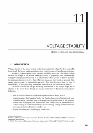
  • 4. 660 thus: V2 S2 = 1 2(R cos cp + X sin cp ± Z) VOLTAGE STABILITY 2Z[cos(,B - cp)± 1] (11.7) Because S2 > 0, the positive sign "+" at the nominator of equation (1 1.7) holds, therefore, the maximum loadability of the line: V2 S2max = 1 2Z[cos(,B - cp)+ 1] 4Z cos2[(,B - cp)j2] (11.7') thus resulting the same expression (8.6), previously computed following a different path (see Section 8.2.2), respectively: VI cos cp P2max = -:- 4Z =-- CO-S """ 2[ '-;- (,B -::---' _ '- cp ""7 ) ""7C j2 '"'" ] (11.8) 11.2.2 Load Modeling 11.2.2.1 Load Characteristics. Voltage stability, also known as "load stability," is strongly influenced by the static characteristics and the dynamic response of the load [1]. as: In the power systems terminology, the term "load" can have different meanings, such (i) a device connected to the power system that consumes active and/or reactive power; (ii) the total active and/or reactive power consumed by all devices connected to the power system; Asynchronous motors ("'T;����;�;i'��'�'����;k""'! ! (llOkV) I " ....____ ____•••__....__________ ---_____,1 f1Capacitor banks t-- .... Lighting Resistive loads Figure 1 1 . 1 . The load structure of a transm ission network bus.
  • 5. SYSTEM CHARACTERISTICS AND LOAD MODELING (iii) a part ofthe power system, which is not explicitly defined, but it is assigned as a device connected to the power system. The driving force for voltage instability is usually the loads. After a disturbance, load power restoration is attempted by motor slip adjustment, tap changing, and thermostats. Generally, the load modeling is an important issue, since in a power system the loads are aggregated, that is, they consist of different receivers. The main problem is the identification of the load components at a given instant and their mathematical represen­ tation. To understand the nature of the dependence between voltage stability and load dynamics, it is necessary to analyze the load in an individualistic approach. For this purpose, this section focuses on the dependence between voltage and load, especially on the properties of the exponential and polynomial load models. In power system stability studies, in general, and in voltage stability, in particular, the meaning of load is taken as the definition (iii), representing a distribution network that receives power from the transmission network through a substation. Therefore, the load connected to a bus, also known as complex load, includes, besides individual consumers (synchronous and asynchronous motors, resistive loads, etc.), the feeders, distributors, transformers, and so on (Figure 11.1). The load characteristics are a set ofparameters, such as the power factor or variation of active and reactive powers with voltage and frequency, that characterize the specific behavior of the load in static or dynamic states. The load mathematical model can be formulated in the general form as Ref. [3,51,52]: P = Kp . Po · fp(V,j) Q = KQ . Qo · fQ(V,j) (11.9) where Po, Qo are the active and reactive load powers, for values of voltage and frequency corresponding to the normal operating state (Vo,fo); Kp, KQ are the independent quantities, known as load demand coefficients; andfp,fQ are the functions expressing the dependency of the active and reactive load powers on the voltage and frequency at a given time. In steady state, the load characteristics, called static load characteristics, representthe dependency at a given time ofthe active andreactivepowers on the connection bus voltage and the system frequency in quasi-static state. This state is characterized by very slow modifications of the operating conditions, and the transition from one state to another can be considered a series of steady states (a series of equilibrium points). The modeling of these characteristics involves only algebraic equations. In dynamic state, the load characteristics, called dynamic load characteristics, also represent the dependency of the active and reactive powers on the connection bus voltage and the system frequency, but in transient state, when the operating conditions substantially changes from one instant of time to another. As general simplification, for voltage stability studies, the frequency dependency of the active and reactive powers is neglected, and therefore the general load mathematical model can be written as: P = Kp . Po ·fp(V) Q = KQ . Po ·fQ(V) (11.10) Unlike the system characteristics, where the amounts ofthe active and reactive powers that can be delivered to the load zone, the load characteristics define the variation of the 661
  • 6. 662 VOLTAGE STABILITY active and reactive powers in terms of the receiving-end voltage of the transmission line. For the considered configuration, this dependence can be written as: P2 = fp(V2, Po,2) Q2 = fQ(V2, Qo,2) (1 1.11) where P2 and Q2 represent the demanded powers under certain operating conditions. The last expressions define, in the (Vz, P2, Q2) space, a curve that, for a specific power demand, which does not exceed "the capability of the transmission network," intersects the surface defined by equation (11.5) in one or more points representing possible operating points. When the demand changes, these points move on the surface and their projection in the (V2, P2) plane represents the V2-P2 characteristic of the system (transmission network). Note that the system characteristic cannot be defined without specifying how the power delivered to the load varies. Therefore, the Vz-P2 characteristic corresponding to a constant power factor represents a particular case of system characteristic. 11.2.2.2 Static Models. EXPONENTIAL MODEL. This is one of the most used models, having the general form: (v)ap P = Kp' Po' Vo (l1.12a) (l1.12b) whereKp andKQare dimensionless load coefficients, being equal to 1 forthe base case; Vo is the reference voltage; and C¥p, c¥Q are the coefficients depending on the load type. The terms Kp. Po and KQ . Qo represent the absorbed active and reactive powers, respectively, at avoltageVequal tothereference voltageVo, andcorrespond tothenominal load powers. It is necessary to make distinction between the actually consumed power andthe load demand. This distinction is important for understanding the basic instability mechanism, since as the load demand increases theconsumedpowermay decrease, as a consequence of the voltage decrease. Three particular cases for C¥p and c¥Q are usually considered as follows: • constant impedance load: C¥p = c¥Q = 2 • constant current load: C¥p = c¥Q = 1 • constant power load: C¥p = c¥Q = 0 For lower voltage values the exponential model is not sufficiently precise, because, when the voltage drops below a certain value (e.g., V :s; O.6p.u.), many consumers are disconnected or their characteristics are completely altered. Two of the most important properties of the exponential model are presented. (i) Toinitialize theexponentialmodel, any voltage level can be used as reference. To demonstrate this property Kp = 1 is considered, while the reference voltage Vo
  • 7. SYSTEM CHARACTERISTICS AND LOAD MODELING and the powers Po and Qo can be arbitrarily specified without changing the characteristic. Thus, for a voltage level VI, we have If Po is expressed from the last equation then replaced in (l 1.12a) results: (V)<XP P = P1• � Thus, Vowas replaced with VI and Powith P], and the new reference voltage becomes VI' (ii) The exponents ap and aQ used in the load exponential model determine the powers sensitivity to voltage change. ConsideringVo as reference voltage and Po the active power load corresponding to this voltage value, the power sensitivity to voltage change can be calculated as: dP (V)<XP-l dV = ap' Po' Vo Vo Evaluating the sensitivity for V = Vo obtain as follows: respectively dP/Po --- -a dV/Vo- p dQ/Qo ----a dV/Vo- Q (l1.13a) (11.13b) Therefore, the sensitivities have the same values irrespective of the voltage reference value. The expressions (equation l 1.13a,b) can be written as: IlV IlP = ap-Po Vo IlV IlQ = aQ-Qo Vo If the pervious equations are divided member by member, gives: IlP ap Po IlQ aQ Qo Giventhe relationship Q = p. tanrpiftanrp = tanrpo = ct.(tanrpo = (Qo/Po)) obtain as follows: meaning that for constant power factor, ap=aQ. POLYNOMIAL MODEL. Since different components of a complex load present different voltage characteristics, an alternative load model obtained by summing up the load 663
  • 8. 664 TAB L E 1 1 .1 . Polynomial Load Models (3) Load Type Air conditioner Asynchronous motors Complex load 0.83 - 0.3 (fo)+ 0.74 (fo)2 VOLTAGE STABILITY 2.08+ 1.63 fo - 7.6 (fo)2 + 4.89 (for 6.7 - 15.3 (fo)+ 9.6 (for components, which presents the same (or almost the same) exponent, should be considered. When all exponents are integers, the load characteristic becomes a polynomial function of V. A special case is the load model consisting ofthree components: constant impedance, constant current, and constant power. In this case, the characteristics of the active and reactive power, respectively, of the load model are given by the expression [2]: P = Kp. po· [ap. (:J2 + bp .:0+ cp] Q = KQ. Qo· [aQ . (:J2 + bQ .:0+ CQ] (1 1.14) where ap, bp, Cp, aQ , bQ, cQ represent the weights of each component and satisfy the relationships ap + bp + Cp = 1 and aQ + bQ + cQ = 1; and Kp. Po, KQ. Qo are active and reactive consumed powers, corresponding to the reference voltage Vo. Similar to the exponential model, for reduced voltage values, the polynomial model cannot be used to appropriately model the loads. Table 1 1.1 shows some polynomial models [3]. 11.2.2.3 Dynamic Models. These models describe, through algebraic-differential equations, the dynamic behavior of the load given either by the intrinsic load character­ istics orby the actions ofsome control devices such as the automatic on-load tap changer or the thermostat load control systems. Because the use of physical dynamic models specific to some loads, such as large synchronous and asynchronous motors individually represented, is inadequate forcomplex load modeling, the so-called generic dynamic models have been developed. They describe the specific behavior of the complex load when subjected to sudden voltage variations in the connecting node, due to various disturbances occurring in the transmission network. The measurements at the HV bus bars of some substations supplying the distribution network showed that the response of the complex load to sudden voltage variations is as illustrated inFigure 11.2 fora real power P [4]. This response reflects the collective effects of all the complex load components, from the on-load tap changer to the individual household loads (Figure 1 1.1). The time span for a load to recover to steady state is
  • 9. SYSTEM CHARACTERISTICS AND LOAD MODELING (a) V (b) P Po P, - - - - - - t-------;-:--::�� -- ' P.,o Figure 1 1 ,2, The dynamic active power response of a complex load (b) at sudden voltage variation in the connection node (a) [4], normally in the range of several seconds to minutes, depending on the load composition, Responses for real and reactive power are qualitatively similar. It is obvious that a sudden voltage variation determines an instantaneous change in the consumed power. This variation defines the transient characteristic o/the load and can be modeled as constant impedance �n as used in the transient stability analysis tools, or, more general, as an exponential characteristic. A dynamic load restoration process follows characterized by an increase in the power demand up to a new voltagevalue on the steady­ state characteristic. On a longer timescale, the lower voltage tap changers and other control devices act to restore voltages and so the load. In fact, the aggregate effect ofdistribution-Ievel restoration can be to cause load overshoot. With recovery time (Tp) on a timescale of a few seconds, this behavior captures the behavior of induction machines. On a timescale of minutes, the role oftap changes and other control devices is included. Over hours, the load recovery and possible overshoot may emanate from heating load [4]. The dynamic restoration process can be asymptotic or even oscillatory (Figure 1 1.2b) and can be modeled through a set of differential equations [2]: (11.15) where Po, Qo are the active and reactive consumed powers in normal operating state characterized by the voltageVo; Ps, Pt are the steady-state and transient load characteristics of the active power; Qs, Qt are the steady-state and transient load characteristics of the reactive power; Xp, XQ are the generic dimensionless state variables associated with the load restoration dynamic process; and Tp, TQ are the load restoration dynamic process. The generic models are usually associated with the exponential load models. Hence, the steady-state characteristic is given by expressions (1 1.12) where Kp = KQ = 1: (V )ap Ps = Po' Vo ; (1 1.12') Depending on the way in which the generic variables Xp and XQ intervene in the expressions of the transient load characteristics, there are two types of generic dynamic 665
  • 10. 666 VOLTAGE STABILITY models: the additive model where the generic state variables are appended to the transient characteristic and the multiplicative model where the generic state variables multiply the transient characteristics. (i) The additive generic model The transient load characteristic is given by [2]: (1 1.16) where Q'P,I and Q'Q,I are exponents of the transient load characteristics. Hence, the differential system of equations (11.15) describing the load restoration dynamic process becomes: dXp 1 (V)<XP (V)<XP" Tp-=-(Ps -PI) = - - - -Xp dt Po Vo Vo dXQ 1 (V)<XQ (V)<XQ,' TQ-=-(Qs -QI) = - - - -XQ dt Qo Vo Vo (ii) The multiplicative generic model The transient load characteristic is given by: PI =Xp .Po' (V/Vo)"P" (1 1.17) (1 1.16') and the differential system of equations (11.15) describing the load restoration dynamic process becomes: Tp dXp =�(Ps -PI) =(V/Vo)"P -Xp .(V/Vo)""" dt Po TQ dXQ =�(Qs -Qt) = (V/Vo)"Q -XQ . (V/Vo)"Q,' dt Qo (1 1.17') The following remarks are made regarding the two generic dynamic models [2]: (i) the exponents Q'P,t and Q'Q,t have usually large values and thus the dependence on voltage of the load powers is greater in transient state than in steady state; (ii) the generic state variablesXpandXQ must range within acceptable limits, that is: Xwin :s Xp :s XWax XQin :S XQ :S XQax (1 1.18) (iii) the constant power type component introduced in the additive models may cause nonphysical singularities to the transient characteristic, which is not the case for the multiplicative model;
  • 11. STATIC ASPECTS OF VOLTAGE STABILITY (iv) the simple model given in(I1.12') can be obtained ifwe take Xp = XQ = O in the additive model, and Xp = XQ = 1 in the multiplicative model, respectively; (v) the exponents Q'p and Q'Q and the time constants Tp and TQ can be determined using measurements of powers supplied to the distribution network either considering disconnection of a transformer or on-load tap changing in the HVIMV distribution substation leading to gradual modification of the voltage level Ref. [2]. 11.3 STATIC ASPECTS OF VOLTAGE STABILITY 11.3.1 Existence of Steady-State Solutions The projection of the points corresponding to the maximum transmissible power S2max in the (P2, Q2) plan determines a curve that separates the plan into two zones (see Figure 1 l .3) [5]: The hatched zone represents the domain of existence of solutions and corresponds to the possible operating points (A and B in Figure 11.4), for which the biquadratic equation (11.3) has two distinct real positive solutions. Using the notations: y = V� Q' = vf - 2(RP2 + XQ2) Ii = [2(RP2 + XQ2) - Vf] 2 - 4Z2(p� + QD from (1 1.3) a quadratic equation in y is obtained as follows: v, 0, Geometrical locus of the critical points of the solutions (1l.3) (1l.l9) Figure 1 1 .3 . The dependence between the voltage V2 and the powers P2 and Q2< for a simple generator-li ne-load config u ration. 667
  • 12. 668 v, � Controllable zone VOLTAGE STABILITY �,max 1-----.:;:",.___ : A Security zone Critical �,m in I----------!---..::...... / point Critical zone v"cc '-----------!------. , I.C ;;; I' I • I • " . " . .�......... � ;; : B : ;;; � �---T------�--� Uncontrollable zone P, P2mo> Figure 1 1 .4. The VrP2 system characteristic: operating poi nts, with the solutions Yl,2' which give the voltages corresponding to the two possible operating points A and B: v - Ja+ JI5., 2A - 2 ' V2B = Ja- JI5. 2 (11.20a,b) • The external zone represents the domain of inexistence of solutions, thus no operating points are found in this area. • The critical points situated on thefrontier represent static bifurcation points for the system evolution as they are characterized by zero value of the discriminant from equation (11.19), Ll = 0, of the biquadratic equation (11.3), resulting: If Ll = 0 is considered in the expressions (11.20a and b), identical solutions V2A and V2B are obtained in the critical points, corresponding to the possible operating points: VI - 2(RP2max +XQ2max) 2 (1 1.21) Note that in the critical points situated on the separation frontier of the domain of existence of solutions in the P2-Q2 plan, the Jacobian matrix of the Newton-Rhapson method-based loadflow mathematical model become singular. We know that: 11 Pi = GuV7 + LViVkGGik k=l keFi OPi 2 � 2 2 � 2 oVi Vi = 2GUVi + � VYkGGik = GUVi + GUVi + � ViVkGGik = GUVi +Pi k=l k=l
  • 13. STATIC ASPECTS OF VOLTAGE STABILITY 669 where OPi Pi + GiiV? oVi Vi n Qi = -BuV? - LVYkBBik k=1 k#i OQi 2 ...f- 2 oVi Vi = -2BuVi - � VYkBBik = -BUVi +Qi k=1 k#i OQi Qi - BiiVf oVi Vi The Jacobian matrix of the power system from Figure 7.1, considering that the bus 1 (the slack bus) voltage is taken as phase reference with Y1 = VI lei = 0 , and the bus 2 voltage is Y2 = V2 lti2 ' has the following form: where OP2 _ P2 + G22V�. oV2 V2 ' Thus, the determinant of the Jacobian matrix is
  • 14. 670 Because in the critical point vi = vier = Z2 .S�, it results: det[i] = 0 VOLTAGE STABILITY This property, valid for a simple generator-line-load configuration as well as for any complex network, is the core of voltage instability and collapse risk assessment, due to the inexistence of the equilibrium points (steady-state solutions) caused by load increase and/or due to the contraction of the domain of existence of the solutions after a contingency. 11.3.2 Operating Points and Zones For analysis ofthe points inside the hatched zone (Figure 1 1.3), the dependence between P2 and Q2 through the power factor cosrpis considered. Thus, equation (11.4) can be written as: vi + [2P2(R + Xtanrp) -vf] V� + Z2 (�) 2 = 0 cosrp (1 1.22) If VI and cosrp are considered constant, then for values of the active power P2 E [0, P2max], an expression ofthe form V2 = f(P2), called the V2-P2 "system character­ istic," can be obtained (see Figure 11.4) [5]. Figure 11.4 shows that for a transmitted power P2 ::; P2max, two possible operating points are found as: point A, characterized by a high-voltage value, corresponds to the normal operating conditions being a stable operating point, whereas point B, characterized by a low-voltage value, corresponds to abnormal operating conditions. To demonstrate why A is stable and B is unstable, the effects of voltage regulation by the control ofthe power factor at the transmission line receiving end and voltage variation at the transmission line sending-end will be analyzed. v, (i) The effect of compensating the transmitted reactive power Considering different values for cosrp and keeping constant the sending-end voltage of the transmission line (VI = ct.), the family of V2-P2 characteristics from Figure 11.5 is obtained. For a given value P2 < P2max, the V2A voltage corresponding to the operating point A increases as the power factorchanges from inductive to capacitive values. Atthe same time, inthe point B, compensation ofthe reactive power has opposite cos cp = 0.95 lag cos cp = 1.0 � r-o:::::::::I=:::t:::-f-- cos cp = 0.95 lead power factor v cap 2,cr V ind 2,cr P, Locus of critical points P, Figure 1 1 . 5. Effect of reactive power com­ pensation on the VrP2 characteristic.
  • 15. STATIC ASPECTS OF VOLTAGE STABILITY q, 1 0.75 T 0.50 0.25 effects since the voltage decreases as cos cp changes from inductive to capacitive values. Therefore, point A is a controllable operating point and thus stable; whereas point B is uncontrollable and thus unstable. The locus of critical operating points is shown by dotted line in Figure 11.5. Normally, only the operating points above the critical points represent satisfac­ tory operating conditions. Thus, a sudden reduction in the power factor (increase in Q2) can cause the system to change from stable operating conditions to unsatisfactory, and possibly unstable, operating conditions represented by the lower part of a V2-P2 curve. The influence of the reactive power characteristics of the equipments at the receiving end (loads and compensating devices) is more obvious in Figure 11.6 [6], which shows a family of curves applicable to the power system from Figure 1 1 .4, each of which representing the relationship between V2 and Q2 for a fixed value of P2. For a complex system, these curves can be obtained for a load bus through repeated load flow calculations. In this regard, consider that a virtual reactive power source (without power limits) is connected to the bus. As a consequence, thisbusbecomes aPVbus where the voltage is imposed and the reactive power is calculated. An example of this type of characteristics, in p.u., q = QX/V�, is given in Figure 11.6 for a transmission line (X » R) having an active source as parameter (p = PX/VT) and a switched capacitor bank. The system is stable in the region where the derivative dQ2/dV2 is positive. The voltage stability limit (critical operating point) is reached when the deriva­ tive is zero. Thus, the zones on the Q2-U2 curves to the right of the minima represent stable operation, and the zones to the left represent unstable operation. Stable operation in the region where dQ2/dV2 is negative can be achieved only with a continuously regulated reactive power equipment that has sufficient control range and high QIV gain with polarity opposite to that of the normal. If no capacitor bank is connected, the operating point is at the intersection of the V-Q characteristic with the horizontal axis (Figure 11.6, the a curve). If reactive power compensation is provided, a new operating point can be found at the intersection between the bus characteristic and the capacitor bank character­ istic (Figure 11.6, curves b and d). Notice that for large values of the transferred active powers, if there is insufficient compensation, no operation point can be defined. Operating point Operating point O�������-.--+� ' Reserve in MVAr without capacitor (case ) -0.25 --"":------'--- Figure 1 1 .6. The Qru2 cu rves for vari­ ous real-power load [6, 51). 671
  • 16. 672 VOLTAGE STABILITY V, The reactive power reserve to maintain normal operation is the distance, in MVAr, from the operating point to the minimum ofthe bus characteristic (Figure 11.6, case 1), without capacitor, or to a point where the capacitor bank characteristic on the lowest step is tangent to the bus characteristic (Figure 11.6, case 2). The slope ofthe characteristic in the operating point is the aQ/aV sensitivity that shows the robustness or weakness of the analyzed bus as well as the effectiveness of reactive power compensation. (ii) The effect of controlling the transmission line sending-end voltage Considering different values for the transmission line sending-end voltage, Vii) and V(2), obtained by modifying the generator's field current, and constant powerfactor (cos c:p = ct.), thefamilyof V2-P2 characteristics from Figure 11.7 is obtained. In this case, for a constant value P2 < P2max of the transmitted active power, the point A is a normal operating point because the corresponding voltage (VA) increases as the transmission line sending-end voltage increases. In exchange, the point B is an abnormal operating pointbecause the sending-end voltage increases as the voltage corresponding to this point decreases. Therefore, the control of VI voltage at the transmission line sending­ end through change of the generator's field excitation current has the desired effect on the operating point A, while for the operating point B the effect is opposite. Moreover, analyzing the characteristics from Figures 1 1.5 and 11.7, we can see that the critical voltage and the maximum transmissible power increase as the reactive power is compensated with the help ofreactive power devices, or as the transmission line sending-end voltage increases. When operating near the limit, the two voltages corresponding to the possible operating points will have high and closed values. Therefore, the voltage attached to one operating point only is not an indicator of voltage instability proximity. Additional information such as voltage sensitivities to active and reactive powers variation is thus necessary. (iii) Voltage sensitivities to active and reactive powers variation The voltage sensitivities can be obtained by differentiating equations (11.4). To simplify the calculus, a small phase difference between the voltage phasors at the transmission line ends is assumed, that is, 8 = (81 - 82) � O. Therefore, using equations (1 1.2a) and (11.2b), since cos 8 � 1 and sin8 � 0, equation (1 1.3) becomes: 11,') r----l-<'---- 0') 1 11,(1) r-_-'- """"__--'-___'cc-_--,'::-+ P, Figure 1 1 .7 . The effect of controlling the voltage V, P, on the VrP2 characteristic.
  • 17. STATIC ASPECTS OF VOLTAGE STABILITY The voltages corresponding to the possible operating points A and B are as follows: VI + VVI -4(RP2 +XQ2) V2A � -- --'----- ----:,-------- 2 (l1.23a) VI - VVI -4(RP2 +XQ2) V2B � ----'------:,-------- 2 (1 1.23b) A power system, seen from a bus i, is stable from the viewpoint of the bus voltage, if the addition of a conductance aGi or a susceptance aBi, respectively, eventually infinitesimal, determines the increase in the consumed active and reactive powers, and a simultaneous decrease in the voltage of the considered bus. Therefore, the necessary and sufficient condition for the power system to be controllable is [7] - <0' dVi I dGi Bi=ct ' dVi I 0 - < . dBi Gi=ct ' - > dPi I 0 dGi Bi=ct - > dQi I 0 dBi Gi=ct (11.24) The sensitivities 2 ofvoltage tothe activeandreactive powers intheA and B points can be calculated starting from the expressions (11.23a,b): -4R -R 2 · 2VVT -4(RP2 +XQ2) -----r====== <0 VVT -4(RP2 +XQ2) 8V2A I -x 8Q2 PFct = VVT _ 4(RP2 +XQ2) <0 R -----,=-====== > 0 VVT -4(RP2 +XQ2) 2 If y = VuW then y ' = � or <!l = � 2�' du 2� (l1.2Sa) (1 1.2Sb) (l1.2Sc) (l 1.2Sd) 673
  • 18. 674 VOLTAGE STABILITY According to the definitions from (1 1.24) and (1 1.25), point A is a controlla­ ble operating point, thus stable, and point B is an uncontrollable operating point, thus unstable. Considering these aspects, the following operating zones can be defined on the V2-P2 characteristic (Figure 11.4): • The Controllable Zone. Corresponds to the upper side of the characteristic and comprises the operating points forwhich Zc > Zand sensitivities are negative. In the technical literature, this zone is known as the stable operating zone. If the critical voltage is lower than the minimum admissible operating voltage (Vmin), this zone can be divided into two subzones: - The Security Zone. Defined between the maximum and the minimum admissible voltages (Vmin and Vmax), characterized by negative and close to zero sensitivities; - The Critical Zone. Defined between Vmin and Vcr voltages, characterized also by negative sensitivities but high in magnitude. Depending on the load characteristic, operation in this zone can trigger voltage instability phenomenon or voltage avalanche, phenomenon characterized by a voltage decrease towardVcr. either due to an increase in the power demand or due to the on-load tap changing transform­ ers action. • The Uncontrollable Zone. Corresponds to the lower side of the characteristic and comprises the operating points characterized by Zc < Z and positive sensitivities. This zone is known in the technical literature as the unstable operating zone. Note that the assumption of a small phase difference (e small) is no longer possible to determine the critical voltage because, if in equations (1 1.23a,b) the zero condition of the discriminant would be imposed, the critical voltage is obtained Veri! = VJ/2, value that depends on the sending-end voltage but is independent of the power factor, which is in contradiction with the remark previously made. 11.4 VOLTAGE INSTABILITY MECHANISMS: INTERACTION BETWEEN ELECTRICAL NETWORK, LOADS, AND CONTROL DEVICES In power systems operation, the maximum transmissible power and the critical voltage are only for theoretical importance since they cannot be precisely determined due to the phenomenon complexity, depending on a series of factors influencing each other (load behavior, keeping the voltage to the reference value in the generator nodes, the reactive power compensation devices action, etc.). 11.4.1 Interaction between Electrical Network and Load There are two basic mechanisms that can lead to voltage instability and collapse phenomena in power systems. One of these mechanisms is the slow increase in the load demand, and the other one resides in the disturbance occurrence in the transmission network (disconnection of electrical lines, transformers, generators, etc.) that lead to the modification of the V2-P2 characteristic.
  • 19. VOLTAGE INSTABILITY MECHANISMS: INTERACTION BETWEEN ELECTRICAL NETWORK (a) V, Load increase V,r-_-J B (b) V, Load increase � r--_� . P, P2,m ax - Figure 1 1 .8. Voltage instabil ity mechan ism i n terms of load demand i ncrease: (a) P= ct; (b) voltage-dependent load. (i) The voltage instability phenomenon mechanism, caused by the load increase, considering different static load characteristics, is illustrated in Figure 1 1.8. • Thus, for a P= ct. load characteristic, as the demand power increases, due to the load characteristic shifting, the two equilibrium points approach each other, overlap in the critical point C (which represents a singular point coinciding, in this case, with the maximum transmissible power) and then disappear (Figure 11.8a); • Ifthe load is representedby exponential model, and the operating point is situated on the upper side, as the load demand increases, this point moves from AI to A2 (Figure 1 1.8b) leading to voltage decrease simultaneously with increase in the transmitted power, which corresponds to a normal operation ofthe "transmission network-load" configuration. Instead, if the operating point is situated on the lower side, as load demand increases, the point moves from B1 to B2 causing a decrease both in the voltage level and in the transmitted power, which corresponds to an abnormal operation of the transmission network-load configuration. (ii) The voltage instability mechanism to a major disturbance, caused by dis­ connection of one circuit of the transmission line, is shown in Figure 11.9. The disturbance occurrence causes inthe first moments a decrease involtage and therefore sudden decrease in the load demand, in accordance with the transient load characteristic, and the operating point moves from Al, situated on the normal operation characteristic, to A2, situated on the postdisturbance charac­ teristic. As the transient process evolves, the point A2 moves toward a new equilibrium point, given by the intersection between the static load characteristic and the postdisturbance characteristic ofthe transmission network. We see that, if the load is of P= ct. type there is no intersection point between the two characteristics, which determines the voltage to collapse at the load terminals (Figure 1 1.9a). Instead, if the load is represented by exponential model, the two characteristics intersect in point A', which is the new operating point characterized by a reduced voltage level (Figure 1 1 .9b-curve a) (see also Section 8.2.2). However, in this case, the voltage collapse can be triggered by the on-load tap changer actions, trying to restore the voltage to the reference value. The consequences of this action are the change of the load characteristic seen from the transformer primary and the increase in the consumed power from the system, which increase the risk for voltage instability and voltage collapse (Figure 1 1 .9b-curve b). 675
  • 20. 676 (a) V, Postdisturbance Predisturbance characteristic characteristic �=-------�---.� (c) 0.0 (b) B Po VOLTAGE STABILITY Postdisturbance v, characteristic Predisturbance """"=-------�---. P, Postdisturbance system curve C 1.0 P Figure 1 1 .9. The voltage instabil ity mechan ism to major d istu rbances (a and b) and the reg ion of attraction (c). These mechanisms caused by the load behavior are strongly influenced by the on-load tap changer action, a reactive power deficit due to limitations in the generator's field and armature currents, as well as following the secondary voltage control system actions. The portion of the V-P characteristic that allows restoring the system operation to a stable equilibrium point is called region of attraction (Figure Il.9c). Consider the simplified radial power system with constant sending-end bus voltage and unity power factor load. As shown before, there are two possible equilibrium points corresponding to Po = ct: point A situated on the upper section of the V-P curve, which is a stable equilibriumpoint, and point B situated on the lower section ofthe V-P curve, which is an unstable equilibrium point (Figure Il.9c).1t can be shown that, after a disturbance, ifthe power system reaches an operating point situated anywhere on the DACB section of the V-P characteristic, appropriate measure can help increasing the voltage and thus moving the system operation in a stable equilibrium point corresponding to the demanded power. [8,9]. 11.4.2 Influence of the On-Load Tap Changer In some power system operating conditions, the on-load tap changer actions performed under an automatic voltage regulator (AVR) may enhance the risk for or even trigger the voltage instability process [10]. To analyze this phenomenon, let us consider the one-line diagram fromFigureII.lOa ofa system supplying through a shortelectrical line and an on­ load tap changing (OLTC) transformer equipped with AVR. 11.4.2.1 Modeling the On-Load Tap Changing Dynamics. Neglecting the transformer no-load losses, including its series impedance in the equivalent impedance � and modeling the load by the impedance �c, the equivalent circuit from Figure Il.lOb is obtained.
  • 21. VOLTAGE INSTABILITY MECHANISMS: INTERACTION BETWEEN ELECTRICAL NETWORK (a) P,+jQ, Figure 1 1 . 1 0. One-l ine d iagram (a) and equ iva lent circu it (b) for the analysis of the on-load tap chang ing influence. The turns ratio N is a real number given by: (11.26) where Vnp is theprimary winding nominal voltage (the nominal voltage ofthehigh-voltage winding, equipped with tap changer); Vns is the secondary winding nominal voltage; np is the actual tap position (actual operating tap); and LlVp is the percentage ofvoltage variation per tap (expressed in percents). The turns ratio N varies within the admissible interval [Nlo, Nup] given by the transformer's control capability (number of taps). The role of AVR is to change on-load the ratio N so that the load side voltage V2 is kept inside the interval [V2,sch - 8, V2,sch + 8], called the insensitivity domain of the regulator, around the reference voltage V2,sch, determined under stable-operating conditions. Therefore, if the load side voltage is lower than V2,sch - 8 then, after a period called delay period, according to expression (11.26), written as V2 = V2'/N, the regulator will command the tap change with one position in the sense of turns ratio decrease, resulting the increase of V2. Reverse, if V2 > V2,sch + 8 the regulator will command the tap movement with one position in the sense of turns ratio increase, resulting the decrease of V2, The process will continue until either the voltage is brought back within the admissible interval or one of the limits, Nlo or Nup, is reached (the tap changer reaches one of its extreme positions). The dynamic behavior ofan on-load tap changing transformer equipped with AVR can be described using either a discreet model or a continuous model. • The discrete model assumes that the regulator, activated whenever the load side voltage does not fulfill the condition IV2 - V2,sch I :::; 8, will command the tap change at discrete time intervals tko k = 0, 1, . . . , n, which satisfies the recursive formula: tHI = tk + LlTk and to = O. In this expression, LlTk denotes the time delay and depends on the regulator characteristics and the voltage error, Generally, LlTk is not necessarily constant and may be determined using the expression [2]: 8 LlTk = Td I I + Tf + Tm V2 - V2,sch (11.27) where Td is the maximum time delay of the inverse time characteristic; Tf is a fixed value ofthe time delay; T.n is the mechanical time necessary to perform the tap change; and E is half of the OLTC deadband, 677
  • 22. 678 VOLTAGE STABILITY The tap changing logic, called direct or normal logic, can be defined as: V2 < V2sch - 8 and Nk > Nlo IV2 - V2schI :s; 8 V2 > V2sch + 8 and Nk < Nup (1 1.28) where � is the size of tap step and Nup, N,o are the upper and lower tap limits. • The continuous model assumes a continuous variation of the turns ratio N(t) within the interval [N,o, Nup] and ignores the insensitivity domain of the regulator. Therefore, the tap changer dynamics can be modeled through the following differential equation: dN 1 - = --(V2 - V2sch) dt TAVR where TAVR is the time constant of the regulator. (1 1.29) Although the continuous model is less accurate than the discrete model, it is more frequently used in the technical literature because it allows the analytical investigation of the tap changing behavior and highlights the influence on the voltage stability [2]. 11.4.2.2 The Effect ofAutomatic Tap Changing on the Possible Operating Points. It was demonstrated in Section 7.2.3.4 that the static characteristic V2 = f(N) of an on-load tap changing transformer can be obtained by using expression (7.26), as the curve shown in Figure 7.17: NV,Rc ( / V2 = f(N) = - X - 1 The maximum load side voltage, V2max, (7.31) can be obtained for a turns ratio Nmax (7.30): Nmax = fX V R: (7.30) (R; V2max = V' V iY (7.31) The equilibriumpoints definedby condition dN/dt = 0 are obtainedby intersecting the characteristic V2 =feN) defined by expression (7.26) with the horizontal line ofV2 =V2,sch (Figure 7.17). Analysis ofFigures 7.17 or 11.11 reveals that for a scheduled valueV2,sch< V2,maxtwo operating points, A and B, are found, whereas for V2,sch>V2,max no operating point is possible. This shows that no value ofthe load side voltageV2,schcan be reached through on­ load tap changing and turns ratio control. In order to determine the nature of the equilibrium points A and B, a virtual disturbance is assumed, such as an incremental change LlV2,schof the load side scheduled voltageV2,sch(Figure 11.11), then the resulted transient state is analyzed. According to the
  • 23. VOLTAGE INSTABILITY MECHANISMS: INTERACTION BETWEEN ELECTRICAL NETWORK V, �,max --------- f-�-__!_-----l_:_:_- V2."h+D.1I,."h t--+- - -+- - - _____ ,--- �,sch Figure 1 1 . 1 1 . The effect of the on-load tap chang ing reg u l ation on the possible operating poi nts A and B. normal control logic, the regulator will command the turns ratio to decrease so that V2 increases to the new reference value V2•sch + LlV2•sch' It is obvious that, if the operating point is A, the turns ratio decrease will result in the movement ofthis point toward the new equilibrium point AI demonstrating thatpoint A is a stable operating point. Instead, point B is an unstable point since a turns ratio decrease will cause movement away of the new equilibrium point B/. Therefore, the stable operation of the transformer's AVR corresponds to the points on the static characteristic located on the right side of Nmax, characterized by negative values of the derivative V2/dN. Instead, for the points located on the left side of the Nmax value, characterized by V2/dN> 0, the AVR operation is unstable. 11.4.2.3 Influence ofOn-Load Tap Changing on the Voltage Stability [18]. In order to establish the conditions under which the on-load tap changer actions can cause voltage instability, on one hand, the V2 =feN) curves are analyzed in two situations influenced by various factors among which the sending-end voltage VI and the load power, and, on the other hand, the tap changer behavior in the possible operating points on the V2-P2 system characteristic. In this regard, assumes that the static characteristic from (7.26) is expressed in p.u., hence the nominal turns ratio is Nnom = 1. v, (i) The Constant Load Case (R e = ct.). For different values of the voltage VI, the maximum point ofthe V2 =feN) characteristic does not change (Nmax = JX /R c remains constant!), while the maximum value of the receiving-end voltage, V2max = VI JR c/2X , decreases simultaneously with VI (Figure 11.12). Thus, as the VI voltage decreases, the equilibrium points A and B move closer to each other, overlap in the maximum point-which constitutes a static bifurcation point, then disappear. When the equilibrium points disappear, the tap changer dynamic behavior becomes unstable and, in its attempt to reach a new operating point, the AVR causes the voltage collapse phenomenon. L---�� � -�---+N N max Figure 1 1 . 1 2 . The evol ution of the V2 = f(N) static characteristic with the send ing-end voltage V1 • 679
  • 24. 680 V2 VOLTAGE STABILITY F i g u re 1 1 . 1 3 . The evol ution of the V2 = f(N) static characteristics with the load . (ii) The Constant Source Voltage Case (VI = ct.). If the load increases from p�l) to p�2) andfurtherto p�3), that is, the load resistance decreases (R�3) < R�2) < R�l)), then the maximum point Nmax = JX /Re ofthe static characteristic moves to the right (Figure 1 1.13) since: (3) _ IT (2) _ IT (I) _ IT Nmax - VR�3) > Nmax - VR�2) > Nmax - VR�l) while, according to equation (7.31), the maximum receiving-end voltage decreases: (I) _ � JR�I) (2) _ � JR�2) (3) _ � JR�3) V2max - v'2 X > V2max - v'2 X > V2max - v'2 X Also in this case a load increase (p(I) < p(2) < p(3) or R(I) > R(2) > R(3) , 2 2 2 e e e ' respectively) determines the two operating points, A and B, to move closer to each other then to disappear in a static bifurcation point triggering the voltage collapse phenomenon. The most severe situation appears when, during operation, the sending-end voltage decreases while the load increases simultaneously. Therefore, paradoxi­ cally, an AVR controlled transformer, in its action to keep the voltage constant, may cause the voltage collapse phenomenon! (iii) TheBehaviorofthe On-LoadTap Changer in the TwoPossible OperatingPoints of the VrP2 System Characteristic. In order to analyze the tap changer behavior in the two possible operating points on the system characteristic, assumes that, for some reasons (the transmitted power P2 increases, the sending-end voltage VI decrease, etc.), the load side voltage has decreased below V2•sch- 8. Under this assumption, inaccordingwith thenormalcontrol logic, afteratime delay the AVR will initiate the turns ratio decreasing in order to restore the load side voltage. For the operating point A, situated on the upper side of the V2-P2 characteristic specific for Re > X (Figure 11.14a), the automatic tap changing system has a stable behavior. Indeed, from Figure 11.14b, it can be "seen" that, for instance, as the load increases (Re decreases), the operating point, situated at theintersectionbetween theV2 =f (N) characteristic, which corresponds to R�l), and the horizontal line V2 =V2•sch, moves in the point situated on the V2 =feN) characteristic, which corresponds to R�2) . Therefore, as
  • 25. VOLTAGE INSTABILITY MECHANISMS: INTERACTION BETWEEN ELECTRICAL NETWORK (a) II, �----��----�---+ � Rc<X (b) II, (c) II, Figure 1 1 . 1 4. The behavior of the on-load tap changer i n the two possible operating poi nts. the turns ratio decreases, the point moves on the new characteristic toward the final operating point, which corresponds to V2 =V2,sch' For the operating point B, situated on the lower side oftheV2-P2 characteristic (Figure 11.14a) specific forRc < X, the AVR action is destabilizing. Indeed, from Figure 11.14c, it can be seen that, as the turns ratio N decreases, the operating point moves away from the new equilibrium point and the load side voltage decreases. This process will continue until the ratio reaches its lower limit Nlo or until the voltage collapses. From physical viewpoint, when the load side voltage decreases, the tap changer acts to restore the voltage to its reference value. For this purpose, the AVR initiates the turns ratio decreasing no matter if Rc is higher or lower than X. Following this action, the load impedance value seen from the transformer primary decreases, and the primary current increases while additional voltage drop occurs. Consequently, the secondary voltage evolution is given, on one hand, by an increase caused by the control of the transformer ratio, and, on the other hand, a decrease caused by decrease in the primary voltage. Therefore: • for Rc > X, the first effect is dominant and the load side voltage is restored to the specified value; • for Rc < X, the second effect is dominant and the tap changing action cannot longer compensate the decrease in the secondary voltage but, on the contrary, it will accentuate the phenomenon of voltage decrease. From the above analysis, it is obvious that the operating point must be situated on the upper side oftheV2-P2 system characteristic. On this side, the tap changer can compensate the voltage fluctuations caused by changes in power flows or by disturbances that could modify the values of Zor VI' For this reason, the points situated on the upper side of the V2-P2 characteristic are considered to be stable operating points and the ones situated on the lower side are considered to be unstable operating points. Also, the turns ratio changing action indirectly restores the load power. 681
  • 26. 682 2 P3+J:j �1(" j1(, d,�� Transmission On-load tap changing network transformer Load VOLTAGE STABILITY Figure 1 1 . 1 5. The eq u ivalent circu it for analysis of load restoration th roug h auto­ matic on-load tap chang ing actions. The load restoration process through the automatic tap changing actions and its impact on the voltage stability can be analyzed, considering again the simple radial network from Figure l1.lOa and b. In this case, however, the transformer is explicitly modeledthroughits parameters referredto the medium voltage, being assignedto the load area. Thus, to analyze the interaction between the transmissionnetworkand the load, it is necessary to trace the load characteristic seen from the transformer primary. For simplicity, the resistances and the shunt parameters are neglected resulting the equivalent diagram from Figure 11.15. Furthermore, consider that the load connected to bus 2 has a voltage-dependent characteristic, that is: Ifthe voltage Y2 is taken as phase reference, from the equivalent circuit itresults that: and (1 1.30) However, the active and reactive powers entering the transformer from the transmis­ sion network depend on the secondary voltage V2: P3 = P2 =!P(V2) P� + Q� Q3 = Q2 + Xr V2 =!Q(V2) 2 (1 1.31) Using equation (1 1.30), P3 and Q3 can be expressed in terms of the V3/N ratio: (1 1.31') which, for a given turns ratio valueN, they may represent the transient load characteristics seen from the transformer primary. When the transformer is equipped with AVR aiming to maintain the voltage at bus 2 at a scheduled value V2,sch, the load active and reactive powers are constant and given by equations (11.31) by replacing V2 with V2,sch' These powers do not depend on the
  • 27. VOLTAGE INSTABILITY MECHANISMS: INTERACTION BETWEEN ELECTRICAL NETWORK (b) II, a r--===;:::::-� P3 P3 Figure 1 1 . 1 6. The load restoration process fol l owing the on-load tap chang ing action: (a) stable case; (b) unstable case. transmission line receiving-end voltage V3 andthereforethe static characteristic ofthe load "seen" from the transformer primary is of constant power type. In normal operating conditions, the operating point Ao is situated at the intersection between the system characteristic (Figure 11.16 a, curve a) and the load characteristic. When a disturbance occurs in the transmission network (for instance, disconnection of one transmission line circuit), the operating point, characterized by the voltage V2,sch, moves in the point A situated at the intersection between the postdisturbance characteristic of the system (Figure 1 1.16 a, curve b) and the transient load characteristic that corresponds to the actual turns ratio No. Note that, in the new operating point, which is a short-term equilibrium point, the consumed power P2(V2) is smaller than the power consumed in the point Ao and V2 < V2,sch since the turns ratio did not change. If the voltage is no longer within the admissible limits, that is, V2 < V2,sch - 8, the OLTC will start changing the tap in the sense ofvoltage V2 increase. The operating point moves on the postdisturbance characteristic, in accord­ ance with the new transient load characteristics (corresponding to the new turns ratio values), until V2 returns inside the admissible band V2,sch - 8 :s; V2 :s; V2,sch + 8. A new operating point D is, therefore, obtained at the intersection between the static load characteristic and the postdisturbance system characteristic. However, although the load voltage (the secondary transformer voltage) is restored, the transmission line receiving-end voltage is lower in comparison with the case in which the transformer would have been equipped with AVR (Figure 1 1.16 a, point A). Depending on the loading degree and the gravity of disturbance occurred within the transmission network, it is possible to have no equilibrium point anymore (the post­ disturbance characteristic does not intersect the static load characteristic) and the on-load tap changing action triggers the voltage instability phenomenon (Figure 1 1.16b). 11.4.3 Effect of the Generated Reactive Power Limitation Another important aspect ofthe voltage instability mechanism is the loss ofvoltage control at a generator node. In order to illustrate the effect of generator reactive power limitation due to limitations in the armature and field currents, let us consider the simple case ofa load supplied from a synchronous generator through a short line (3-2). The generator is also interconnected withthe infinite power system through a long line (1-3) (see Figure 1 1.17). The generator is provided with an excitation system and is able to keep the voltage at the bus 3 at a constant value. However, the excitation voltage is constrained by the minimum and maximum limits. Because the bus 3 voltage is kept constant by the generator, 683
  • 28. 684 V2 A 1/(2) 2,cr 1/(1) 2,cr E:'" f P, VOLTAGE STABILITY V3 V2 Figure 1 1 . 1 7. Impact of voltage control fa i l at an intermed iate generator bus. the voltage regulation capability of the infinite power system is neglected. On the other hand, because the line between buses 1 and 3 is long, the voltage control from the power system side is difficult. • For normal operation, when the generator has sufficient reactive power reserve to keep the voltage V3 constant, the voltage characteristic is presented in Figure 1 1.17c (case 1). A certain load voltage V�O) corresponds to a certain consumed power p�O). The maximum transmissible power p�l�ax and the critical voltage V�lJr can also be identified. Note that the generator is r�presented through a simple �odel. • When the load power increases, the operating point moves in a new position. If the load power has increased too much, the generator might not be able to provide the required reactive power, and it is no longer capable to keep the voltage at bus 3 at the scheduled value. Hence, the voltage characteristic changes and the operating point is part of the new characteristic (case 2). In this case, the fixed voltage is the electromotive voltage Eq behind the generator reactance Xct• The maximum trans­ missible power p�2;nax is now smaller and the critical voltage is higher, as the equivalent impeda�ce between the controlled voltage bus and the load bus is now higher and therefore the situation becomes critical. So, the voltage instability can be triggered for a very small load increase, and the danger comes from the generator reactive power limiters. More reactive power can be provided by the generator in extreme conditions if the active power is reduced. However, this action can have two implications. The active power reduction is a powermarketissue since nonscheduled changes involves balancing reserves deployment. On the other hand, pushing the generator to operate beyond certain limits may
  • 29. VOLTAGE INSTABILITY MECHANISMS: INTERACTION BETWEEN ELECTRICAL NETWORK cause undesired power losses and faster aging. Iffrequent, such situation can be avoided by installation of new reactive power devices. With these being considered, accurate representation of the loading capability curves ofthe synchronous generators is needed, especially the reactive power limits for long-term and short-term operation. For this purpose, one option is to model the power system nodes, to which generators or compensators are connected, as controlled voltage nodes with the reactive power limits Qmin and Qmax dependent on the terminal voltage. This approach, different by the classical one, in which Qmin and Qmax are fixed, has the following advantages: • allows considering the total reactive power reserve, which increases as the generated active power decrease; • allows considering the effect offield and armature currents limitation in the methods for steady-state voltage stability analysis. To determine the expression of the maximum reactive power corresponding to a certain operating state ofthe synchronous machine, with a certain voltage Vat the generator terminals, the coefficients Ks = rsax/ls,n and KR = i,[,ax/iF,n = E,[,ax/Er,n are defined. These coefficients are used to determine the armature current limit, Ilrax, and the field current limit, i'['ax, in terms oftheirnominal values IS,n and h,n. In defining the coefficient KR, the proportionality of the induced e.mJ. Ef to the field current was considered. Therefore, the maximum reactive power corresponding to the maximum armature current is determined by specifying the condition S :S Sm ax = VIS'ax from which, at the limit, it results: (11.32) To establish the maximum reactive power corresponding to the maximum field current, we make use of the expressions of the generated active and reactive powers in terms ofthe induced e.m.f. Ef and the internal electrical angle Oint under the assumption that Xd = Xq, that is: (l1.33a) (1 1.33b) Eliminating Oint from (11.33a,b) obtain p2 + (Q + V2/Xd) 2 = V2E;/X�. Then, the expression of reactive power is achieved (11.34) From (1 1.34), assuming that Ef = E'['ax, the reactive power limit corresponding to the maximum field current is obtained as follows: (11.35) 685
  • 30. 686 VOLTAGE STABILITY Finally, with QS,max and QR,max being defined, the maximum reactive power limit can be determined as follows: (1 1.36) The minimum reactive power limit, Qmin, can be specified by the system operator based on static stability considerations, or can be calculated in terms ofthe terminal voltage V, the active power P, and the maximum rotor angle in under-excitation state, omax, by means of the expression [11]: (11.37a) or (11.37b) when the purpose is to limit the difference between the generatorrotor angle and the phase angle ofan external node, consideredofinfinitepower, modeled through the e.m.f. Eext and the reactance Xext. 11.4.4 The Minimum Voltage Criteria Qualitative aspects regarding the mechanisms of voltage instability occurrence have been presented in Section 8.2.2. A minimum voltage criteria concept is presented in this section [12,l3]. The dynamics of a power system following a large disturbance occurrence are influenced by various aspects, including the types of loads, the power transfer capacity, or the performances of the reactive power compensation equipments. The maximum time delay allowed before taking appropriate corrective measures, in order to avoid voltage collapse, determines the type of equipments recommended, for example, Static VAr Compensator, mechanically switched capacitors, and so on. This maximum time delay is determined at the limit when, following the activation ofthe reactive power support, the immediate operating voltage is equal to the minimum voltage (Vmin) determined by the steady-state load characteristic and the V-Qpost-Q support characteristic (Figure 11.18). Assumes that in steady state, the load is modeled by a constant power characteristic, that is, Qs(V) = Qo, and in transient state the load is modeled by a constant impedance characteristic, that is, Qt(V) = Vtl. Changes in the load demand are described by Qdemand = y(t)Qt(V)· At the equilibrium point, that is, at the intersection of the steady- Voltage �n in Transient load Ipostdi�turbance Reactive power ""----: Q, i<- b-; Q i<- '-j. Q ' m� -Q *o---- transfer Figure 1 1 . 1 8. Determ ining the area of the m i n i m u m voltage criteria. Source: Adapted from (13).
  • 31. VOLTAGE INSTABILITY MECHANISMS: INTERACTION BETWEEN ELECTRICAL NETWORK state characteristic and the drifting transient load characteristic, we have [12] (11.38) or V(t) = [QO/y(t)]I/f3 (1 1.38') Given that a contingency occurs at t = 0 and the reactive power support is activated at t = r, the minimum voltage criteria requires that V(r) = [Qo/Y(r)]I/f3 > Vmin The state variable y(t) can be determined from equation (8.8) y(t) t T Tq J dy = J(Qo - QP oS I)dt � y(t) = Yo + ;q J(Qo - QP oS I)dt y(O) 0 0 (11.39) (1 1.40) where QPOSI is the power defined by the postdisturbance curve and Yo is the state variable at the predisturbance condition, whereas and Vpre is the predisturbance operating voltage. The critical condition satisfying the minimum voltage criteria is then jointly defined by equations (1 1.39) and (1 1.40) as follows: or Qo _ Vf3 T - min Yo + ...l.. J(Qo - QPoSI)dt Tq 0 T 1 J( POSl ) - ( -f3 -(3) Tq Qo - Q dt - Qo Vmin - Vpre o (11.41) The integration at the left-hand side has a clear meaning. It is the supply-demand energy mismatch. However, since it is the integration ofthe area betweenthe steady-state load curve and the postdisturbance V-Q curve, the upper and lower bounds of the integration can be estimated using the upper and lower bounds of the area. Condition Q = Qmax gives the lower bound whereas condition Q = min(Qa, Qb) gives the upper bound. The shaded area in Figure 11.18 shows the lower bound of the area. Thus, equation (11.41) is simplified as r _ Qo ( -f3 -(3) Tq - !1Q Vmin - Vpre (11.42) where !1Q = Qo - Qmax or Qo - Minimum(Qa, Qb) depending on whether lower or upper area bound is used: if lower bound is used, there is less supply-demand imbalance and 687
  • 32. 688 VOLTAGE STABILITY optimistic (slow response) requirement for reactive power support is obtained; if upper bound is used, conservative result is obtained. The significant features of equation (11.42) are as follows. The maximum time delay forvoltage stability control strongly depends on the transient load characteristic parameter {3, in addition to the load time constant Tq• The delay is inversely proportion to the percentage margin deficit 6.QIQo. Thus, for a smaller postcontingency margin deficit, slower voltage control response may be acceptable. One concern for utilities is to switch very fast from the postcontingence curve to the post-Q support curve in order to avoid a voltage collapse. The minimum voltage criteria addressed by equation (11.42) can be a practical indicator for choosing the best equip­ ments. Thus, SVC or STATCOM is preferred (see also Section 1 1.6.4). 11.5 VOLTAGE STABILITY ASSESSMENT METHODS 11.5.1 Overview of Voltage Collapse Criteria As previously shown for a simple "generator-line-load" configuration, also summarized in Figure 1 1.19, for larger power systems, the mechanisms leading to voltage instability and collapse phenomena are very complex. Voltage stability assessment methods are employed in orderto identify the vulnerable sections of the system as well as the appropriate measures to enhance the system security. In this context, the assessment methods should be accurate and fast enough to help the system operator to take the appropriate decisions in proper time. In terms of the simulation type and the test performed to identify possible voltage stability problems, the assessment methods are divided into steady-state and dynamic methods (Figure 1 1.20) [5,53]. Fast voltage level decline in an area or in the whole power system Figure 1 1 . 1 9. Overview of the voltage instabil ity and col lapse mechan isms in a power system .
  • 33. VOLTAGE STABILITY ASSESSMENT METHODS Static methods I I Dynamic methods " " "" LinearizedDAE I Modifiedloadflow DAEDynamicModel dynamicmodel mathematicalmodel x� f(x,J,/J) [ilx] � [A][ilx] 0 = ftx,J,/J) "" "" "" Modal analysis Existence ofsteady-state Integrationmethods: ofthe solutions • trapezemethod statematrix [A] Continuationpowerflow • Runge-Kullamethod Bifurcationanalysis • predictor-corectormethod Sensitivities analysis • variable step method Identifyingthe Globalmethods: pointofcollapse • bifurcations analysis Smallestsingularvalue • chaostheory ofthe Jacobian matrix Modal analysis of reduced Jacobian [)J Small-perturbations stability I I Large-perturbations stability I I Transient I Longterm I F i g u re 1 1 .20. Voltage stabil ity assessment methods [5]. STEADy-STATE METHODS. The steady-state methods are based on the fact that the main support for the voltage stability in a power system is its capability to transmit power to the load zones both under normal and disturbed operating conditions. This capability can be evaluatedusing steady-state methods based on the powers flow equations, adjusted so that to include the essential factors that may trigger the voltage instability mechanism, and on the quasistatic approximation3 system evolution during mid- and long-term dynamic processes. Considering this aspect as well as the disadvantages of the dynamic methods, static methods for voltage stability assessment were developed. These methods provide good results that are much faster than the dynamic methods and allow local or global voltage stability indices to be defined. These indices can be used in the operation activity to evaluate the risk for voltage instability both under small disturbances andduring different instants ofthe dynamic evolution at large disturbances, as well as to identify the most efficient preventive or corrective actions. One class of methods employed to evaluate if the voltage profile across the network ranges within acceptable limits from stability point of view is the load flow feasibility (LFF) [15,16]. These methods determine also the maximum power transfer capability or the VAr capability of the network by evaluating at the limit the existence of load flow solutions. Usually, the system state is evaluated by means of a scalar peiformance index (PJ), also known as Voltage Instability Proximity Indicator, load flow feasibility index, and so on, which is compared with a threshold value (TH), that is, [16]: PI(z, ZC) ::; TH ::::} {Acceptable voltage profile exists} PI(z, ZC) > TH ::::} {No acceptable voltage profile exists} (11.43) 3 The Quasistatic approximation regards the parameters as variable inputs to the system whose dynamics are neglected. Thus, although the parameters can vary and pass through a value, the system dynamics are computed assuming that the parameter is fixed at that value. The quasistatic approximation holds when the parameter variation is slow enough compared to the dynamics of the rest of the system because then the parameters can be approximated as constants at the timescale of the dynamics of the rest of the system [14]. 689
  • 34. 690 VOLTAGE STABILITY where PI(z, ZC) is evaluated for a set of variables that form the operating point z, which includes the load bus voltages, VL, load bus real and reactive powers, PL and QL, generator reactive power, QG, and so on, and ZC is a reference value ofz. In general, the performance index PI(z, ZC) can be written as where fi(Z, ZC) is the ith real-valued function ofz and z C , and {Wi} is the positive weighting coefficients. It is worth providing a literature overview describing some indices employed for voltage stability assessment [17]. Barbier and Barret [18] suggested an approximate method to calculate the critical value ofbus voltage as a threshold value. Using a maximumtransfercondition and reduced bus admittance matrices, bus voltage stability is checked in a static manner. Carpentier et at. [19] defined a proximity indicator for voltage collapse for a bus, an area or the complete system, as a vector of ratios dQG/dQL, where dQG is the incremental generated reactive power at a generator when a given reactive load demand increases by dQL' When any element ofthis vector ofratios becomes infinite, voltage collapse is said to occur. Optimal power flow is proposed to evaluate these indicators. Jarjis and Galiana [20] suggested a method for the analysis of voltage stability that does notrely on power flow or optimal power flow simulations. It is based on the concept of feasibility regions of power flow maps and the feasibility of margins. This is an exact method. However, the procedure does not lend itselfto an application in larger systems due to its enormous computational requirements. Kessel and Glavitsch [21] proposed a different type ofindicator to express the risk of voltage collapse. The indicator uses information from a normal power flow and it can be obtained with reasonable computational effort. They used a hybrid model, where partial inversion of the bus admittance matrix for the load buses is necessary to generate a hybrid matrix. Tiranuchit and Thomas [22] proposed the minimum singular value of the Jacobian of thedescriptornetworkequations as avoltage securityindex. Instead ofperforming singular value decomposition for every change of system operating conditions, they established incremental linearrelationship between parameters (drs and dQ's) and increments ofthe minimum singular value. Table 1l.2 summarizes the above presented load flow feasibility methods for predicting the proximity to voltage collapse. Another class ofmethods employed to evaluate the power system state is the so-called Steady-State Stability methods. This approach is concerned with determining ifthe steady­ state dynamic equations are stable around the equilibrium point. As an alternative to directly calculating the eigenvalues of the linearized dynamic equations and checking if they are in the left half of the complex plan, various indirect methods have been proposed to determine if the linearized dynamic equations are stable. These are based on calculating a sensitivity matrix [S] either from the linearized dynamic equations [19] or the Jacobian matrix [1] ofthe power flow equations [24-26] and check if certain matrix properties are satisfied, namely [27]: [S] E MP =? (system is voltage stable) [S] ¢:. � =? (system is voltage unstable) (1 l.44)
  • 35. T A B l E 1 1 .2. load flow feasibility Methods to Predict Voltage Collapse (Adapted from 11 SI) Load Feasibility Criterion ofP/(z,t') Form ofPerformance Indices MaximulII power transfer Barbier and Barret l [ S] Carpentier l 1 9] LoadflolV feasibilily Galiana [20J P13 ::; TH3 (selected by operators) P14 ::::: Tl-4 (selected by operators) PIs :5 THs = 1 .0 Critical load bus voltages calculated based on maximum power transfer limit Voltage collapse sensitivity index based on maximum power transfer criteria and computed from an optimal power flow AI boundary of load flow feasibility region TH = 00 I V'''''''I PI1 (1l) = 1111x IY�(II)1 where IYLil is the voltage magnitude at load bus i; I yZitical1 is the critical voltage magnitude at bus i { [)Q'� I } PI,(,,) � max n G ( ) ,EL UQL II * Nole: Change in total reactive power generation for incremental change in QLi from optimum power flow solutions (*) PI4(1I) = I k (,in(lu.l , Iud)) 1l". = CtlI1 + ( 1 - a)llo where Ito is the base case input vector; 111 is the closest input vector boundary of load flow region from 110; k is a positive integer; sin( [II".j , [II I ] ) is the sine of the angle between vectors [It".] and [111]; and a is a variable scale 0 � a � I [II] [i�l [i�l [i�l (cOlltil/un/) 691
  • 36. 692 T A B L E 1 1 . 2 (Continued) Glavitsch and Kessel [ 2 1 J Multiple loadflolV so/utiol/s Tamura [23 1 Sillgular vallie of Jacobian a(J) Thomas 1221 Source; Adap!ed from r 151 Load Feasibility Criterion of PI(z, t') if PI,{X'(uO + lluO)) < PI,{x"(IIO + IlIIO)) :::} x' feasible if PI,{x"(uO + lluO)) < PI,{."'(IIO + IlIIO)) => I> feasible PI6 :$. TH6 (selected by operators) Form of Performance indices At boundary of load flow feasibility region TH = 1 .0 Necessary condition on sensitivity matrix for voltage stability of multiple load flow solutions, XU and xb A security index for characterizing nearness of the system to instability PI,(II) = max II_ �IFijll'c 1 II I < I lEL .!:Lj where I YLilis the load bus voltage magnitude of bus i; and Fij is the elements of the matrix, l EI = - l'zi rLG Ph(u) = �L'Yij where �Ij = sign{ IJ(X')]} - sign{[J(x"Clllij} [J(�)lij = ijth element of the [1] matrix PI6(U) = am where (J is a singular value of Jacobian matrix luJ
  • 37. VOLTAGE STABILITY ASSESSMENT METHODS where M'is a set of matrices having the property P such as positive definite, positive matrix, M-matrix property [28], positive (or negative) value of the determinant of [S], singular value greater than someprescribedvalue, eigenvalues in open left halfofcomplex planes, and so on. Table 1 1.3 presents a summary of the steady-state stability methods implemented in some computer programs to predict voltage collapse. Table 11.4 provides details of the expressions for sensitivity matrices. All methods presented in Table 1 1 .3, except for that of Brucoli [29], evaluate the steady-state stability by checking if a specific sensitivity matrix [SJ, for Vi, satisfies some properties rather than testing if Re{)..;[L]} :s; O. Thus, the effectiveness of these methods depends on: (a) the relationship between the sensitivity matrix [S] and the system matrix [Asys]; (b) the matrix property that [S] must satisfy. Thus, the M-matrix theorem is used to judge the system stability: the matrix [S] must be positive definite [31-33]. Non-negative matrix condition (defined by S 2: 0) [34] requires that some matrices ([S6], [S7], and :k[Ssl) must be positive, which means that each element must satisfy the condition Sij > O. Concluding, either scalar indices (PI) or matrix indices ([S] matrix) are used to evaluate the steady-state (static) performance ofthe power system. Local or global indices are determined based on different analysis methods such as sensitivity analysis, T A B L E 1 1 .3. Steady-State Stability Methods to Predict Voltage Collapse Reference Stability Criterion of [Sl EMP Eigenvalues oflinearized dynamics Brucoli [29] Re{AMsys,] } < ° Jacobian matrix [J] Venikov [30] Araposthatis [3 1 ] Liu and Wu [32] Abe [25] Kwatny [33] Schlueter (IEEE) [34] At two solutions x(/ and xb sign{det[J(r)] } = sign{det[J1 IJbase case and sign{det[J(xb)] } = sign{det[ll IJbase case S2 is "Positive definite" S3 is "Positive definite" S4 is an M-matrix S3 is "Positive definite" PQ stability: [S5] is a M matrix and [S6] 2: 0, 'ii,j; PV stability: [S7] 2: 0, 'ii,j, and Li [Sslij 2: 0, 'ij Comments • Sufficient condition for a periodic instability; • Criterion to predict static bifurcation of multiple load flow solution Necessary and sufficient condition for stability under power system model Necessary and sufficient condition for stability under power system model Sufficient condition for dynamic stability System model assumed to be "strictly casual" at solution Sufficient conditions on sensitivity matrices for voltage stability at both PQ and PV bus M-matrix is a matrix which has aU negative or zero offdiagonal elements, is nonsingular, and has an inverse matrix that has all positive or zero elements. Source: Adapted from [15,16] 693
  • 38. 694 T A B L E 1 1 .4. Form of Sensitivity Matrix Matrix [J] = [H(=�:)] [L(=;�)] [M(=�;)] [N(=�e)] VOLTAGE STABILITY Comment Jacobian of AC load flow power equations in polar form [S2] = [Hoo] For generator terminal buses only [S3] = [H] - [L] [Nrl [M] For generator internal and slack buses [S4] = {[N�d - [Ae][�drl . {[�d - [Bv][Ae][Cv]} For load busses [N�Ll = [NLd �2; [�Ll = [LLd �2 L L [Cv] = oR _ oR oloL OeL oq oVL [Ss] = [NLd - [MLd [HLd-1 [LLd [S6] = [Ssr1 [NLG] - [MLd [HLd-1 [LLG] [S7] = [Noo] - [Mcd [HLd-1 [LLG] [Ssrl [S8] = [S7] - {[Noo] - [Mod [HLLrl [LLG] [Ssrl [S6] } Source: Adapted from [15] lBL and lOL are load bus voltages characterized by BL and CL, respectively Submatrices are partition of Jacobian bifurcations theory, loading margin, the smallest singular value method, or the modal analysis, which are analyzed in detail in the following section. DYNAMIC METHODS. The dynamic methods imply that the method is based on an ADE dynamic system model characterized by a set of nonlinear differential and algebraic equations. The dynamic methods are, generally, methods based on the numerical integra­ tion of the ADE dynamic model and make use of algorithms similar to those used for transient stability assessment, but completed with more complicated models for voltage regulators, for dynamic behavior of loads or special equipments such as on-load tap changers and FACTS devices (SVC, STATCOM, UPFC, etc.).
  • 39. VOLTAGE STABILITY ASSESSMENT METHODS Analyzing the mechanisms triggering the voltage instability or voltage collapse, this approach is difficult, even inadequate, because, besides the fact that they require large computation effort, they present also some disadvantages, such as: • do not provide information regarding the stability or instability level; • do not provide quantitative information regarding the stability reserves; • the results require appropriate analysis and interpretation that should be performed by specialists. For these reasons, the dynamic methods are not suitable in the power system operation activity. They are used in the planning and design stages of the power system or in the examination-validation studies of the voltage stability steady-state assessment methods. Performance indices to predict proximity to voltage collapse problems are of great interest for researchers and technical staff in power systems operation, as these indices could be used online or off-line to help operators determine how close the system is to collapse [3,35]. The objective of these indices is to define a scalar magnitude that can be monitored as system parameters change. To this extent, the paper [14] can be considered as a reference regarding the voltage stability indices (VSI). 11.5.2 Sensitivities Analysis Method: Local Indices In the sensitivity analysis approach, voltage stability is treated as a steady-state phenome­ non. Sensitivity factors are well-known indices used in several utilities to detect voltage stability problems and to device corrective measures [35,36]. These indices were first used to predict voltage control problems in generator Q-V curves, and they may be defined as VSF = max. _ I {dV } 1 1 dQi where VSF stands for voltage sensitivity factor. As generator i approaches the bottom ofits V-Q curve, the value of VSFi becomes large and eventually changes sign, indicating an "unstable" voltage control condition. According to the definition formulated in Section 1 1 .3.2 and briefly presented through expressions (11.25), the voltage sensitivities to active and reactive load power variations are voltage stability local indices. In a power system with n nodes, with node 1 as slack node, nodes 2,3, . . . , n g as generator nodes (PV type) and nodes ng +1, . . . ,n as load nodes (PQ type), the sensitivities are calculated starting from the powers balance equations [5]: n LViVdGikcos(8i - 8d + Biksin(8i - 8d] - Pi = 0; i = 2, 3, . . . , n k=! n LViVdGiksin(8i - 8k) - Bikcos(8i - 8k)] - Qi = 0; i = ng + 1, . . . , n k=! or written in compact form: F = ([8], [V], [P]' [Q]) = 0 (11.45) 695
  • 40. 696 VOLTAGE STABILITY The parameters of F are grouped in terms of the nodes type as [37]: • state variables vector [x] = [e2, e3, · · . , en,Vng+I, . . . , vnr; • input variables vector [s] = [Png+I, . . . , Pn, Qng+I, . . . , Qn]T; • control variables vector [c] = [VI,V2, · · · ,Vng' P2, . . . PnJT; • output variables vector [q] = [QI' . . . ' Qng]T. Taking into account this regrouping of the state variables, which define the power system at an instant of time, the last equation becomes: F = ([x] , [c] , [s]) = 0 and the output variables vector can be written as: [q] =f([x] , [c]) Expanding the equations (1 1.46) and (1 1.47) in Taylor series, it results: [llF] = [��][llx] + [�][llc] + [:][lls] = 0 [llq] = [!][llx] + [Z][llc] (1 1.46) (11.47) (11.46/) (1 1.47/) where [oF/ox] is the Jacobian matrix from the Newton-Raphson-based power flow computation method. Assuming that [oF/ax] is an invertible matrix, from expressions (11.46/) gives: where [O F ]- I [O F ] [Sxc] = - ax Be is the sensitivity matrix of the state variables to the control variables; [O F ]-I [O F ] [Sxs] = - ax as is the sensitivity matrix of the state variables to the input variables. (11.48) (11.49a) (11.49b) Furthermore, because -[oF/as] is theunitmatrix, it is obviousthat [Sxs] is the inverse of the Jacobian matrix. From equations (11.47/) and (1 1.48) yields (11.49c)
  • 41. VOLTAGE STABILITY ASSESSMENT METHODS where [Sqc] and [Sqs] are the sensitivity matrices of the output variables to the control variables and to the input variables, respectively. Although the voltage stability is affected by both the active and the reactive powers flow, considering the strong V-Q coupling, in this section, only the effects of the reactive power variations on the power system voltage stability will be studied. (i) Sensitivity of the load voltage to the reactive power load (Sv,Q) Analysis of the V2-P2 system characteristic (Figure 1 1.4), which for constant power factor represents the V2-Q2 dependency, at a different scale, reveals that the slope ofthe tangent in the normal operating pointA is negative and close to zero. As the point approaches the critical point, the slope increases andtends to infinity, then changes the sign when the point moves on the lower side of the characteristic. The main diagonal elements of the [Sxs] matrix, corresponding to the voltage magnitudes and reactive power loads, represent the slopes of the tangents to the V2-Q2 curves, forthe consumer nodes c = ng + 1, . . . ,n, and therefore they may be used as voltage stability indicators. According to definitions from Section 1 1.3.2, the power system "seen" from a load node c is controllable and, hence, stable if: (l1.50a) The magnitude ofSv,Q, represents an indicator for the voltage instability risk: the greater the sensitivity Sv,Q" the greater the voltage instability risk. (ii) Sensitivity of the reactive power generation to the reactive power load (SQgQ) When the operating point is located in the critical zone on the V2-Q2 characteristic, the reactive power losses increase very much and the generated reactive power does not match the load. If the reactive power in a load node c increases by I1Q' = 1 MVAr, and the control variables [c] do not vary, that is, I1c = 0, then, from (l 1.49c) we see that the sum ofthe additional reactive powers supplied by the generators is equal to the sum ofthe elements situated on the column corresponding to node c in the [Sqs] matrix. Therefore: • the operating point is located in the stable zone if this sum is close 1; • ifthe operating pointis located in the critical zone, mathematically, the sum ofthe additional reactive powers supplied by the generators is very high, and tends to infinity in the critical point. Hence, the value of: ng SQgQ, = L Sqs(k, c) k=l represents a voltage stability local indicator. (11.50b) Therefore, the power system "seen" from a node is stable from voltage viewpoint if Sv,Q, < 0 and SQgQ, � 1, respectively. 697
  • 42. 698 VOLTAGE STABILITY 11.5.3 Loading Margin as Global Index The Sv,Q, and SQgQ, indices provide local information, their validity being limited only to the operating point around which the linearization was made. Their values significantly change ifadisturbance causing a strong nonlinearity, similar to reactive powerlimitationat the generators, occurs in the system. For this reason, indices taking into account the load evolution as well as system nonlinearities under various disturbances are needed. Such an indicator is the loading margin which represents the additional power that may be transferred to the load, located in a node c or in a load zone, so that the power system, initially found in a stable state, moves to the final state that corresponds to the voltage stability limit. Aversion of a loading margin measures the amount ofpower transferred between two areas when studying the transfer capability between areas. The loading margin is used as a voltage collapse index because it has several advantages, such as [14]: • it is simple, quick to calculate, and does not require a particular system model; • itcanbe calculated using a static model only; a dynamic model can also be employed but its details do not affect the calculation [38]; • it is highly accurate because it takes into account the power system nonlinearities and limits such as reactive power capacity limits. The loading margin index has disadvantage also [14]: • it assumes considering points away from the current operating points, which requires large computation times; this is, the greatest disadvantage; • it requires initialization of a direction of load increase, which is not always easily to define. The loading margin is usually calculated starting from the current operating point and assumes small load increments, for which a new load flow calculation is performed, until the nose ofthe V-P curve, which is the critical point, is reached. The loading margin is the total load increment from the current operating point to the critical point. In practice, continuation or direct methods are used for loading margin calculation [14]. (a) Direct methods, also known in power system applications as point of collapse methods [27], where originally developed to compute singularbifurcation points of nonlinear systems [39]. The method consists in solving a set of equations to directly obtain the point of collapse. Computation on large power systems involves a large number of equations and therefore large computational effort. There are also other disadvantages of this method, for example, it cannot detect when reactive power control limits are reached and it can only determine a collapse point associated with system singularities (bifurcations) [14]. (b) The continuation method (Voltage profiles), also known as V-Q, V-P or nose curves, is used for determining proximity to collapse [14]. The method consists in calculating successive power flow solutions and tracing the voltage profiles, by gradually increasing the load, up to the collapse point (the maximum loading point), then determine the loading margin. This technique is
  • 43. VOLTAGE STABILITY ASSESSMENT METHODS used as an alternative to the direct method; the loading margin provides information regarding the voltage behavior in the system buses. This method is currently in use atsome system operators because it is reliable and very informative. It may help the operators to take timely preventive measures to avoid system voltage collapse. However, it requires large computation times, especially in large systems with multiple limits. Three loading margins can be defined • reactive loading margin: DQc (Pc = ct.); • active loading margin: DPc (Qc = ct.); • apparent loading margin: DSc (cos <p = ct.). Early evaluation of these margins was based on the continuation power flow technique. However, convergence problems were observed for this method in the vicinity of the critical point. To overcome this disadvantage, either the optimal multiplier-based Newton-Raphson method orthe localparameterization technique can be used to detect the points situated on the critical surface. As known, for the load flow calculation, the numerical solution of the nonlinear system of equations (11.45) is necessary. In this regard, the iterative Newton-Raphson methodis used. Thus, for the (p + 1) iteration following the current (P) iteration, we need to go through the following steps [40]: (a) linearization ofthe system of equations (11.45) in order to obtain the linear system of equations: (11.51) where Jpv ] JQv is the Jacobian matrix calculated at iteration (p); (b) solve the linear system of equations (1 l.51) and adjust the vector of unknown variables using the expression: (1l.52) To avoid convergence problems due to singularity of the Jacobian matrix near the critical point and to detect the inexistence of solutions, the load flow calculation is performed using an optimization technique. In this regard, for adjusting the unknown variables vector, the following expression is used (1 1.52') 699
  • 44. 700 VOLTAGE STABILITY where fJ is the optimal multiplier and is determined through the minimization condition of the objective function F(fJ) = J('i.6.P2 + 'i.LlQ2) (the Euclidian norm of the active and reactive powers adjustments vector). In case ofconvergence, the objective function tends to o and the fJ coefficients tend to 1. Instead, ifthere is no possible solution, the fJ coefficients tend to 0 and the objective function tends to a positive value. The local parameterization technique is based on ploUing the static bifurcation diagram of a dynamic system whose behavior depends on one parameter and derives from the general class of the so-called path-following methods [39]. For the implementing this method, besides computation of the loading margins between the current operating point and the critical point (the saddle-node bifurcation point), parameterization of load flow equations is required. Thus, in order to simulate the load increase, the demanded nodal powers are written as: PCi = Pcoi + akCPi cos CfJi QCi = Qcoi + akCQi sin CfJi (1 1.53) where Pco" Qcoi are the demanded powers in the Xo initial state; kCPi' kCQi are the coefficients for selection of the nodes in which the load increase is simulated; and a is a parameter having the dimension of an apparent power and simulates the loads evolution. If an increase in the demanded active power is also simulated, the load surplus LlP = L: akcPi cos CfJi must be allocated among the system's power plants. The coefficients kgPii are used for load allocation, and the generated active power is adjusted by Pgi = PgOi + kgPiLlP, where PgOi is the active power supplied by the generator at the i node in the initial state Xo. Thus, the system of equations representing the powers balance in the static model is written in compact form as: F(O, V, a) = 0 (1 1.54) which is the parameterized mathematic model for the load flow computation. Obviously, the system of equations (1 1.54) does not accept solutions for any value of the parameter a. There is a critical value acr corresponding to the critical point situated on the critical surface for which the two equilibrium points of the power system coincide in a so-called saddle-node bifurcation point (see Section 1 1.5.4.3). In this point, a significant change in the power system dynamic evolution is produced through new trajectories that lead to voltage instability. To determine acr a predictor-corrector technique is used. In the predictor step, a new solution is predicted starting from a known solution and considering a movement along the tangent vector. Differentiating equation (1 1.54) gets: [O F of O F] [:�l = 0 oe oU oa da (1 1.55) To calculate the tangent vector [TAN] = [de dVda]t using equation (1 1.55), an additional equation is needed. This can be done by specifying the value of one component of the vector [TAN]. Thus, initially (at iteration p = 0) the condition da = 1 is imposed, then for p = 1, 2, . . . , n the component TANip) is determined by: (1 1.56)
  • 45. VOLTAGE STABILITY ASSESSMENT METHODS This selection technique of a component from the tangent vector is known as local parameterization and allows writing the system of equations (11.55) as: [8F 8e (1 1.55') In equation (1 1.55'), ek is a row unit vector with all the elements equal to zero except for the kth one, which corresponds to the current continuation parameter, that is, ek = [0, . . . , 1, . . . , 0], and the values +1 or -1 are chosen so that to reflectthe increasing or the decreasing trend of the specified component. Next, knowing [TAN(P)] , a new solution is predicted through: (11.57) where [x] is vector of unknown variables and h is the step length that can be determined at the limit, for instance, by specifying that a generator reaches its reactive power limits. In the corrector step, the predicted solution is corrected by solving the system of equations: {F(0, V, O!) = 0 - (P) Xk - xk (11.58) where Xk is component ofthe vector [x] chosen as parameter, ofwhich value is taken equal to the predicted value. This computation technique, briefly illustrated in Figure 11.21, allows complete plot ofthe V-P characteristic of a complex power system as well as accurate assessment ofthe loading margins. The predictor-corrector technique can be used for loading margins computation, either for a certain "stress" path or to the closest critical point, by simulating different load increase scenarios. In practice, to calculate the loading margins considering a certain "stress" path, it is advantageous to use both methods in a complementary manner [35]. The step increase in load is first set, and a succession of steady states (equilibrium points) is then computed using the optimal multiplier-based Newton-Raphson algorithm, until the vicinity ofthe critical point is reached (until there is no possible solution). Then, to accurately determine the critical point, the local parameterization technique is employed starting from the last determined equilibrium point. v (X" O! Figure 1 1 .2 1 . Pred ictor-corrector computation tech n ique. 701
  • 46. 702 VOLTAGE STABILITY 11.5.4 Some Aspects of the Bifurcations Theory 11.5.4.1 Generalities. A power system is characterized by a nonlinear dynamic behavior. Voltage collapse is, thus, a dynamic phenomenon that requires appropriate analysis techniques such as bifurcation theory [2,14,41]. In the bifurcation theory, slow changes in the system parameters are assumed then the trajectory that leads to instability is identified. The analysis is based on steady-state calculations, which include eigenvalue analysis at every system parameters fJ., and/or p change in the following set of differential-algebraic equations (DAEs) [42]: i =f(x, y, fJ." p) (1 1.59a) 0 = g(x, y, fJ." p) (11.59b) where x is a vector of state variables associated with the dynamic power system components (generators, loads, controllers, FACTS devices, etc); y is a vector of algebraic variables associated with steady-state models of the power system components (loads, transmission lines, etc); fJ., is a set of controllable parameters such as controllers set points; p is a set of uncontrollable parameters, such as variations in the load powers;fO is the set of differential equations associated with the state variables x; and g(.) is the set of algebraic equations associated with the algebraic variables y. Linearization of DAEs from (11.59) around an equilibrium point x* gives where [1] is the system unreduced Jacobian determined by: [f = (O f )1 f = (of )1 1 [1] = x ox x=X* y oy x=X* (O g )1 (O g )1 g = - g = - x ox x=X* y 8y x=X* (1 l.60) (1 l.60') If the submatrix [gy] is nonsingular, extracting the vector of algebraic variables [�y] from the second equation of (1 l.60) and substituting in the first equation gives (1 l.61) and the set of DAEs reduces to a set of ordinary differential equations (ODEs). The state matrix [A] of the linearized system equations, called also the reduced Jacobian: (1 1.62) is the Schur's complement of the submatrix [gy] of the unreduced Jacobian 1 [2]. The DAEs system is subjected to bifurcations similar to a simple ODEs system when the parameters p vary. Bifurcations can be detected by monitoring the eigenvalues of the state matrix [A]. Figure 1 1.22 illustrates some types ofbifurcations identified by observing the eigenvalues.