DMBI

1. Chapter 3
Data Preprocessing
Syllabus:
Why Preprocessing? Data Cleaning; Data Integration; Data Reduction: Attribute subset
selection, Histograms, Clustering and Sampling; Data Transformation & Data
Discretization: Normalization, Binning, Histogram Analysis and Concept hierarchy
generation.
Data Preprocessing :-
 Data Preprocessing is the step before mining.
 After Data Exploration technique we use the data to process for improving
the quality of patterns to mined.
 By using some technique we can process the explore data.
 But these techniques are not mutually exclusive, they may work together.
Why Preprocessing the Data?
 Data have quality if they satisfy the requirements of the intended use.
 There are many factors comprising data quality, including
 Accuracy,
 Completeness,
 Consistency,
 Timeliness,
 Believability
 Interpretability.
Example :- Company manager analysis the record for respected branches sales. They
collect all the records / data from database and data-warehouse identifying and selecting
some attributes such as (item, price and unit-sold). In some-case when they analysis the
data notice that several of the attributes for various tuples have no recorded value, and

2. some information has not been recorded. Furthermore, users of your database system
have reported errors, unusual values, and inconsistencies in the data recorded for some
transactions.
In such situation database may occurs incomplete, inaccurate or noisy and
inconsistent.
So to avoid such problems and to make data as quality we use data Preprocessing
techniques.
 Accuracy :-
There are many possible reasons for inaccurate data (i.e., having incorrect
attribute values). Users may purposely submit incorrect data values for mandatory
fields when they do not wish to submit personal information (e.g., by choosing the
default value “January 1” displayed for birthday). This is known as disguised missing
data. So the data quality should be accuracy.
 Completeness :-
Incomplete data can occur for a number of reasons. Attributes of interest may not
always be available, such as customer information for sales transaction data. Other
data may not be included simply because they were not considered important at the
time of entry.
 Consistency :-
Data that were inconsistent with other recorded data may have been deleted.
Furthermore, the recording of the data history or modifications may have been
overlooked Example; Sometime the values from attribute department codes used to
attribute categorize items.
 Timeliness :-
Timeliness also affects data quality. Suppose that you are overseeing the
distribution of monthly sales bonuses to the top sales representatives at
AllElectronics. Several sales representatives, however, fail to submit their sales
records on time at the end of the month. There are also a number of corrections and
adjustments that flow in after the month’s end. For a period of time following each
month, the data stored in the database are incomplete.

3.  Believability :-
Believability reflects how much the data are trusted by users.
 Interpretability :-
Interpretability reflects how easy the data are understood. Suppose that a
database, at one point, had several errors, all of which have since been corrected. The
past errors, however, had caused many problems for sales department users, and so
they no longer trust the data. The data also use many accounting codes, which the
sales department does not know how to interpret.
Major Task in Data Preprocessing :-
The major steps involved in data Preprocessing, namely,
 Data Cleaning.
 Data Integration.
 Data Reduction.
 Data Transformation.

4.  Data Cleaning :-
 Data Cleaning works to “clean” the data by filling in missing values,
smoothing noisy data, identifying or removing outliers, and resolving
inconsistencies.
 If users believe the data are dirty, they are unlikely to trust the results of any
data mining that has been applied.
 Dirty data can cause confusion for the mining procedure, resulting in
unreliable output.
 Most mining routines have some procedures for dealing with incomplete or
noisy data, they are not always robust.
 They may concentrate on avoiding overfitting the data to the function being
modeled. Therefore, a useful Preprocessing step is to run your data through
some data cleaning routines.
 Data cleaning (or data cleansing) routines attempt to fill in missing values,
smooth out noise while identifying outliers, and correct inconsistencies in
the data.
Missing Values :-
AllElectronics sales and customer data has been analysis, but in many tuples have no
recorded value for several attributes such as customer income. How can you go about
filling in the missing values for this attribute?
i. Ignore the tuple :
This method is not very effective, unless the tuple contains several attributes
with missing values. By ignoring the tuple, we do not make use of the remaining
attributes’ values in the tuple. Such data could have been useful to the task at
hand.
ii. Fill in the missing value manually :
This approach is time consuming and may not be feasible given a large data
set with many missing values.
iii. Use a global constant to fill in the missing value:
Replace all missing attribute values by the same constant such as a label like
“Unknown”.

5. iv. Use a measure of central tendency for the attribute (e.g., the mean or
median) to fill in the missing value:
The measures of central tendency, which indicate the “middle” value of a
data distribution. For normal (symmetric) data distributions, the mean can be
used, while skewed data distribution should employ the median.
For example, suppose that the data distribution regarding the income of
AllElectronics customers is symmetric and that the mean income is $56,000. Use
this value to replace the missing value for income.
v. Use the attribute mean or median for all samples belonging to the same class
as the given tuple:
For example, if classifying customers according to credit risk, we may
replace the missing value with the mean income value for customers in the same
credit risk category as that of the given tuple. If the data distribution for a given
class is skewed, the median value is a better choice.
It is important to note that, in some cases, a missing value may not imply an
error in the data! For example, when applying for a credit card, candidates may
be asked to supply their driver’s license number. Candidates who do not have a
driver’s license may naturally leave this field blank. Forms should allow
respondents to specify values such as “not applicable.” Software routines may
also be used to uncover other null values (e.g., “don’t know,” “?” or “none”).
Ideally, each attribute should have one or more rules regarding the null condition.
The rules may specify whether or not nulls are allowed and/or how such values
should be handled or transformed. Fields may also be intentionally left blank if
they are to be provided in a later step of the business process. Hence, although
we can try our best to clean the data after it is seized, good database and data
entry procedure design should help minimize the number of missing values or
errors in the first place.
Noisy Data :-
“What is noise?” Noise is a random error or variance in a measured variable. In
data Visualization method we can be used to identify outliers, which may represent
noise. Given a numeric attribute such as, say, price, how can we “smooth” out the

6. data to remove the noise? Let’s look at the following data smoothing techniques.
There is another technique to remove the noise is called smoothing technique.
 Binning:-
Binning methods smooth a sorted data value by consulting its
“neighborhood,” that is, the values around it.
The sorted values are distributed into a number of “buckets,” or bins.
Because binning methods consult the neighborhood of values, they perform local
smoothing.
In smoothing by bin means, each value in a bin is replaced by the mean
value of the bin. For example, the mean of the values 4, 8, and 15 in Bin 1 is 9.
Therefore, each original value in this bin is replaced by the value 9.
Similarly, smoothing by bin medians can be employed, in which each bin
value is replaced by the bin median.
In smoothing by bin boundaries, the minimum and maximum values in a
given bin are identified as the bin boundaries. Each bin value is then replaced by
the closest boundary value.

7.  Regression:-
Data smoothing can also be done by regression, a technique that conforms
data values to a function.
Linear regression involves finding the “best” line to fit two attributes (or
variables) so that one attribute can be used to predict the other.
Multiple linear regression is an extension of linear regression, where more
than two attributes are involved and the data are fit to a multidimensional
surface.
 Outlier analysis:-
Outliers may be detected by clustering, for example, where similar values
are organized into groups, or “clusters.” Intuitively, values that fall outside of the
set of clusters may be considered outliers.
 Data Integration:-
The Data is to merge from multiple database. It can help to reduce and avoid
redundancies. This can help to improve the accuracy and speed of the subsequent
datamining process.
The great challenges in data integration. How can we match schema and objects
from different sources? This is the essence of the entity identification problem and
Correlation analysis.

8. Entity Identification Problem :-
Entity from multiple data sources to matching or not, this referred to entity
identification problem,
Example customer_id in one database and cust_number in another refer to
the same attribute from two different database or entity.
Examples of metadata for each attribute include the name, meaning, data
type, and range of values permitted for the attribute, and null rules for handling
blank, zero, or null values. Such metadata can be used to help avoid errors in
schema integration. The metadata may also be used to help transform the data
Redundancy and Correlation Analysis
Redundancy is another important issue in data integration. An attribute (such
as annual revenue, for instance) may be redundant if it can be “derived” from
another attribute or set of attributes.
Some redundancies can be detected by correlation analysis. Given two
attributes, such analysis can measure how strongly one attribute implies the other,
based on the available data.
For nominal data, we use the X 2
(chi-square) test. For numeric attributes,
we can use the correlation coefficient and covariance, both of which access how
one attribute’s values vary from those of another.
X2
Correlation Test for Nominal Data
For nominal data, a correlation relationship between two attributes, A and B,
can be discovered by a X2
(chi-square) test. Suppose A has c distinct values,
namely a1,a2, : : :ac . B has r distinct values, namely b1,b2, : : :br . The data tuples
described by A and B can be shown as a contingency table, with the c values of
A making up the columns and the r values of B making up the rows. Let
(Ai ,Bj)denote the joint event that attribute A takes on value ai and attribute B
takes on value bj , that is, where (A = ai ,B = bj). Each and every possible (Ai ,Bj)
joint event has its own cell (or slot) in the table. The 2 value (also known as the
Pearson 2 statistic) is computed as

9. where oij is the observed frequency (i.e., actual count) of the joint event
(Ai ,Bj )and eij is the expected frequency of (Ai ,Bj), which can be computed as
where n is the number of data tuples, count (A = ai) is the number of tuples
having value ai for A, and count (B = bj) is the number of tuples having value bj for B.
Correlation Coefficient for Numeric Data
where n is the number of tuples,
ai and bi are the respective values of A and B in tuple i,
A’and B’are the respective mean values of A and B,
σA and σB are the respective standard deviations of A and B
Σ(aibi) is the sum of the AB cross-product
Covariance of Numeric Data
In probability theory and statistics, correlation and covariance are two
similar measures for assessing how much two attributes change together.
Consider two numeric attributes A and B, and a set of n observations
{(a1,b1), : : : , .an,bn)}. The mean values of A and B, respectively, are also known
as the expected values on A and B, that is,

10.  Data Reduction :-
Data reduction techniques can be applied to obtain a reduced representation of
the data set that is much smaller in volume, yet closely maintains the integrity of the
original data. That is, mining on the reduced data set should be more efficient yet
produce the same (or almost the same) analytic results. In this section, we first
present an overview of data reduction strategies, followed by a closer look at
individual techniques.
Data Reduction Strategies
Data reduction strategies include dimensionality reduction, numerosity
reduction, and data compression.
 Dimensionality reduction:-
Dimensionality reduction is the process of reducing the number of random
variables or attributes under consideration. Dimensionality reduction methods

11. include wavelet transforms and principal components analysis, which transform
or project the original data onto a smaller space.
 Numerosity reduction
Numerosity reduction techniques replace the original data volume by
alternative, smaller forms of data representation. These techniques may be
parametric or nonparametric.
For parametric methods, a model is used to estimate the data, so that typically
only the data parameters need to be stored, instead of the actual data. (Outliers
may also be stored.) Regression and log-linear models are examples.
Nonparametric methods for storing reduced representations of the data include
histograms, clustering, sampling, and data cube aggregation.
 Data compression:-
In data compression, transformations are applied so as to obtain a reduced
or “compressed” representation of the original data. If the original data can be
reconstructed from the compressed data without any information loss, the data
reduction is called lossless.
There are several lossless algorithms for string compression; however, they
typically allow only limited data manipulation. Dimensionality reduction and
numerosity reduction techniques can also be considered forms of data
compression.
Wavelet Transforms
The discrete wavelet transform (DWT) is a linear signal processing technique
that when applied to a data vector X, transforms it to a numerically different vector,
X’ , of wavelet coefficients. The two vectors are of the same length. When applying
this technique to data reduction, we consider each tuple as an n-dimensional data
vector, that is, X = (x1,x2, : : : ,xn )depicting n measurements made on the tuple from n
database attributes.3
“How can this technique be useful for data reduction if the wavelet transformed
data are of the same length as the original data?” The usefulness lies in the fact that
the wavelet transformed data can be truncated. A compressed approximation of the
data can be retained by storing only a small fraction of the strongest of the wavelet

12. coefficients.
For example, all wavelet coefficients larger than some user-specified threshold can be
retained. All other coefficients are set to 0. The resulting data representation is therefore
very sparse, so that operations that can take advantage of data sparsity are
computationally very fast if performed in wavelet space. The technique also works to
remove noise without smoothing out the main features of the data, making it effective for
data cleaning as well. Given a set of coefficients, an approximation of the original data
can be constructed by applying the inverse of the DWT used.
Refer Text Page No (101)
Attribute Subset Selection
Data sets for analysis may contain hundreds of attributes, many of which may be
irrelevant to the mining task or redundant.
Example if the task is to classify customers based on whether or not they are likely to
purchase a popular new CD at AllElectronics when notified of a sale, attributes such as
the customer’s telephone number are likely to be irrelevant, unlike attributes such as age
or music taste. So to pick out some of the useful attributes, this can be a difficult and time
consuming task, especially when the data behavior is not well known.
Keeping irrelevant attributes may be detrimental, causing confusion for the mining
algorithm employed. This can result in discovered patterns of poor quality. In addition,
the added volume of irrelevant or redundant attributes can slow down the mining process.
Attribute subset selection4 reduces the data set size by removing irrelevant or redundant
attributes (or dimensions). The goal of attribute subset selection is to find a minimum set

13. of attributes such that the resulting probability distribution of the data classes is as close
as possible to the original distribution obtained using all attributes.
“How can we find a ‘good’subset of the original attributes?”
For n attributes, there are 2n
possible subsets. An exhaustive search for the optimal subset
of attributes can be prohibitively expensive, especially as n and the number of data
classes increase. These methods are typically greedy in that, while searching through
attribute space, they always make what looks to be the best choice at the time.
The “best” (and “worst”) attributes are typically determined using tests of statistical
significance, which assume that the attributes are independent of one another. Many other
attribute evaluation measures can be used such as the information gain measure used in
building decision trees for classification.
1. Step-wise forward selection: The procedure starts with an empty set of attributes
as the reduced set. The best of the original attributes is determined and added to the
reduced set. At each subsequent iteration or step, the best of the remaining original
attributes is added to the set.

14. 2. Step-wise backward elimination: The procedure starts with the full set of
attributes. At each step, it removes the worst attribute remaining in the set.
3. Combination of forward selection and backward elimination: The step-wise
forward selection and backward elimination methods can be combined so that, at each
step, the procedure selects the best attribute and removes the worst from among the
remaining attributes.
4. Decision tree induction: Decision tree algorithms (e.g., ID3, C4.5, and CART)
were originally intended for classification. Decision tree induction constructs a flow chart
like structure where each internal (non-leaf) node denotes a test on an attribute, each
branch corresponds to an outcome of the test, and each external (leaf) node denotes a
class prediction. At each node, the algorithm chooses the “best” attribute to partition
the data into individual classes.
When decision tree induction is used for attribute subset selection, a tree is
constructed from the given data. All attributes that do not appear in the tree are assumed
to be irrelevant. The set of attributes appearing in the tree form the reduced subset of
attributes.
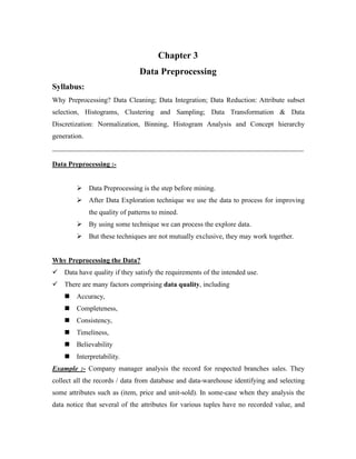
Histogram

16. Clustering
Clustering techniques consider data tuples as objects. They partition the objects into
groups, or clusters, so that objects within a cluster are “similar” to one another and
“dissimilar” to objects in other clusters.
Similarity is commonly defined in terms of how “close” the objects are in space,
based on a distance function. The “quality” of a cluster may be represented by its
diameter, the maximum distance between any two objects in the cluster.
Centroid distance is an alternative measure of cluster quality and is defined as the
average distance of each cluster object from the cluster centroid (denoting the “average
object,” or average point in space for the cluster). In data reduction, the cluster
representations of the data are used to replace the actual data.
Sampling
Sampling can be used as a data reduction technique because it allows a large data set
to be represented by a much smaller random data sample (or subset). Suppose that a large
data set, D, contains N tuples. Let’s look at the most common ways that we could sample
D for data reduction,
Simple random sample without replacement (SRSWOR) of size s:
This is created by drawing s of the N tuples from D (s < N), where the probability of
drawing any tuple in D is 1=N, that is, all tuples are equally likely to be sampled.
Simple random sample with replacement (SRSWR) of size s:
This is similar to SRSWOR, except that each time a tuple is drawn from D, it is
recorded and then replaced. That is, after a tuple is drawn, it is placed back in D so that it
may be drawn again.
Cluster sample:
If the tuples in D are grouped into M mutually disjoint “clusters,” then an SRS of s
clusters can be obtained, where s < M. For example, tuples in a database are usually
retrieved a page at a time, so that each page can be considered a cluster. A reduced data
representation can be obtained by applying, say, SRSWOR to the pages, resulting in a
cluster sample of the tuples.

17. Stratified sample:
If D is divided intomutually disjoint parts called strata, a stratified sample of D
is generated by obtaining an SRS at each stratum. This helps ensure a representative
sample, especially when the data are skewed.
For example, a stratified sample may be obtained from customer data, where a
stratum is created for each customer age group. In this way, the age group having the
smallest number of customers will be sure to be represented.
An advantage of sampling for data reduction is that the cost of obtaining a
sample is proportional to the size of the sample, s, as opposed to N, the data set size.
Hence, sampling complexity is potentially sublinear to the size of the data.

18.  Data Transformation and Data Discretization
In this Preprocessing step, the data are transformed or consolidated so that the
resulting mining process may be more efficient, and the patterns found may be easier
to understand.
Data Transformation Strategies Overview
In data transformation, the data are transformed or consolidated into forms
appropriate for mining. Strategies for data transformation include the following:
1. Smoothing, which works to remove noise from the data. Techniques include
binning, regression, and clustering.
2. Attribute construction (or feature construction), where new attributes are
constructed and added from the given set of attributes to help the mining process.
3. Aggregation, where summary or aggregation operations are applied to the data.
For example, the daily sales data may be aggregated so as to compute monthly and
annual total amounts. This step is typically used in constructing a data cube for data
analysis at multiple abstraction levels.
4. Normalization, where the attribute data are scaled so as to fall within a smaller
range, such as -1.0 to 1.0, or 0.0 to 1.0.
5. Discretization, where the raw values of a numeric attribute (e.g., age) are
replaced by interval labels (e.g., 0–10, 11–20, etc.) or conceptual labels (e.g., youth,
adult, senior). The labels, in turn, can be recursively organized into higher-level
concepts, resulting in a concept hierarchy for the numeric attribute. More than one
concept hierarchy can be defined for the same attribute to accommodate the needs of
various users.
6. Concept hierarchy generation for nominal data, where attributes such as street
can be generalized to higher-level concepts, like city or country. Many hierarchies for
nominal attributes are implicit within the database schema and can be automatically
defined at the schema definition level.
Discretization techniques can be categorized based on how the discretization is
performed, such as whether it uses class information or which direction it proceeds
(i.e., top-down vs. bottom-up). If the discretization process uses class information,
then we say it is supervised discretization.Otherwise, it is unsupervised.

19. Data discretization and concept hierarchy generation are also forms of data
reduction. The raw data are replaced by a smaller number of interval or concept
labels. This simplifies the original data and makes the mining more efficient.
Data Transformation by Normalization
 The measurement unit used can affect the data analysis.
 For example, changing measurement units from meters to inches for height, or from
kilograms to pounds for weight, may lead to very different results.
 In general, expressing an attribute in smaller units will lead to a larger range for that
attribute
 To help avoid dependence on the choice of measurement units, the data should be
normalized or standardized. This involves transforming the data to fall within a
smaller or common range such as [-1, 1] or [0.0, 1.0].
 There are many methods for data normalization. Such as;
 Min-max normalization
 z-score normalization
 z-score normalization mean absolute deviation
 Normalization by decimal scaling
 Min-max normalization
Min-max normalization performs a linear transformation on the original data.
Suppose that minA and maxA are the minimum and maximum values of an attribute, A
Min-max normalization maps a value, vi , of A to vi’in the range [new minA,new maxA]
by computing
vi’ = A
A
A
i
v
min
max
min


( new_maxA - new_minA) + new_minA
Example : Suppose that the minimum and maximum values for the attribute income are
$12,000 and $98,000, respectively. We would like to map income to the range [0.0, 1.0].
By min-max normalization, a value of $73,600 for income is transformed to
vi’ =
000
,
12
000
,
98
000
,
12
600
,
73


( 1.0 + 0.0) + 0 vi’ = 0.716

20.  z-score normalization
In z-score normalization (or zero-mean normalization), the values for an
attribute, A, are normalized based on the mean (i.e., average) and standard deviation
of A. A value, vi , of A is normalized to vi’by computing
vi’ = A
i A
v

'

A’ -- > mean
A
 -- > Standard Deviation
vi -- > Values
 z-score normalization mean absolute deviation
A variation of this z-score normalization replaces the standard deviation by the
mean absolute deviation of A. The mean absolute deviation of A, denoted sA, is
SA =  
|
'
|
|
'
3
|
|
'
2
|
|
'
1
|
1
A
vn
A
v
A
v
A
v
n













Thus, z-score normalization using the mean absolute deviation is
vi’ = A
i
S
A
v '

The mean absolute deviation, SA, is more robust to outliers than the standard deviation,σA
 Normalization by decimal scaling
Normalization by decimal scaling normalizes by moving the decimal point of
values of attribute A. The number of decimal points moved depends on the maximum
absolute value of A. A value, vi , of A is normalized to vi’ by computing
vi = j
i
v
10
where j is the smallest integer such that max (|vi|) < 1
j --> Digits from given data