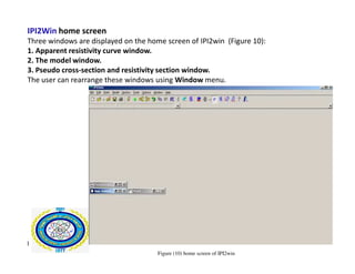
1. IPI2Win home screen
Three windows are displayed on the home screen of IPI2win (Figure 10):
1. Apparent resistivity curve window.
2. The model window.
3. Pseudo cross-section and resistivity section window.
The user can rearrange these windows using Window menu.
1
Figure (10) home screen of IPI2win
2. Interpretation of VES curves using IPI2win
IPI2win can be used for 1D interpretation of VES curves. Figure (11) shows the subsurface model used
in the 1-D sounding method. The layers are horizontal layers that have two parameters, the layer
resistivity ρ and thickness h (except for the last layer that is assumed to extend infinitely downwards).
VES curves could be analyzed with different arrays: Schlumberger, Wenner, and pole - pole. Figure
(12) shows interpretation VES curve using IPI2win.
Figure (11) A typical 1-D resistivity model.
2
Figure (12) 1-D model of vertical resistivity sounding data
3. The main steps for using IPI2Win
The main steps for using IP2Win are:
(1) Data input
(2) Data inversion
(3) Adding data points to create pseudo and resistivity sections.
Data input can be done directly from AB/2, V, I, and K data or AB/2 and ρ (Rho_a ) data.
The outputs are resistivity graph, resistivity-layer thickness table, and pseudo cross section.
Basic weakness of IP2 Win software is a bug that frequently occurs when analyzing data. That
problem can be solved by restarting software. The data collected from a 1-D resistivity
sounding survey consists of the electrode spacings used and the corresponding apparent
resistivity values.
resistivity values.
Data inversion : The purpose the inversion is to determine the thickness and resistivity of the layers
of a 1-D model that will produce a model response that matches the measured values. In this
method, an initial model is created, and the program modifies the thickness and resistivity
of the layers so as to reduce the difference between the calculated and measured apparent
resistivity values, see Figure (13).
Adding several data points can be used to create pseudo and resistivity sections.
Figure (13) Inversion of 1D VES data
3
4. VES data Input in IPI2Win
1. Run IPI2Win program and click File>New VES point or click New button on the toolbar. A new
VES window will come out, see Figure (14).
*AB/2 column is used for the distance between the current electrodes, MN column is used for the
distance between the voltage electrodes.
* SP is used for self potential data input, V for inputting voltage data, I for inputting electric current da
ta, and K is
the geometric factor data. Rho_a column is apparent resistivity data column (Rho_a is the result from
electrical resistance and geometric factor calculation value).
2. Choose the electrode array (Schlumberger for example) and apparent resistivity input.
3. Input the data (Ab/2 and Rho_a) as in the example (Figure 15). Points will be plotted in the graph.
Figure (14) New VES window
4
5. 4. Click OK to save the Data. (Note: Data can be saved in*.txt format by clicking Save TXT button).
5.Save as window will come out to decide where the data will be saved as VES data file. Give it
a name, as example “Test”. Click Save button. Curves and table will be displayed (Figure 16).
5
Figure (15) VES data input
6. Note:
The table gives the resistivity of each layer displayed in ρ column.
Layer thickness is displayed in h column. Layer depth from surface is displayed in d column.
Alt column is altitude column or depth from VES point elevation
(the example showed VES value elevation in 0 m so Alt value is -1.5 m, if VES elevation
value in 5 m then Alt value will be 3.5 m).
Data error is displayed on table title bar (error level in the example above is about 23.5%). Data error
can be corrected automatically by clicking Point>Inversion.
6 Figure (16) VES Curves
7. VES data inversion in IPI2 Win
1.Choose Point >Inversion command or click inversion button on the toolbar . The results will be
displayed and error value on table title bar will be changed, as shown in Figure (17) . (note:
there was a value decreasing from 23.5% to 6.82 %). Black curve shows the observed data. Red
curve shows the calculated curve and Blue curve gives information about resistivity variations.
2.Close IPI2 Win software by clicking File>Exit or Exit button on the toolbar.
Note: Every change made in IPI2 Win will be automatically saved.
Run IPI2 Win software again to input another VES point data.
Figure (17) Inversion results
7