2- AUTOMOTIVE LONGITUDINAL DYNAMICS (ACCEL, BRAKING, CRASH)

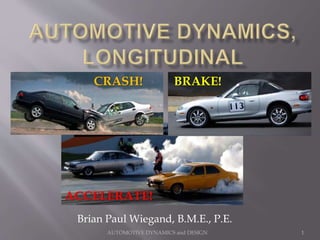
AUTOMOTIVE DYNAMICS and DESIGN 1
Brian Paul Wiegand, B.M.E., P.E.
CRASH!
ACCELERATE!
BRAKE!

2
AUTOMOTIVE DYNAMICS and DESIGN
LATERAL “WEIGHT
TRANSFER”
LONGITUDINAL
“WEIGHT TRANSFER”
WHEELSPIN

3
The difficulty of obtaining a
solution to the automotive
longitudinal acceleration
problem is belied by the
apparent simplicity of the
underlying relationship: "F
= m a". Consider the matter
of the accelerative force "F".
Values for the automotive
accelerative force must
ultimately be derived from
torque-speed relationship of
the particular engine
involved, such as that
depicted here:

4
The curve depicted is fairly
representative of internal combustion
reciprocating engines, with a low
torque output at low engine speed.
This is exactly the opposite of the ideal
for an automotive propulsion unit: high
torque at stall. To be made suitable for
automotive use, the torque-speed
relationship inherent in the piston
engine must be modified in
transmission to the drive wheels.
Depending on engine speed, the
appropriate torque values from the
WOT curve are translated and
transmitted through the drivetrain
resulting in accelerative forces at the
drive wheels, which becomes the net
accelerative force "F" when the rolling
resistance force "FR" and the aero-
drag force "D" are subtracted:
Where:
F = The accelerative force (lb, kg).
T = Engine torque (lb-ft, kg-m).
TR = Transmission torque ratio
(dimensionless).
TE = Transmission energy efficiency
(dimensionless).
AR = Axle torque ratio (dimensionless).
AE = Axle energy efficiency
(dimensionless).
RD = Dynamic rolling radius at drive
wheels (ft, m).
FR = Tire rolling resistance force (lb,
kg).
D = Aerodynamic resistance force (lb,
kg).

While the rolling resistance force
“FR”…
…and the aerodynamic drag force
“D”…
…are explicit and obvious functions of
vehicle velocity, the engine torque also
relates directly to velocity, at least after
the initial transient "start-up" of an
acceleration run. The relation between
engine speed and vehicle speed is:
5
Symbols unique to these equations:
rpm = Rotational speed of engine
(“revolutions” per minute).
V = Velocity of vehicle (mph, kph).
K = Translational to rotational
motion units constant
(14.005635 for “V” in mph and
“RD” in ft).
CR = Dynamic coefficient of tire
rolling resistance (lb/lb-
mph2.5).
KR = The static coefficient of tire
rolling resistance (lb/lb).
N = The “normal” (weight) load
on a tire (lb).

6
Following a somewhat circular chain of reasoning, it
can be shown that automotive acceleration is to
some extent a function of itself:
a = f(F)
F = f(T) >>>> a = f(T)
T = f(rpm) >>>> a = f(rpm)
rpm = f(V) >>>> a = f(V)
V = f(a, t) >>>> a = f(a, t)
This indicates that it will not be possible to put the
dependent and independent variables in
correspondent form; that the ultimate relation will be
transcendental. Transcendental equations can’t be
solved by algebraic means; transcendental relations
are amenable only to numeric approaches.

7
Moreover, the accelerative force generated by the engine is limited
in application by the available traction at the drive wheels. This
traction is dependent on the normal loads at the tires. These
normal loads are heavily influenced by the accelerative “weight
transfer” and “torque reaction”. In other words, there is yet more
reason to suspect a futility inherent in direct algebraic attempts at
solution.

8
Further analytic difficulty derives from the "m" variable of the basic relation
"F = m a". This "m" is not just a matter of vehicle weight divided by the
gravitational constant as would be the case with a simple homogeneous
body. An automobile is not a homogeneous body; some components are not
just accelerated translationally, but rotationally as well. To account for the
overall effects of this variegated behavior the concept of "effective mass" or
“me” must be substituted for the fundamental mass "m”:
The symbols unique to this equation are as follows:
W = The weight of the vehicle (lb, kg).
g = The gravitational constant, required only for English units (32.174 ft/s2).
I1 = Rotational inertia about front axle line (lb-ft2, kg-m2).
I2 = Rotational inertia about the crankshaft axis (lb-ft2, kg-m2).
I3 = Rotational inertia about transmission 3rd motion axis, plus 1st and 2nd
transmission motion axis inertias translated to the 3rd motion axis (lb-ft2,
kg-m2).
I4 = Rotational inertia about rear axle line (lb-ft2, kg-m2).

9
A concrete appreciation of how the individual terms in the effective
mass equation contribute to the total effective mass can be
obtained through study of an example set of parameter values
representative of an actual passenger car. For this purpose a 1958
Jaguar XK150S was taken to be representative of conventional
configuration passenger cars:

10
Considering just those basic aspects of the acceleration
problem as have been discussed so far, it should be apparent
that the automotive longitudinal acceleration relation is:
In view of the theoretical and practical complications
inherent in the automotive longitudinal acceleration problem, it
should not be surprising that an analytic solution is not
possible. Yet, despite the lack of an analytic solution, over
eighty years ago engineers were able to predict accelerative
performance with fair accuracy using a method of “hand”
calculation and graphical integration.
• Extremely complex, non-linear, encompassing many
variables.
• Consisting of numerous interconnected sub-
relations such that the total problem is perhaps best
expressed as a series of partial differential equations.
• Discontinuous by virtue of the gear changes and the
transient condition at the start of the acceleration run.

11
The traditional “hand” method of automotive acceleration performance
has been called the "Koffman Method", after the English engineer J. L.
Koffman who in the 1950's published a series of articles the
"Automobile Engineer". However, the essence of the method was a
part of common practice long before the appearance of Koffman's
articles. Certain authorities have credited the origin of the method to
the English professor W.E. Dalby, F.R.S., in the 1930's. Whatever the
origin of the method, what is important is that it circumvented the lack
of an analytic solution by utilizing desk calculators and drafting
equipment. Besides being tedious and slow, the limitations of such an
approach necessitated that certain aspects of the acceleration problem
be simplified:
•Neglect of “weight transfer” and its effects (vertical c.g. not
input).
•Neglect of “torque reaction” and its effects (track not input).
•Neglect of rolling radius variation (rolling radius held constant).
•Neglect of any initial or transient conditions (problems of initial
engine rpm, wheel spin, clutch slip, etc, were not addressed;
longitudinal c.g. was not input).

12
Traditional “hand” method utilized fact that the maximum
acceleration was obtained at WOT with “upward” gear shifts at
every intersection point of the acceleration-in-gear curves
(except if redline occurs first):

13
In contrast to "hand" calculation approaches to acceleration
performance problems, a computer simulation has the following
inherent advantages:
• Less time-intensive.
• Consistent results from analysis to analysis due to a
constant methodology and application.
• More significant digits, less round-off error.
• Constitutes a more readily transferable form of
knowledge (if properly documented) which results
in less demanding personnel requirements.
• Greater accuracy through smaller incrementation size.
• More realistic model possible with fewer
simplifications.
• Facilitates a systems engineering approach to design,
resulting in an optimized system as opposed to a
collection of optimized parts.

14
A simulation program termed "MAXGLONG.BAS“ was written in 1984.
The automotive acceleration problem may be divided into two distinct
stages, which is reflected in the simulation having two parts: the
“starting method” and the “continuing method”. The driving or
independent variable was taken to be the velocity, which relates directly
to engine rpm.
The starting method addresses the fact that at the commencement of
the acceleration run (t = 0, V = 0) not all the boundary values are known,
principally the initial engine rpm. This initial rpm (“rpm1”) is determined
on the basis of finding the maximum rpm on the WOT torque-rpm curve
for which the corresponding torque value does not cause wheelspin
(with its attendant decrease in traction). This is not as simple a problem
as it might seem, for the attainment of this maximum initial acceleration
is not instantaneous. Clutch slip, "wind-up" in the drivetrain, tire
deformation slip, etc., all ensure a transition period of some
milliseconds between “a = 0” and “a = maximum”; enough time for a
“weight transfer” to take effect modifying the acceleration potential. The
problem is therefore circular and requires some iteration for solution.
How this solution is obtained may be best understood by considering
the flowchart of the initial-engine-rpm subroutine…

15

16
After the clutch is engaged at the initial engine rpm, there
ensues the transient period of simultaneously decreasing engine
rpm and increasing vehicle velocity. What is happening during this
period is that the kinetic energy of the rotational mass "I2" is in the
process of being "shared" with the mass of the entire vehicle. The
engine rpm ceases to drop when an energy balance is achieved at
some lower rpm (“rpm2”):
The energy output by the engine “E” during this period of rpm
drop is generally not much of a factor, at least not for
conventional passenger vehicles. What is important is that
“rpm1” and the inertial quantity “I2” are large enough so that
“rpm2” is not equal to, or less than, the engine stall rpm. The
flowchart of the subroutine to determine “rpm2” is…

17

18
The determination of “rpm2” marks the transition between the
starting method and the continuing method. The continuing
method is actually the average of two different approaches to the
same end. The “interpolation” approach is predicated on an
assumed short-term linear relation between vehicle velocity and
the accelerative force, and is derived directly from the basic
relation "F = m a". For this approach the elapsed time and
traversed distance increments are determined by:

19
The “integration” approach is predicated on a curvilinear
relation between vehicle velocity and accelerative force. In this
connection the assumed parabolic torque-rpm model is utilized
to allow the necessary integration to derive the elapsed time and
traversed distance increment expressions:

20
The reason for the use of the average of these two sets of “Δt”
and “Δs” figures is graphically illustrated below; it is only the
averaged time and distance increments that allow the
MAXGLONG.BAS program to closely mimic the empirical velocity-
time curve:

21
This average value algorithm step is labeled “CALC TIME, DISTANCE
INCREMENTS & SUM” in the continuing method flowchart :

22
It should be noted that in the case of the MAXGLONG.BAS program a
very complex reality had to be reduced to a handful of simple
algorithms. A certain amount of arbitrariness was introduced in the
choice of “adjustment” factors to account for clutch slip, and in the
choice of a “three-point parabolic spline” as the torque-rpm curve
function. For instance, the parabolic torque-rpm curve is very well
suited to the actual torque-rpm nature of the Jaguar XKl50S engine,
but would not be so well suited to the Porsche 944 engine (the torque-
rpm curve is almost flat in the 2500-5500 rpm range). For a simulation
of a vehicle with such a flat torque-rpm relation, the “integration”
portion of the continuing method algorithm would have to be disabled,
and a “table look-up” with linear interpolation substituted for the
parabolic torque-rpm subroutine. This is not to denigrate the utility of
the program, it’s just that for each basic configuration to be analyzed
the procedure is not just a matter of “type in the parameters and run”.
Some adjustment or “bedding-in” of the program may first be
necessary by means of a known “benchmark” or “baseline” run.
Otherwise, the results may have a relative validity with respect to each
other but not necessarily much of a relation to reality.

23
THE MAXGLONG.BAS INPUT FILE:

24
THE MAXGLONG.BAS OUTPUT FILE (SHORT FORM):

25
FOR THE MAXGLONG.BAS VALIDATION THREE
VARIENTS OF THE 1958 JAGUAR XK150S WERE
USED:

26
FOR THE MAXGLONG.BAS VALIDATION THREE
VARIENTS OF THE 1958 JAGUAR XK150S WERE
USED:
ONE
TWO
THREE

27
•MAXGLONG.BAS NOTES:
AN INPUT FILE TEMPLATE, A COPY OF “MASS
PROPERTIES AND AUTOMOTIVE LONGITUDINAL
ACCELERATION” PAPER, AND PROGRAM FILE OF
MAXGLONG.BAS / SAMPLE INPUT & OUTPUT FILES /
LINE EDITOR / BASIC INTERPRETOR WILL BE
PROVIDED EVERY INTERESTED STUDENT.
•OTHER ACCELERATION PROGRAMS:
“STRAIGHTLINE ACCELERATION SIMULATOR” BY J.
TODD WASSON OF PERFORMANCE SIMULATIONS.
THERE ARE MANY OTHERS AVAILABLE WITH VARYING
DEGREES OF ACCURACY AND EASE OF USE.

28

29
Braking is just the reverse of acceleration; just as
effective mass was very significant with regard to
acceleration, it also is important with regard to braking.
The simplest (2-dimensional) depiction of a braking
vehicle of weight “Wt” initially moving with a velocity
“V”, but sliding to a stop in a distance “d”, is:

30
The only force in line with the vehicle displacement is the
dynamic friction force “f”, so this is the only force doing any
work. The total work done by “f” between Point 1 and Point 2
is “f × d”, and since “f” is directionally opposite the
displacement this represents negative work. If the vehicle
comes to a complete stop (“V = 0”) at Point 2, then the friction
work done at that point has completely dissipated (equaled)
the vehicle’s kinetic energy as it existed at Point 1, where the
braking effort was initialized:

31
However, braking to a stop requires dissipating
all the kinetic energy of the vehicle, which
means not just the energy associated with the
translationally moving mass, but all the
rotationally moving mass as well. Substituting
for “m” the “me” of previous discussion, but
dropping the “I2” term for a “clutch disengaged”
condition, brings the model a little closer to
reality:

32
Another step toward reality involves “f”; there is no such
single force acting on the vehicle to slow it down. There
are traction forces (“ff”, “fr”) at the tire/ground contact
points, which result from forces at the brake friction
surfaces generating rotation resisting torques (“Tf”,
“Tr”), and then there are rolling resistance forces (“FRf”,
“FRr”), plus an aerodynamic drag force (“D”):

33
Even this model is not completely realistic. However, it does
show the aero forces “D” (drag) and “L” (lift) acting at the
“CP” (center of pressure). More importantly, it now shows the
individual traction forces at the front and rear (2-dimensional
model) tire/road contact areas, and indicates how those
forces are influenced by longitudinal “weight transfer” (which
is modified due to the aero moments) resulting from the “ma
× h” moment:

34
The previous equation revised in accord with this
greater realism is:
The aero drag “D” and lift “L” forces may be calculated
(with “V” now in feet-per-second) per:
The areas “Af” and “Ap” are in square-feet and the
resulting “D” and “L” forces are in pounds.

35
The rolling resistance at the front axle “FRf” and the
rolling resistance at the rear axle “FRr” are expressed
by the equations:
FRf = CSf Nf + 3.24 CDf (V/100)2.5 Nf FRr = CSr Nr + 3.24 CDr (V/100)2.5 Nr
Here the velocity “V” is in units of mph, while the axle
normal forces “Nf” and “Nr” and the resulting axle
rolling resistance forces ““FRf” and “FRr” are all in
terms of pounds. The axle traction forces associated
with braking “ff” and “fr” are also dependent on the
axle normal loads “Nf” and “Nr” :
However, complication results from the fact the
traction coefficients “μf” and “μr” are themselves a
function of normal load…

36
…or, more precisely, functions of contact area
pressure “Pc” (since “Pc = N/Ac”):
Some typical tire specific values for “a” and “n” might
be “15.7369” and “-0.67791”, respectively. The
“15.7369” is the value of “a” for pressure units in psi;
for pressure units in kPa use “58.2587” for “a”. Of
course, the contact areas will also vary in accord with
the normal loads…

37
The front and rear tire contact areas (multiply by ”2”
for axle area) vary in accord with normal loads per:
Where:
Ac = Tire to ground plane gross
contact area (in2)
Lc = Tire to ground contact area
length (in).
tw = Tire tread width, assumed
constant with load (in).
Ri= Tire no-load inflated radius
(in).
d = Tire vertical deflection under
load (in).

Where for these last two equations:
KZ = Tire vertical stiffness (lb/in).
tw = Tire tread width, assumed constant with load (in).
= Tire section aspect ratio (dimensionless).
SN = Tire nominal section width (mm).
N = The normal load on the tire (lb).
d0 = Tire deflection function “y-intercept” value (in).
38
To use those area equations requires calculation of the tire
deflection “d” under normal load “N” (lb)…
…and also requires the width of the tire tread “tw” which, when
lacking a measured value, can be approximated per the
formula:

39
Note the deflection equation further requires
calculation of the tire vertical spring rate “Kz”:
Where:
KZ = Tire vertical stiffness (kg/mm).
Pi = Tire inflation pressure (kPa).
= Tire section aspect ratio (dimensionless).
SN = Tire nominal section width (mm).
DR = Wheel rim nominal diameter (mm).

40
An initial concentration on the normal loads would seem
to be key; the normal loads, which result from the static
longitudinal weight distribution as modified by dynamic
“weight transfer” and by aerodynamic drag and lift are:
Where:
Wt = Total vehicle weight (lb).
Wb = Vehicle wheelbase (in).
LCG = Longitudinal distance of CG from front axle (in).
me = Vehicle “effective mass” (lb).
a = Vehicle deceleration (in/sec2).
VCG = Vertical distance of CG from ground plane (in).
D = Aerodynamic drag force (lb).
VCP = Vertical distance of CP from ground plane (in).
L = Aerodynamic lift force (lb).
LCP = Longitudinal distance of CP from front axle (in).

41
The brakes on any modern car can easily “lock” the wheels, but
that is not maximum longitudinal deceleration. For maximum
longitudinal deceleration the braking force “f” must be exactly
equal, not greater than the maximum static traction force “N μ”
that the tires are capable of. This means that the torque “T”
produced by the brakes can not be more than “f R”:
Traditionally this means that a lot of time and effort was spent on
developing brake proportioning systems, and later Anti-skid
Braking Systems (ABS). Skilled drivers and modern ABS can be
so good that the above equations of perfect brake balance may be
assumed to hold. It is this assumption of perfect brake
proportioning which makes the functioning of the braking
computer simulation program “MAXDLONG.BAS” possible.

42
THE MAXDLONG.BAS FLOW CHART:

43
THE MAXDLONG.BAS INPUT FILE:

44
THE MAXDLONG.BAS OUTPUT FILE (SHORT FORM):

45
THE MAXDLONG.BAS VALIDATION:

46
* AN INPUT FILE TEMPLATE, AN EXCERPT FROM “MASS
PROPERTIES AND ADVANCED AUTOMOTIVE DESIGN”, AND
PROGRAM FILE OF MAXDLONG.BAS / SAMPLE INPUT & OUTPUT
FILES WILL BE PROVIDED EVERY INTERESTED STUDENT WHO
HAS SURVIVED SO FAR.
* OTHER BRAKING SIMULATION PROGRAMS:
ADAMS (Automatic Dynamic Analysis of Mechanical Systems)
computer programs as used to model and simulate the performance of
an anti-lock braking system (as written about by B. Ozdalyan and M.V.
Blundell, Sch. of Eng., Coventry Univ., UK) .
CarSim is a commercial software package that predicts the
performance of vehicles in response to driver controls (steering, throttle,
brakes, clutch, and shifting) in a given environment (road geometry,
coefficients of friction, wind). CarSim is produced and distributed by an
American company, Mechanical Simulation Corporation, using
technology that originated at The U. of Michigan Transportation
Research Institute (UMTRI).

47

48
Automotive safety has two main aspects: the “active”
and the “passive”. The “active” aspect of automotive
safety is the subject of accident avoidance, which
involves such things as acceleration, braking,
cornering, maneuverability, and directional stability;
each of which is a complex subject in its own right.
Also there are safety aspects not inherently part of
automotive design; such as roadway construction,
speed limits, and traffic regulation. What is the sole
concern of this crash segment is the “passive” aspect
of automotive design: the minimization of automotive
crash consequences: fatality, injury, and property loss.
Of those three consequences fatality is the most grave,
making crash survival the greatest imperative of
automotive design!!!

49
Crash survival is a matter of reducing the magnitude of
injury and thus the likelihood of death. To reduce the
magnitude of injury one must begin by considering the
human physique which, like any other structure,
is prone to failure when subjected to excessive stress
levels; stress “S” is expressed as force “F” per area
“A”:
S = F/A
The forces associated with the deceleration of
the masses act in accord with Newton’s Second Law
of Motion:
F = m a

50
By combining those two equations it becomes
obvious that injurious or fatal stresses inflicted upon
the human physique by sudden decelerations may be
reduced in two ways:
S = m a / A
One way is to increase the areas (“A”) over which the
forces are distributed, and the other way is to decrease
the decelerations (“a”) involved. Hence the modern
emphasis on padded dashboards and recessed hard
points for automotive interiors, and the ancient
emphasis upon helmets and armor in combat; it was all
an attempt to dilute the forces involved.

51
The survivable limits of human deceleration are
not clear-cut. A great deal depends on the particular
individual involved and on the particular
circumstances of the accident. A burly longshoreman
is physically quite different from a petite secretary, but
which one would be the most likely to survive
dangerous impact loadings? This depends on
physiological factors which are not necessarily visible
or even readily identifiable; microscopic matters such
as cell structure and capillary formation may be
involved. Macroscopically, a sturdy skeleton and
robust configuration must be weighed against the
disadvantage of greater mass. Genetics, sex, age, size,
nutrition, physical condition and many other factors
may play a part in determining individual deceleration
limits.

52
What is known is that there are six general
survival criteria factors which are amenable to
manipulation; these factors are:
1. Magnitude of the Deceleration
(usually measured in gravity
units or “g’s”).
2. Rate of Onset of the Deceleration
(also known as “jerk”, which is
the rate of variation in the
deceleration level, usually
measured in “g’s/sec”).
3. Duration of the Deceleration (the
time elapsed at some
deceleration level, usually
measured in “seconds”).
4. Position/Packaging (orientation of
the subject with respect to the
deceleration vector, and then
maintaining that orientation.
5. Vibration (impact vibration is a
highly intense random
oscillation over a very short
time span, so a statistical
approach is required that
quantifies the power of each
vibration input over the
frequency range).
6. Angular Acceleration (measured
in degrees or radians per
second squared; angular
acceleration rates at onset, at
peak, and throughout the
duration are all significant).

53
(Koelle, H.H. (Editor-in-Chief); Handbook of Astronautical Engineering, NY, NY;
McGraw-Hill, 1961, pg. 26-42)

54
The “Lovelace Chart” presents the approximate
deceleration level limits for human survival.
However, severe deceleration events leading to
near human fatality generally do not have
accelerometers present, so for events like near
fatal automobile accidents the “g” levels can only
be estimated from such data as can be recorded at
the scene. The survived incident of the “55 ft
(16.76 m) fall with 4 in (10.16 cm) deceleration”
provides enough such information that the
estimation technique used to produce the chart
may be determined.

55
Since the deceleration distance is 4 in or 0.33333
ft, the following distance-average deceleration “ā”
equation can be written:
Into this equation the known values may be
“plugged”:

56
There are two unknowns, the average
deceleration “ā” and the duration time “t”, so one
more equation is necessary for solution. The
velocity change with time provides this:
Again, the known values may be inserted:

57
“Solving” this for “t” results in:
Substituting this for “t” in the distance equation
results in:

58
This may now be solved for the average deceleration
“ā” resulting in:
Since 141.0 g’s is close (97%) to the chart-indicated
deceleration rate of 145 g’s, it is reasonable to
assume that average deceleration calculations such
as this just carried out were used to estimate the
deceleration levels for the “severe auto accidents”.
This is notable as it means that deceleration levels
significantly greater than the indicated average
deceleration levels of the chart were endured and
survived (though for shorter duration!).

59
“David Charles Purley…(26 January 1945 – 2 July
1985) was a British racing driver… best known for
his actions at the 1973 Dutch Grand Prix, where he
abandoned…(his race car)…and attempted to
save…fellow driver Roger Williamson, whose car
was…on fire...Purley was awarded the George
Medal for his courage in trying to save Williamson,
who suffocated...During pre-qualifying for the 1977
British Grand Prix Purley sustained multiple bone
fractures (when)…he crashed into a wall. His
deceleration from 173 kph (108 mph) to 0 in a
distance of 66 cm (26 in) is thought to be one of the
highest G-loads in human history…He died in a
plane crash in…1985.”

60
“…(Purley) survived an estimated 179.8 g’s when
he decelerated from 173 km/h (108 mph) to 0 in a
distance of 66 cm (26 inches)… This was the
highest measured (sic) g-force ever survived by a
human being…(until in 2003, Kenny Bräck’s crash
violence recording system measured 214 g’s)…”
Using the same methodology as previous we may
make our own estimate of the average Purley G-
load:

61
(Koelle, H.H. (Editor-in-Chief); Handbook of Astronautical Engineering, NY,
NY; McGraw-Hill, 1961, pg. 26-43)

62
(Harris, Cyril, and Charles E. Crede; Shock and Vibration Handbook, NY,
NY; McGraw-Hill, 1961, pg. 44-43)

63
(Koelle, H.H. (Editor-in-Chief); Handbook of Astronautical Engineering,
NY, NY; McGraw-Hill, 1961, pg. 26-36.)

64
“The study of the automobile …shows that complete body support
and restraint of the extremities provide maximum protection
against accelerating forces and give the best chance for survival. If
the subject is restrained in the seat, he makes full use of the force
moderation provided by the collapse of the vehicle structure, and is
protected against…bringing him in contact with interior
surfaces…”
( Harris, Cyril, and Charles E.
Crede; Shock and Vibration
Handbook, NY, NY; McGraw-
Hill, 1961, pg. 44-34.)
(A concept of the course
instructor’s regarding “good “
packaging of the automotive
occupants )

65
Harsh fluctuating deceleration input compounds any detrimental
effects on the human physique, and even more so if it should
excite “resonance” of any of the internal organs (for example, the
natural frequency of the Thorax-abdomen system of a human
subject is between 3 and 4 cps…). In such a case large organ
displacement effects are possible, even when the exciting
deceleration inputs may be relatively small. The aerospace
technique used to combat the effects of such vibration, which has
similarity to the vibration characteristic of aerodynamic buffeting,
rocket liftoff, re-entry splashdown, etc., is to prevent internal
organ displacement by use of a tight fitting garment of flexible but
inelastic material: a “g-suit”. Obviously the expedient of dressing
up like an astronaut just to drive to the local market is impractical
for everyday automotive application (and we won’t even talk
about the “immersion” technique lest someone design a
combination car and swimming pool!).

66
Angular acceleration warrants being listed as a
major factor in crash survival due to the human
brain’s particular sensitivity to sudden rotational
movements. Boxers have long been aware that a
cross or a hook can be more effective than a jab of
equal magnitude; any blow that tends to twist the
head about the neck is generally rated high in
effectiveness. This is especially interesting in light
of the fact that about 70% of all automotive
fatalities are caused by head/neck injuries. Many of
these fatal injuries involve tearing of the tissue at
the back of the brain stem area, and much of that
is due to rotational shearing effects.

67
THE CHARACTER OF AUTOMOTIVE CRASHES MUST BE
STUDIED IN HOW IT RELATES TO THE SURVIVAL
FACTORS…
Edeform = Etranslation + Erotation + Eengine - Elosses
THE AREA UNDER THE “CURVE” REPRESENTS THE
ENERGY USED IN CRUSHING THE VEHICLE
STRUCTURE, WHICH IN TURN IS RELATED TO…

68
THE “Etranslation + Erotation “ REPRESENTS THE TOTAL
KINETIC ENERGY POSSESSED BY THE VEHICLE AT THE
TIME OF IMPACT, WHICH BRINGS US BACK TO OUR OLD
FRIEND “EFFECTIVE MASS”:
Edeform = Etranslation - Elosses
THE REASON WHY THAT IS NOT MORE EMPHASIZED IS
BECAUSE IN A CRASH IT IS NOT POSSIBLE TO BE VERY
CERTAIN HOW MUCH OF THE KINETIC ENERGY WILL
BE UTILIZED FOR DEFORMATION. SOMETIMES THE
ROTATIONAL ENERGY ISN’T EVEN CONSIDERED:

69
ENERGY PRODUCED DURING A FRONTAL CRASH BY
THE ENGINE “Eengine” IS MINISCULE, AND THE
ROTATIONAL KINETIC ENERGY OF THE ENGINE AND
MUCH OF THE DRIVETRAIN TENDS TO GET “LOST”:

70
ENERGY IS ALSO “LOST” TO THE DEFORMATION OF
PRIMARY STRUCTURE DUE TO THE SHEDDING OF MASS
DURING A COLLISION:

71
Energy can also be dissipated in a number of
other ways: light, sound, vibration, heat, and
friction. An automotive crash usually involves all
of these forms of energy dissipation, but primarily
it is by work, the deformation of the vehicle
structure, that most of the available vehicle
kinetic energy is dissipated. However, exactly
how much energy that is constitutes a problem.
As a rough “rule of thumb”, for full frontal
collisions take the effective weight to be the crash
weight plus an extra 3.7 percent to account for
any rotational energy input.

72
1954 TWO CAR HEAD ON CRASH TEST:
(Harris, Cyril, and Charles E. Crede; Shock and Vibration Handbook, NY,
NY; McGraw-Hill, 1961,pg. 44-48)

73
1963 HEAD ON BARRIER CRASH TEST:
(Patrick, Laurence M. (Editor); 8th Stapp Car Crash and Field Demonstration
Conference, Detroit, MI; Wayne State University Press, 1966, pg. 296-297)

74
THE FACT THAT THE DECELERATION TRACE CAN VARY ALL
OVER THE HUMAN BODY AND BE SIGNIFICANTLY AT VARIANCE
WITH THE MAIN VEHICLE TRACE USUALLY BODES ILL FOR THE
VEHICLE OCCUPANTS, BUT CAREFUL ENGINEERING CAN MAKE
BENEFICIAL USE OF SUCH A SEPERATION OF OCCUPANT
DECELERATION BEHAVIOR FROM THAT OF THE CAR:

75
“The available space for seat or passenger travel using the principle of
energy absorption…must be considered carefully…seat belts and other
crash restraint(s)… (using) extensible fabrics have been found to be
extremely hazardous since their load characteristics cannot be
sufficiently controlled…increase in exposure time must be considered as
well as the reduction in peak acceleration. For very short exposure times
where the body’s tolerance…is…not (limited by) the peak acceleration,
the benefits derived from reducing the peak loads would disappear.”
“Many attempts have been made to incorporate energy-absorptive
devices…in a harness or in a seat with the intent to change the
acceleration-time pattern by limiting peak accelerations…The benefits
derived from such devices are usually small since little space for body or
seat motion is available in…automobiles…”
(Harris, Cyril, and Charles E. Crede; Shock and Vibration Handbook, NY, NY;
McGraw-Hill, 1961, pg. 44-35 and pp. 44-34 to 44-35.)
.

76
1976 HEAD ON BARRIER CRASH TEST:
(Ishisaka, Takashi; Masanori Tani, Osamu Fujii, and Kyosuke Hamada; “Analysis of
Crashworthiness of Automobile Body in Collision (Simulation of Frontal Collision)”,
Mitsubishi Heavy Industries Technical Review, June 1976, pg. 130).

77
For impact velocities of around 30-35 mph (48-56 kph), the automotive
barrier crash traces have been undergoing radical change for about
forty years. This effect started with FMVSS compliance testing, and
has accelerated with NCAP rating testing. NCAP frontal crash testing
for rating is very similar to the FMVSS 208 frontal crash testing for
compliance. Both involve full frontal crash into an immovable barrier,
but the NCAP requires impact at “35 mph” (56.3 kph) while FMVSS 208
requires impact at only “30 mph” (48.3 kph), which represents a 36%
difference in kinetic energy dissipation. Instrumented dummies are
used for both FMVSS and NCAP. Various acceleration, deflection, and
strain readings are taken from the instrumented dummies during the
crash duration from which four criteria are derived to rate the vehicle’s
frontal crash performance. Compliance tests require that only
“passive” restraints be used, which usually means seatbelts are
unfastened (unless they fasten automatically) and the dummies
generally have to rely on only the airbags for their salvation. NCAP,
however, allows the dummies the advantage of both belts and bags.

1) Head Injury Criterion (HIC), which for FMVSS compliance “traditionally” had to
be < 1000 for the 50th percentile “adult male” dummies serving as “driver” and
“passenger”, but “recent” changes involve a HIC limit of 700 and use of 5th
percentile “small adult female” dummy as “passenger”. As of MY 2011 NCAP
testing requires the 50th percentile “male” dummy as “driver” and the 5th percentile
“female” dummy as “passenger”.
2) Neck Injury Criterion is a relatively new requirement for FMVSS compliance;
for the 50th percentile dummy limiting neck tension/compression loads are 937/899
lb (4170/4000 N), and for the 5th percentile dummy are 589/566 lb (2620/2520 N).
Interestingly, NCAP neck injury measurements of 12 vehicles MY2011-MY2014
registered a max tension reading of 360 lb (1600 N).
3) Chest Acceleration/Compression Criterion, which for FMVSS compliance
“traditionally” had to be < 60 g’s (except where duration at this peak is < 3 ms) or <
3 in (7.62 cm) (this became 2.5 in or 63 mm after year 2000). Again, for NCAP
there are no pass/fail levels, but scoring under the compliance pass/fail levels
would seem to be commendable.
4) Femur Axial Load Criterion, which for FMVSS compliance “traditionally” must
be < 2250 lb (10 kN) for a 50th percentile “adult male”. NCAP only “recently”
included a < 1530 lb (6.8 kN) 5th percentile “small adult female” in its front crash
rating evaluation. 78

79
THE PRESENT HEAD INJURY CRITERIA FORMULATION:
Where:
HIC = Head Injury Criterion (dimensionless).
t1 = Time at start of interval of interest (seconds).
t2 = Time at end of interval of interest (seconds).
a = Resultant (total) deceleration (g’s) as per:

80
HEAD INJURY CRITERIA USAGE CIRCA 1980:

81
1999, THE EFFECT OF FMVSS AND NCAP:
“Over the past fourteen years of NCAP testing, on average, the total
crush…has increased, the peak deceleration…has decreased, and the time
duration…has increased. The trend…is consistent with a reduction in the
total stiffness of frontal structures…the less stiff have higher NCAP rating.”
(Park, Brian T., James R. Hackney, Richard M. Morgan, and Hansun Chan; “The New Car
Assessment Program: Has It Led to Stiffer Light Trucks and Vans Over the Years?”, SAE
International Congress & Exposition, Detroit, MI, March 1999, pp. 7-8, 14)

82
THE EFFECT OF FMVSS AND NCAP HAS BEEN TO MAKE
POSSIBLE THE CALCULATION OF THE FRONTAL CRASH
PERFORMANCE OF VEHICLES SOLD IN THE U.S., AS WILL
BE DEMONSTRATED.
(Note that problems in dynamics generally are solved
by use of any one or more of three basic methods:
force and acceleration, work and kinetic energy, and
impulse and momentum; these are just different ways
of looking at a common underlying reality. The
method(s) used to investigate a particular dynamics
problem depends upon the specific nature of the
problem. Problems involving that most severe form of
automotive longitudinal deceleration, crashing, often
requires the application of all three methods.)

83
WE START WITH SOME OF THE BASIC FORCE-
DEFLECTION FUNCTIONS:
SPRING (no
permanent
deformation
, increased
duration)
CONSTANT
(most stroke
efficient, high
rate of onset)
RAMP or
“PROGRESSIVE”
(intermediate
between Spring
and Constant)

84
MODERN SECONDARY AND PRIMARY STRUCTURE
FORCE-DEFLECTION FUNCTIONS:
INDEPENDENT BUMPER BODY DESIGN INTEGRATED BUMPER BODY DESIGN
GOOD DAMAGE PROTECTION,
HIGH RATE OF ONSET, NOT A
SMOOTH DECELERATION TRACE.
POOR DAMAGE PROTECTION,
LOW RATE OF ONSET, A SMOOTH
DECELERATION TRACE.

85
MODERN SECONDARY AND PRIMARY STRUCTURE
FORCE-DEFLECTION FUNCTIONS:
“…automobile companies are increasingly requiring that
bumpers contribute to the deceleration of the automobile in
high-speed crashes…”
(Krishnaswamy, Prakash; and Ayyakannu Mani, “Crash Codes Pave the
Way to Safer Vehicles”, Mechanical Engineering, April 1991, pg.61)
“…bumper system…designed to collapse at a predetermined
load level, which limits the load…transmitted to the…frame
structure.”
(Ibid, referring to a historical bumper illustration)
“The bumper and the support structure…(are designed)…so
that the bumper makes the necessary contribution to the
overall deceleration pulse.”
(Ibid, pg. 62)

86
THANKS TO NCAP WE CAN ASSUME THAT THE ENTIRE FRONTAL
CRUSH DISTANCE IS USED TO ABSORB ALL THE VEHICLE KINETIC
ENERGY IN A 35 MPH BARRIER CRASH:

87
The 1996 Dodge Neon and the 2006 Honda Ridgeline
will serve as representatives of the generic “small
light” and “large heavy” vehicles. To determine the
kinetic energy of each at 35 mph we will assume the
following about their “effective mass”:

88
The value for “F0” will be assumed sufficient to
generate an instantaneous deceleration value of 3 g’s
(probably overly generous), and the maximum force
“Ft” will be such that:
= 73,279 lb,
or 24.34 g’s
= 110,686 lb,
or 21.61 g’s
Which also tells us the max g’s of each vehicle in the
NCAP barrier crash:

89
The values for “F0” and “Ft”, along with the crush
distances “Xt”, allow us to draw the vehicle force-
deformation “curves” (note we have assumed zero
“spring-back”):

90
All of the assumptions and calculations made so far
allow us to determine what would happen if these two
generic representatives were to crash head on:

91
The “small light” car utilizes all its available crush
energy capacity, just as it did in the barrier crash:
= 123,303 ft-lb
While all the “small light” car’s crush distance (2.996
ft, 913.2 mm) is used, a considerably smaller crush
distance “x” is inflicted on the “large heavy” car. This
distance “x” is easily determined by using the
stiffness “KF” for the “large heavy” and the ultimate
force “F” generated between the two vehicles in the
equation:

92
Now the work energy expended on deforming the
“large heavy” car can be determined:
So the “large heavy” vehicle fares better than the
“small light” vehicle with less deformation at 2.022 ft
(616.3 mm) vs. 2.996 ft (913.2 mm), and less
deformation energy absorbed at 89,620 ft-lb (121.5 kJ)
vs. 123,303 ft-lb (167.2 kJ). Also, the “large heavy”
maximum deceleration is only 14.31 g’s while the “small
light” maximum deceleration is 24.34 g’s (same as in
the barrier crash). This indicates that a head-on crash
would be rough on the occupants of the “small light”
vehicle, but very easy on those in the “large heavy”
vehicle, which is in accord with reality.

93
This sort of result has been corroborated by actual
empirical observations:
“…the crush distances of the heavy
and light cars in rigid barrier impact
are…850 mm and 550 mm. Yet in a
head-on collision, by virtue of equal
forces at the interface, the heavier car
crush decreases to 620 mm while the
lighter car crush increases to 870
mm.”
(Prasad, Priya (Ed.); and Jamel E. Belwafa (Ed.), Vehicle Crashworthiness and
Occupant Protection; Southfield, MI; American Iron and Steel Institute, 2004, pg.
92)

94
Anyway, the performance of the “large heavy”
and “small light” vehicles together in the
“head-on” crash was quite different from the
individual barrier crash tests. This illustrates
why the NHTSA says that the (up to) “5-star”
(front crash) safety ratings can only be used to
compare vehicles within the same (weight)
class. Of course, these are only the results
with a head-on crash that did not violate the
“small light” vehicle’s passenger space;
anything more severe (but totally possible)
would have been very bad indeed for the
“small light” vehicle’s occupants)…

The difference is because a head-on crash between
two cars is fundamentally different from individual
barrier crashes! At the end of the barrier crash event
the velocity “V2” is zero (ignoring any velocity reversal
due to “spring-back”); the delta velocity is essentially
just “-V0” (DV = V2 -V1 = 0 – V0 = -V0). But in a head-on
crash between two cars the post-event velocity may
not be zero; the two cars may continue moving as a
unit at some reduced post-crash velocity. This means
that not all of the pre-crash kinetic energy (proportional
to the closing velocity “Vc” squared) gets utilized for
deformation of structure, just the energy associated
with twice the average delta velocity “ ” squared. For
such situations equations derived using the
methodology of impulse and momentum must be
employed. 95

96
The average delta velocity of this two vehicle crash
can be determined from the delta kinetic energy
involved and the work energy spent in deformation:
“
From this average it is easy to find the individual
vehicle “DV’s” if the momentum relation “DV2/DV1
= me1/me2” holds true, which means:
So, input the parameter
values:
and

97
So “plug in” the vehicle parameter values:
The average delta velocity would indeed seem to have
been about 28.0 mph. Of far more interest is what
would the closing velocity “Vc” have been, as that is
an important indicator of what constitutes an upper
limit on the severity of a crash before fatality occurs.

98
The closing velocity “Vc” is determined per the
formula:
Occupant Protection; Southfield, MI; American Iron and Steel Institute, 2004, pg.
91)
“Plugging in” the appropriate “small light” and
“large heavy” vehicle values results in:

99
So for the two vehicles considered here a closing
velocity of 57.9 mph constitutes the limit for a head
on crash without fatality. Note that the closing
velocity less the two individual delta velocities
leaves almost 2 mph (3.2 kph); the two wrecks
continued moving in unison post-crash at this
speed:
Vc - DV1 - DV2 = 57.9 – 35.21 – 20.70 = 1.99

100
Obviously this calculated maximum closing
velocity without fatality merely provides a
“figure of merit” by which the crash safety of
automotive designs may be judged; there is no
guarantee that a head on crash between the two
vehicles in question would not result in a fatality.
The closing velocity calculation provides us with
a “tool” to evaluate certain crash situations, to one
of which we already have an answer as it was
provided by the NHTSA itself. Let us see if our
“tool” provides us with the same answer…

101
NHTSA says that two cars of the same class
(explicitly a matter of weight but implicitly a
matter of size as well) performing well in the
NCAP 35 mph (56 kph) barrier crash will also
perform equally well together in a 70 mph (113
kph) head-on crash. We can use the already
calculated information on the “small light” (or
the “large heavy”) vehicle and conduct a thought
experiment wherein two identical vehicles
(thereby definitely of the same “class”)
experience a head on crash. Utilizing the “small
light” (1996 Dodge Neon) results in the
following…

102
The individual delta V’s in such a crash would be
identical:
The maximum closing velocity without fatality
(NHTSA : “performing well”) would be:
It would seem the NHTSA statement is verified, and
that our automotive crash analysis methodology is
fairly sound.

103
This methodology provides us with a rational way
to answer a number of questions involving
automotive crash (head on) safety:
•Can a “large heavy” weight vehicle and a “small light” weight
vehicle do equally well in the barrier crash test?
•If so, then how will the same vehicles fare in a head-on crash
against each other? That is, does the “large heavy” vehicle
necessarily fare better than the “small light” vehicle?
•Heavy vehicles tend to also be larger than light vehicles, but
what role does size play independent of weight? That is, if the
weight is equal, does the larger vehicle necessarily fare better?
•If, as commonly suspected, a “small light” car is at an inherent
safety disadvantage to a “large heavy” car, then what can be
done to “level the playing field”?

104
The answers may be divined from the following
summary of a number of calculated crash
possibilities:

105
From the investigations conducted, it would seem that the “small
light” car will always be at a great disadvantage in a crash to a
“large heavy” car given the way the current “safety system” works.
Designing a vehicle so as to minimize deceleration levels in a 35
mph (56.3 kph) barrier crash test only gives some assurance of
safety in a crash wherein a vehicle moving at 35 mph (56.3 kph)
impacts flush with, and orthogonal to, an immobile and unyielding
barrier. In real world crashes circumstances that exactly replicate
such conditions are rare; the structural softness required of small
light cars to score well in the NCAP barrier crash test ensures that
in many real world crashes the vehicle passenger space is
crushed and mangled. Since human tolerance to acceleration is
very high if properly “packaged”, it makes sense to stiffen the
structure of small light vehicles and to correspondingly enhance
the occupant “packaging”. Even if the stiffer structure were to incur
higher deceleration levels in an accident, the possibility of
surviving such levels beats the impossibility of surviving being
crushed or torn to pieces.

106
“When cars of the same wheelbase but different
mass collided, the driver of the lighter car was
more likely to be killed than the driver of the
heavier car. When cars of similar mass but different
wheelbase collided…the differences…were too
small to be detected by the same method…they
concluded that mass is the dominant causative
factor in the large dependence of driver fatality risk
on “size” in two-car crashes...”
(Fildes, B.N.; S.J. Lee, and J.C. Lane; “Vehicle Mass, Size, and Safety”, Report
No. CR133, Federal Office of Road Safety; Canberra, Australia, 1993., pg. 8)

107
The desire to score well in the 35 mph (56.3 kph) NCAP test
seemingly drives current automotive design. This situation has
certain consequences, not all of them beneficial:
“To absorb all the kinetic energy, which is
proportional to the square of the velocity, the
deformable structure length must have a specific
stiffness.”
“…designing vehicles for the NCAP testing promotes
the stiffness of the structure to be proportional to
the mass of the vehicle. The heavier the vehicle the
stiffer its front structure will be.”
(Witteman, Willem; “Adaptive Frontal Structure Design to Achieve Optimal
Deceleration Pulses”, Paper #05-0243, Proceedings of the 19th International
Conference on Enhanced Safety of Vehicles; Washington D.C., USA, 2005, pg. 1)
Occupant Protection; Southfield, MI; American Iron and Steel Institute, 2004, pg.86)

108
“The use of the same fixed deformable barrier in crash
tests for light and heavy cars could lead to less
compatibility in crashes between small and large
cars.”
“For compatibility it is necessary to have a stiffer
structure in case of a heavy opponent and a softer
structure in case of a lighter opponent.”

109
“…the majority of collisions occur with partial
frontal overlap and under off-axis load directions
against other cars with much greater or smaller
masses and structural stiffnesses. Realistic crash
tests with partial overlap have shown that
conventional longitudinal structures are not capable
of absorbing all the energy in the car front without
deforming the passenger compartment…To protect
the occupants the passenger compartment should not
be deformed and intrusion must be avoided…”

110
“…LTVs are a growing component of…US…vehicles
…incompatibility…in an accident causes the…LTV to
impose greater intrusion and higher deceleration to
the…passenger car…”
(Tay, Y.Y.; A. Papa, L.S. Koneru, R. Moradi, and H.M. Lankarani; “A Finite
Element Approach in Estimating Driver Fatality Ratio of a Fleet of LTV’s
Striking a Passenger Car Based on Vehicle’s Intrusion, Acceleration, and
Stiffness Ratios in Side-Impact Accidents”, Journal of Mechanical Science and
Technology, pp. 1231-1242, 2015, pg. 1231.)
“…mismatch between two colliding vehicles in terms
of their mass, geometry, and structural stiffness can
greatly increase the aggressivity (sic) of the larger
vehicle.”

111
Occupant Protection; Southfield, MI; American Iron and Steel Institute, 2004,
pg. 87.)
“When two vehicles designed for NCAP testing are involved in a
frontal collision, the deformation in the heavier vehicle is
expected to be more than that in the lighter vehicle…But, that
doesn’t happen in real crashes…the small car likely sustains
more crush with potential for intrusion into the passenger
compartment.”
“In Europe…two-thirds of accidents were between vehicles of
equal masses…mass ratios of vehicles…in the US are not well
established. Additionally, in the US, when SUV’s and LTV’s
crash into cars, the issue of having front structures of different
heights comes into play. This issue is referred to as geometric
mismatch.”
(Ibid, pg. 95)

112
“Another interesting test for the compatibility
problem is a test with a moving deformable barrier.
Such a test simulates much better collisions between
cars and could improve fleet compatibility. In this
case the smaller vehicle is subjected to a harsher
crash environment due to the higher energy
absorption and a higher velocity change yielding a
stiffer structure. On the other hand the large car
would be subjected to a less severe crash
environment in terms of velocity change, so a softer
structure gives a temperate crash pulse.”
Conference on Enhanced Safety of Vehicles; Washington D.C., USA, 2005,
pg. 3.)

113
“Ernst et al (1991) maintained that it is possible to
optimize vehicle design for car-to-car collisions by
stiffening the structure of smaller vehicles while at the
same time ensuring that the stiffness of large vehicles
underwent a linear increase in stiffness (starting soft and
getting stiffer).
No. CR133, Federal Office of Road Safety; Canberra, Australia, 1993. pg. 4.)
“There are costs associated with increasing vehicle-vehicle
compatibility, namely the rigid barrier (single vehicle)
collision performance of both cars is compromised. The
stiffer small vehicle will undergo less deformation,
resulting in higher decelerations. Concurrently, the larger
vehicle with linearly increasing stiffness has surrendered
energy absorbing potential through softening the
structure.”

114
No. CR133, Federal Office of Road Safety; Canberra, Australia, 1993. pg. 4.)
“As delta-V is one of those factors which determine
the forces the occupant has to withstand in a
collision, those in heavier cars will always (be)
better off than those of lighter ones (all other factors
being equal).”
“One study reported that an unbelted driver in a
2000 kg car had the same amount of protection as a
belted driver in a 1140 kg car. It was further claimed
that drivers of small cars gained more from being
restrained than those of larger ones.”
Occupant Protection; Southfield, MI; American Iron and Steel Institute, 2004,
pg. 86)

115
With the proper crush stiffness, structural
integrity, occupant restraint, and geometric
compatibility not only can any “small light” car be
made as safe, if not safer, than any “large heavy” car,
but all automotive crash survival could be enhanced.
Of course, the NHTSA could always have gotten the
necessary information from NASCAR (significant
information regarding automotive crash safety could
also have been obtained from the SCCA, FIA, NHRA,
etc.), but that wouldn’t have allowed for the spending
of billions of taxpayer dollars over the course of
decades to achieve modest results.

116

117
• NO COMPUTER PROGRAM FOR AUTOMOTIVE
CRASH ANALYSIS HAS BEEN WRITTEN BY THE
INSTRUCTOR (TBD). HOWEVER, A COPY OF “MASS
PROPERTIES AND AUTOMOTIVE CRASH SURVIVAL”
WILL BE PROVIDED EVERY INTERESTED STUDENT.
• AUTOMOTIVE CRASH SIMULATION PROGRAMS:
PC-Crash 10.1 is a full vehicle FEA program which has an
innovative collision model for simulating vehicle collisions.
MEA Forensic sells and supports PC-Crash™ in North
America. Dr. Steffan Datentechnik GmbH (DSD) of Linz,
Austria, is the originating corporation.
Virtual CRASH version 1.0 is a new generation program for
the simulation of vehicle accidents. Its complex real time
calculations can be performed on a personal computer; by
VCRASH of Nové Zámky, Slovakia.

2- AUTOMOTIVE LONGITUDINAL DYNAMICS (ACCEL, BRAKING, CRASH)

Recommended

Recommended

More Related Content

What's hot

What's hot (20)

Similar to 2- AUTOMOTIVE LONGITUDINAL DYNAMICS (ACCEL, BRAKING, CRASH)

Similar to 2- AUTOMOTIVE LONGITUDINAL DYNAMICS (ACCEL, BRAKING, CRASH) (20)

More from Brian Wiegand

More from Brian Wiegand (14)

Recently uploaded

Recently uploaded (20)

2- AUTOMOTIVE LONGITUDINAL DYNAMICS (ACCEL, BRAKING, CRASH)