SlideShare a Scribd company logo
1 of 108
AUTOMOTIVE DYNAMICS,
Brian Paul Wiegand, B.M.E., P.E.
1
TIRE
BEHAVIOR
TIRE BEHAVIOR
2
TIRE BEHAVIOR
3
TIRE BEHAVIOR, FRICTION
4
TIRE BEHAVIOR, FRICTION
5
TIRE BEHAVIOR, FRICTION
6
TIRE BEHAVIOR, FRICTION
7
TIRE BEHAVIOR, FRICTION
8
TIRE BEHAVIOR, TRACTION
9
TIRE BEHAVIOR, TRACTION: MATERIAL
10
TIRE TRACTION: MATERIAL
TIRE BEHAVIOR, TRACTION: MATERIAL
11
TIRE BEHAVIOR, TRACTION: MATERIAL
12
If the elongation under load, and the subsequent unloaded contraction, of
a rubber sample were plotted on a scale more appropriate to the material’s
unique behavior, then the result would be more like:
This diagram reveals yet another curious aspect of the nature of rubber: high
“hysteresis”. Most materials subjected to cyclical stress at sufficient levels
will exhibit some conversion of mechanical energy to thermal energy, but
rubber does so abundantly at relatively low stress levels; the area between
the “loading” and the “unloading” curves represents the magnitude of this
energy loss.
TIRE BEHAVIOR, TRACTION: MATERIAL
13
Having noted how unusual rubber is in its elasticity, hysteresis, and other
properties; we now have some clues as to the reasons for that unusual
frictional behavior known as tire traction. At the small scale level of the
contact area between tire and road the situation looks like (greatly
enlarged):
TIRE BEHAVIOR, TRACTION: MATERIAL
14
TIRE BEHAVIOR, TRACTION: MATERIAL
15
TIRE BEHAVIOR, TRACTION: MATERIAL
16
TIRE BEHAVIOR, TRACTION: MATERIAL
17
TIRE BEHAVIOR, TRACTION: STRUCTURE
18
TIRE TRACTION: STRUCTURE
TIRE BEHAVIOR, TRACTION: STRUCTURE
19
TIRE BEHAVIOR, TRACTION: STRUCTURE
20
TIRE BEHAVIOR, TRACTION: STRUCTURE
21
TIRE BEHAVIOR, TRACTION: STRUCTURE
22
TIRE BEHAVIOR, TRACTION: STRUCTURE
23
TIRE BEHAVIOR, TRACTION: STRUCTURE
24
TIRE BEHAVIOR, TRACTION: STRUCTURE
25
TIRE BEHAVIOR, TRACTION: STRUCTURE
26
TIRE BEHAVIOR, TRACTION: STRUCTURE
27
…is the circle
whose circumference is equal to
the periphery of the tire cross-
section as shown. Also shown in
the figure are various other tire
characteristics (dimensions):
S = Circumference / π
= Periphery / π
TIRE BEHAVIOR, TRACTION: STRUCTURE
28
TIRE BEHAVIOR, TRACTION: STRUCTURE
29
= Tire section aspect ratio (dimensionless).
SN = Tire nominal section width (mm).
TIRE BEHAVIOR, TRACTION: STRUCTURE
30
The Rhynes Equation is very related to the Michelin
Formula which is used to estimate the width of the tire
tread “tw” (when lacking a measured value). The
Michelin Formula is:
Where:
tw = Tire tread width, assumed constant with load (in).
This equation was developed by a regression analysis
of a large selection of common road tires (and therefore
is not valid for uncommon size and type tires). Since the
Rhynes Equation incorporates the Michelin Equation
into its formulation it has the same limitation.
TIRE BEHAVIOR, TRACTION: STRUCTURE
31
TIRE BEHAVIOR, TRACTION: STRUCTURE
32
TIRE BEHAVIOR, TRACTION: LATERAL
33
TIRE TRACTION: LATERAL
μy = b – mN
TIRE BEHAVIOR, TRACTION: LATERAL
34
TIRE BEHAVIOR, TRACTION: LATERAL
35
Fy = (b-mN)N = bN – mN2
TIRE BEHAVIOR, TRACTION: LATERAL
36
TIRE BEHAVIOR, TRACTION: LATERAL
37
TIRE BEHAVIOR, TRACTION: LATERAL
38
The presence of a lateral force on a tire not only causes a
distortion of the tire carcass diminishing the tire/road area
contact, but there are other effects as well. When a tire moving
with velocity “Vo” encounters a side load there is a
consequent sideways motion. The resultant new net motion
“V” is the combination of the original motion “Vo” and the
motion resulting from the side load. The angle “ψ” between
this new direction “V” and the original direction “Vo” is called
the “slip angle”. This term is a misnomer as it gives an
erroneous impression; the tire is not necessarily slipping or
sliding in the direction of the side load. What is actually
happening is that there are a series of small lateral
movements “dy” of the tire due to the cyclical distortion of
portions the carcass as those portions come into contact with
the road as the tire rolls forward. The combination of the
original forward rolling velocity and all those infinitesimal
“side steps” results in the new velocity direction “V”.
TIRE BEHAVIOR, TRACTION: LATERAL
39
TIRE BEHAVIOR, TRACTION: LATERAL
40
TIRE BEHAVIOR, TRACTION: LATERAL
41
TIRE BEHAVIOR, TRACTION: LATERAL
42
TIRE BEHAVIOR, TRACTION: LATERAL
43
“…lateral…force may be thought of as the result of slip angle, or
the slip angle as the result of lateral force…”
(Milliken, William F., and Douglas L. Milliken;
Race Car Vehicle Dynamics, Warrendale, PA;
SAE R-146, 1995, pg. 19.)
TIRE BEHAVIOR, TRACTION: LATERAL
44
Since the drift angle/lateral force relationship is dependent upon
quite a few parameters (inflation pressure, normal load, etc.), it is
common to look at functions which constitute only a partial
differential of the total relationship (for which no one has yet
established a complete definitive formulation based on physics*) in
order to achieve a degree of understanding. If the tire drift-
angle/lateral-force partial differential function is plotted the result
looks like:
TIRE BEHAVIOR, TRACTION: LATERAL
45
TIRE BEHAVIOR, TRACTION: LATERAL
46
If matters were just as simple as the previous figure then
understanding of tire behavior would be very easy. However, the
potential or maximum lateral force that a tire can supply, and the drift
angle associated with that force, is dependent on many parameters.
The lateral force potential is primarily influenced by normal load,
longitudinal load*, camber angle (which can change with roll), roll
steer (which can be the result of normal load and camber change with
roll, but toe in/out can also change with roll), tire type (size, carcass
type and material, rubber type, tread design, aspect ratio), inflation
pressure, wheel rim width, road material and surface (smooth, rough,
dusty, etc.), weather (rain, snow, ice), temperature (road surface,
ambient, and of the tire itself), and the speed of the vehicle (all basic
tire coefficients of traction are somewhat speed dependent; the
same lateral force will produce a smaller drift angle at high speed
than at low speed**). While all these factors are significant, only tire
type, normal load, long & lat force, inflation pressure, temperature,
and speed are fundamental tire behavior and will be discussed
herein; the rest has to do with tire/suspension interaction.
TIRE BEHAVIOR, TRACTION: LATERAL
47
To illustrate the effect of normal load on lateral resistance and drift angle for a
specific tire and inflation pressure a plot such as below may be used. Note
that it is essentially like the previous figure except that there are now a large
set of “Fy, ψ” functions which serve to represent an infinite variation; any
change in normal load alters the “Fy, ψ” relation, but these five example
curves may suffice as the intermediate possibilities can be approximated by
interpolation:
TIRE BEHAVIOR, TRACTION: LATERAL
48
Actually, the previous figure is a poor way to illustrate this behavior, which is
better shown by the following actual data plot of lateral force vs. normal load
for a 6.00x16 bias tire inflated to 28 psi (193 kPa):
TIRE BEHAVIOR, TRACTION: LATERAL
49
Another way of looking at tire lateral traction force behavior is presented in
this figure. This figure is somewhat like the previous, only now the lateral
traction force “Fy” is normalized by “dividing out” the now constant normal
load “N”, which of course results in the effective lateral traction coefficient
“μy” (“μy = Fy/N”). This allows for the addition of a completely new type of
extra information regarding
the interaction of the lateral
force with the longitudinal
force which is indicated by
the degree of “longitudinal
slip” symbolized as “S” :
Before this interaction can be
explored in greater detail it is
necessary to first consider
the generation and behavior
of the longitudinal traction
force…
TIRE BEHAVIOR, TRACTION: LONGITUDINAL
50
TIRE TRACTION: LONGITUDINAL
The “traditional” tire lateral traction model accounts for change in
normal load and change in contact area (“curl up”) effect on the lateral
traction coefficient, but the “traditional” way of dealing with the
longitudinal coefficient of traction has been simply to choose some
seemingly appropriate constant value and make do with that. However,
since the equation giving the traction coefficient variation with contact
pressure is known, it would seem that the only info needed to relate the
longitudinal coefficient of traction “μx” to normal load “N” is an equation
relating the contact area to normal load.
There is an equation in existence which does relate the contact area
“Ac” to normal load, but it is relatively unknown. This equation was
inspired by a concept presented by Prof. Dixon (Suspension Geometry and
Computation, Chichester, UK; John Wiley & Sons Ltd, 2009, ISBN 978-0-
470-51021-6, pg. 85), then developed by Mr. J. Todd Wasson of
Performance Simulations, and finally refined by this instructor.
TIRE BEHAVIOR, TRACTION: LONGITUDINAL
51
That Dixon-Wasson-Wiegand tire-road gross contact area equation is:
Where:
Ac = Tire to ground plane
gross contact area (in2)
Lc = Tire to ground contact
area length (in).
tw = Tire tread width,
assumed constant with
load (in).
Ri= Tire no-load inflated
radius (in).
d = Tire vertical deflection
under load (in).
TIRE BEHAVIOR, TRACTION: LONGITUDINAL
52
Of course, to calculate the area “Ac” requires the vertical tire deflection
“d” under normal load “N” (“Nokian” Equation*)…
Where:
N = The normal load on the tire (lb).
KZ = Tire vertical stiffness (lb/in).
d0 = Tire deflection function
“y-intercept” value (in).
*Of course, this is known as the “Nokian” Equation to just a few
Scandinavian researchers. To everyone else this is just the old tire vertical
spring or linear deflection equation.
TIRE BEHAVIOR, TRACTION: LONGITUDINAL
53
Which in turn requires knowledge of the tire vertical spring constant
“Kz” (Rhynes Equation)…
Where:
KZ = Tire vertical stiffness (kg/mm).
Pi = Tire inflation pressure (kPa).
= Tire section aspect ratio (dimensionless).
SN = Tire nominal section width (mm).
DR = Wheel rim nominal diameter (mm).
Note the “(-0.004 + 1.03) SN” term; this term when stand-alone is
actually the next equation and is known as the Michelin Formula…
Where:
tw = Tire tread width, assumed constant with load (in).
= Tire section aspect ratio (dimensionless).
SN = Tire nominal section width (mm).
This formula was developed by a regression analysis based on data
from a large group of common passenger car tire sizes. Therefore this
formula does not work very well for unusual size tires or tires that do
not fit within the passenger car tire norm. Since the Rhynes Equation
incorporates the Michelin Formula within its formulation then it also is
subject to the same limitations.
(The “0.03937” is a Metric to English units conversion factor.)
TIRE BEHAVIOR, TRACTION: LONGITUDINAL
54
And knowledge of the tread width “tw” (Michelin Formula)…
TIRE BEHAVIOR, TRACTION: LONGITUDINAL
55
All the parametric information necessary to plug into those four
equations for determining a specific tire’s “contact area = f(normal load)”
is contained in a tire’s “P-Metric” designation as inscribed on the sidewall.
Determination of the contact area “Ac” under normal load “N” provides the
contact pressure “Pc
” (= “N/Ac”) so that the peak longitudinal coefficient of
traction can be obtained by the Koutný Formula:
μx = a Pc
n
In order to generate a realistic variation with contact pressure the
following exposition will utilize an example tire of designation
“P152/92R16”, “a” will be set to “15.7369” (English psi units, for Metric
kPa units use “58.2587”), and “n” will be set to “-0.67791” (a Koutný value,
presumed typical):
μx = 15.7369 (Pc)-0.67791
TIRE BEHAVIOR, TRACTION: LONGITUDINAL
56
There are a number of “rules of thumb” that also
attempt to define the relationship between the
peak longitudinal coefficient of traction and the
normal load; these may be useful for
comparison with the equation. One of these
“rules of thumb” is given by Prof. Gillespie: “…as
load increases the peak and slide (traction)
forces do not increase proportionately…in
the vicinity of a tire’s rated load… (the
traction) coefficients will decrease…0.01 for
each 10% increase in load”. There is a similar
“rule of thumb” attributed to Formula 1
competitors (source unknown) which may be
paraphrased as: “…for every +5.82% increase
in contact pressure there will be a -1.00%
decrease in the traction coefficient…”. The
variation of the peak longitudinal coefficient of
traction with normal contact pressure as per the
Koutný model and the “rules of thumb” may be
graphically presented as
TIRE BEHAVIOR, TRACTION: LONGITUDINAL
57
Fx = (a Pc
n)N
TIRE BEHAVIOR, TRACTION: LONGITUDINAL
58
As was the case with the lateral traction force potential, the
longitudinal traction force potential also varies with inflation
pressure, and will form a family of curves for a particular tire:
TIRE BEHAVIOR, TRACTION: LONGITUDINAL
59
Also as was the case for lateral traction, there is a tire deformation
that accompanies longitudinal traction loadings, which may be
illustrated as per the figure:
In the figure, for the conditions
of acceleration and braking, the
vertical force “Fz” (the resultant
of the contact area vertical
pressure distribution and equal
to “N”) times the offset arm “d”
constitutes the rolling
resistance. The presence of
longitudinal traction forces for
acceleration (“Fx”) and braking
(“-Fx”) both increase rolling
resistance, but not to the exact
same extent. Acceleration and
braking generate different longitudinal shear stress
distributions (compression vs. tension), which
interact with the vertical contact stress
distribution, which affects the rolling resistance
TIRE BEHAVIOR, TRACTION: LONGITUDINAL
60
As illustrated, as each tire tread segment rolls into contact with the
ground, there is a longitudinal stretching or compression of that
segment, followed by a contraction or expansion as the segment
rolls up out of contact. It is this cyclical distortion of the tread that
gives the appearance of “slip”, which is to say the speed of rotation
of the tire “ω” seems out of synch with the velocity “V”. “Slip” may
be represented as “%S”, or just “S”. The tire segment in contact
with the road and under traction stress is generally not in motion
with respect to the road (although some portions of the contact
area may be); on the whole the tire contact area may be regarded as
actually being “static” with respect to the road.
TIRE BEHAVIOR, TRACTION: LONGITUDINAL
61
Just as the drift angle “ψ” was proportional to the lateral force “Fy”,
the apparent slip “%S” is proportional to the longitudinal force “Fx”,
the potential for which depends on the normal load “N”. The
following figure shows the relationship between the longitudinal
traction force “Fx” and slip “%S” for some constant normal load
“N” (note the similarity to the previous lateral traction force “Fy” vs.
drift angle “ψ” figure):
TIRE BEHAVIOR, TRACTION: LONGITUDINAL
62
This next figure shows how this relationship can vary for different normal
loads; it is based on a plot made by use of the BNP (Bakker-Nyborg-
Pajecka) tire model using parameters empirically obtained for a particular
truck tire and inflation pressure; some model results are over-plotted with
their empirical counterparts to indicate the degree of model veracity. Note
that the proportional limit is indicated at around 10% slip (normal road
driving slip is generally under 3%).
TIRE BEHAVIOR, TRACTION: LONGITUDINAL
63
In a way analogous to the lateral
case of the lateral traction force
“Fy” variation with normal load
“N” per drift angle “ψ” family of
curves, it should be possible to
plot longitudinal traction force
“Fx” variation with normal load
“N” per percent slip “%S” to
produce a similar family of
curves. However, no such plot
could be readily found in the
literature. Therefore, the data
inherent in the previous figure
was replotted in an attempt to
construct such a figure
TIRE BEHAVIOR, TRACTION: LONGITUDINAL
64
Just as was done earlier for the lateral traction force vs. drift angle
functions at various normal loads, the longitudinal counterpart
can also be normalized and extended over four quadrants. Again
there is indication
of an interaction
between the long
and the lat forces,
only now it is the
lateral force effect
that is recognized
through its drift
angle “ψ”
This interaction of
the long and the lat
will now be explored
more thoroughly…
TIRE BEHAVIOR, TRACTION: LAT + LONG
65
TIRE TRACTION: LONGITUDINAL & LATERAL TOGETHER
The question now presents itself: how do we “synchronize” the
longitudinal and lateral traction functions so that they coherently
represent the same tire? This is not, or should not, be a problem if all
the necessary tire coefficients are properly determined by empirical
means for use in a unified tire model like the “Magic” or “LuGre”
models, but it does become a question if the attempt is made to
construct a model for a theoretical tire using just the simple
relationships expounded on herein. Of course, the establishment of
the maximum longitudinal/lateral traction forces that a tire could
generate for a particular inflation pressure, normal load, etc., would
go a long way toward that construction, but the result can only be
used for exposition and conceptual thinking. For realistic engineering
determinations of what performance levels a detailed design could
achieve on a specific road course, only a model such as the “Magic”,
or perhaps the “LuGre”, can truly suffice.
TIRE BEHAVIOR, TRACTION: LAT + LONG
66
A tire may experience an essentially purely
longitudinal or a purely lateral traction loading under
certain limited circumstances, such as a drag racing or
skid pad simulation; but generally a tire undergoes a
simultaneous combination of lateral and longitudinal
loading. If the maximum loading a tire could undergo
were equal in either direction, then the maximum
resultant combination of longitudinal and lateral traction
forces that a tire could generate would be obliged to fall
within a “traction circle”, or at least for simplicity’s sake
the situation is often portrayed that way. Actually,
because tire traction behavior is anisotropic, the
situation is much more accurately modeled as a
“traction ellipse”, although even that is not perfect.
TIRE BEHAVIOR, TRACTION: LAT + LONG
67
When the lateral/longitudinal traction relationship is portrayed as
a circle it allows for some very simple determinations. For instance,
note that the two orthogonal traction forces “Fx” and “Fy” must
always combine to form the resultant force “Fr” as per:
When utilizing the circle model, this resultant force “Fr” can’t
exceed the circle radius or maximum traction force “R”, if a skid is
not to set in. So, using this simple relation, if “R” is 560 lb (254.0 kg),
and “Fy” is 300 lb (136.1 kg), then in order for the particular tire
considered to not go into a skid “Fx” can only go up to:
=
So simple, but so far from realistic…
TIRE BEHAVIOR, TRACTION: LAT + LONG
68
In the quest to keep things as simple as possible, but with a
closer correspondence to reality, the ellipse model was developed.
An over-plot comparison of the circle and ellipse models for the
same tire would look as follows:
TIRE BEHAVIOR, TRACTION: LAT + LONG
69
The major axis of the ellipse is “2a” in length, while the minor
axis is “2b”. In this tire traction model the “a” corresponds to the
maximum longitudinal traction available, and the “b” corresponds to
the maximum lateral traction available. Note that the ellipse properly
represents the passenger car tire relation between maximum
longitudinal and lateral traction forces in that “a > b” (*see refs):
a = Fx
max b = Fy
max
So, with “a” and “b” quantified, a property called the
“eccentricity” of the ellipse can be calculated:
The eccentricity “e” represents the ratio of the “c” dimension,
which is the distance of the “foci” from the center (origin) divided by
the “a” dimension (one half the major axis):
TIRE BEHAVIOR, TRACTION: LAT + LONG
70
The significance of the tire traction ellipse lies in the fact that no
combination of longitudinal and lateral tire traction forces, i.e. no
resultant traction force, can be so great that if plotted to scale it
would project beyond the ellipse periphery. The need for any traction
force so great that it would fall on the ellipse periphery is indicative
of impending skid. Any point on the periphery of an ellipse must
conform to the ellipse equation:
So, if “Fx
max” (“a”) = 629.4 lb (285.5 kg) and “Fy
max” (“b”) = 498.5 lb
(226.1 kg), then when “Fy” = 300.0 lb (136.1 kg) the maximum
amount of “Fx” tolerated before a skid would ensue is:
TIRE BEHAVIOR, TRACTION: LAT + LONG
71
A traction ellipse such as shown so far holds only for a particular tire
on a particular surface at specific normal load, inflation pressure,
velocity, and temperature. These limitations can be countered some-
what by normalizing the
longitudinal & lateral
forces, by assuming a
constant inflation
pressure & temperature
(due to the attainment
of thermal equilibrium),
and by placing the
“secondary” matter of
velocity effect aside for
the moment. This gives
us the slightly more
useful traction ellipse
TIRE BEHAVIOR, TRACTION: LAT + LONG
72
A 3D plot of a specific tire’s traction potential from “N = 0” to its
absolute maximum load capacity “N = Lcap” at its absolute maximum
inflation pressure “Pcap” could be constructed. If so, the result would
look something like a hemispheroid (or a grapefruit serving) as
shown:
TIRE BEHAVIOR, TRACTION: LAT + LONG
73
If enough data were available for a specific tire to construct a volume
as shown for “N = 0” to “N = Lcap” for each “Pi” increment of, say, 5
psi throughout the working pressure range, then this perhaps would
constitute enough data for utilization in a full quantitative automotive
performance simulation. Such a simulation would have to contain
interpolation routines for the determination of appropriate data
values that lie between the known “N” data levels, and further
routines to modify that interpolated data to account for the effects of
temperature, velocity, and camber. All things considered, that might
be enough to make utilization of the “Magic” or other such complex
formulations unnecessary*. Moreover, if one’s concern is on a less
sophisticated level, i.e. - “is there enough traction to complete a
particular maneuver?”, then reference to even an appropriate tire
traction ellipse may not be necessary; if the resultant of the “Fx” and
“Fy” forces (“[Fx
2 + Fy
2]0.5”) is less than “0.3 N” in value then the
answer is “yes”. It’s only when a vehicle is being driven hard,
certainly at the point of loss of control (skid), that tire traction ellipse
use becomes necessary.
TIRE BEHAVIOR
74
Up to this point only the well established
basics of tire behavior have been
discussed. However, now the discussion
will involve some aspects of tire behavior
that are less well established, including
some points that are totally speculative.
Perhaps some day one of the students in
today’s class will be instrumental in
exploring and clarifying some of these
speculative areas, advancing the state of
the art…but probably not…
TIRE BEHAVIOR: TEMPERATURE
75
TEMPERATURE EFFECTS
The effect of temperature is often ignored; either it is considered
inconsequential or a benign condition of thermal equilibrium is
assumed. However, there are cases when the blind discounting of
temperature can be disastrous. The variation with temperature of
material properties, mostly the properties of rubber, causes significant
variation in tire behavior. Traction, rolling resistance, and inflation
pressure are all affected, which in turn causes other effects (%slip, slip
angle, cornering stiffness, fuel economy, wear, vertical spring
constant, etc.)
Temperature and inflation pressure are very closely interrelated as per
the Ideal Gas Law:
PV = n R T
TIRE BEHAVIOR: TEMPERATURE
76
In that equation the gas pressure “P” (in “atmospheres”) and volume
“V’ (in liters) are related to the gas temperature “T” by the factors “n”
(the amount of gas in “moles”) and “R” (the Universal Gas Constant:
0.08207 liter-atm/mole-oK). Ignoring the small changes in tire volume
“V” with inflation pressure “P” (“V” is constant) means that “P = (nR/V)
T” where “nR/V” is a constant; tire pressure varies in a direct linear
relation with tire temperature:
TIRE BEHAVIOR: TEMPERATURE
77
Since the tire vertical spring constant “Kv” varies with pressure in
accord with the Rhynes Equation, then the deflection under load will
vary, which in turn affects the tire-road contact area. Therefore,
increased “T” means increased “Pi” and “Kv”, which in turn leads to
decreased “d” and “Ac”. And that ultimately means decreased rolling
resistance, which means improved fuel economy, but also less
traction…However, all of that has been covered by the basic tire
equations already discussed, but the tire mechanical effects caused by
temperature variation aren’t the
whole story; there are material
effects as well. Rubber energy
dissipation (hysteresis) and
traction coefficient varies
directly with temperature in a
very non-linear fashion
TIRE BEHAVIOR: TEMPERATURE
78
The total effect of the combination of the mechanical and the
material aspects leads to somewhat puzzling statements such as*:
“…increase in energy dissipation that accompanies an
increased load causes the temperature of the tire to
rise…results in lower hysteretic loss coefficient…as a result
the coefficient of rolling resistance often decreases
somewhat with increasing load…”
There are forms of automotive endeavor in which temperature
levels play a significant, and complicated, role. For instance,
Formula 1 and Indy car tires require operation within a narrow
temperature band for optimum performance; per an authoritative
source**:
“Modern race tire compounds have an optimum temperature
for maximum grip. If too cold, the tires are very slippery; if
too hot the tread rubber will ‘melt’; in between is the correct
temperature for operation.”
TIRE BEHAVIOR: TEMPERATURE
79
For racing tires the increase in temperature with
velocity and hard use is planned for, and if laps have to
be run at reduced speed under a safety flag, or during a
rolling start, then it is not unusual to see the cars
alternately darting hard right and left as the drivers try
to keep their tires at optimum temperature as they wait
for all out racing to recommence. Possibly one of the
worst scenarios that can occur in racing is to be caught
with rain tires installed as the track starts to dry out and
there is no chance of a pit stop for tire replacement; the
“softer” compound rain tires are certain to overheat
unless the driver commences driving far less
aggressively, which is a tactic not likely to place him on
the podium.
TIRE BEHAVIOR: INFLATION PRESSURE
80
It has already been discussed how tire inflation pressure
will affect the vertical stiffness, and other measures of tire
stiffness as well, such as the “Cornering Stiffness”* or the
lateral traction coefficient “m” (which is an inverse
measure of stiffness). As noted, such changes cause a
cascade of other changes; a change in vertical stiffness will
affect the vertical deflection under load (and therefore the
rolling radius**), which in turn will affect tire-ground
contact area (and therefore traction), and that leads to
changes in rolling resistance (and therefore fuel economy),
heat generation, and temperature. And, of course, this
tends to run in a full cycle, as temperature will, in turn,
affect the inflation pressure. Here we are going to discuss
some of these consequences of inflation pressure that
have not been adequately dwelt on before, like rolling
resistance…
TIRE BEHAVIOR: INFLATION PRESSURE
81
The effect of inflation pressure variation on rolling
resistance as reflected in the Stuttgart Rolling Resistance
Formula Coefficients, “Static” (Cs) and “Dynamic” (CD)…
TIRE BEHAVIOR: INFLATION PRESSURE
82
The variation in tire-road contact area versus inflation
pressure (note that without temperature or normal load
change the longitudinal tire traction may be considered as
varying in exact proportion to the change in area) may be
illustrated as:
TIRE BEHAVIOR: INFLATION PRESSURE
83
Increasing inflation pressure will also cause some expansion of the
tire circumference, although such expansion usually is very small*.
The situation is depicted
As the inflation pressure “P”
increases the force “F” pushing the
tire semi-sections apart; the force is
equal to the pressure times the
horizontal plane area: “F = P A”.
Expressed in differential form this
relation may be expressed as:
This causes corresponding stress “dS” and strain “dε”
differentials in the tire periphery (tread):
By definition “dL/L” is substituted for “dε”, and the expression
rearranged:
The stress “dS” is equal to “2 dF/2” (“dF”) over the tire tread
cross-sectional areas “2 tt tw”, or “dS = dF/2 tt tw”, which allows for
the following substitution and simplification…
TIRE BEHAVIOR: INFLATION PRESSURE
84
Remember that “dF = dP A”, and note that “A = 2 R tw”; this
allows for the following substitution and simplification:
Since the tire circumference “C” (“2 π R”) is equal to “2 L”, the
relation of the tire radius “R” to “L” is “2 π R = 2 L” or “π R = L”.
Therefore “L = π R” and “dL = π dR”; substitute for “L” and “dL”:
Remember that this is only for rough estimation as this simplified
relationship was made by ignoring the stiffness contribution of
the sidewalls, etc. However, the final relation for determining the
difference in an inflated no-load tire radius due to an inflation
pressure change is:
TIRE BEHAVIOR: INFLATION PRESSURE
85
The use of this equation produces an inflated no-load tire radius
(upper plot line) versus inflation pressure plot as per:
TIRE BEHAVIOR: VELOCITY
86
An authoritative source states “In preliminary performance
calculations the effect of speed may be ignored (with respect to
rolling resistance)”*. However, the rolling resistance variation
with speed (velocity) is explicitly known via the Institute of
Technology in Stuttgart formula of circa 1938:
VELOCITY EFFECTS
CR = CS + 3.24 CD (V/100)2.5
Given coefficient values such as those of previous figures, but
appropriate for the specific tires concerned, a vehicle’s rolling
resistance can be reasonably determined for a wide range of
velocity variation, so no ignoring of the velocity effect on rolling
resistance is necessary.
However, there are other sources which state “Velocity does not
significantly affect cornering stiffness of tires in the normal
range of highway speeds”**, and “To a first order, tire forces and
moments are independent of speed”***.
TIRE BEHAVIOR: VELOCITY
87
However, there are definite decreases in longitudinal traction
coefficients with velocity which may not be well defined, but for
which there is considerable empirical data, such as that
contained in the following table for longitudinal traction*:
TIRE BEHAVIOR: VELOCITY
88
Both the static and dynamic coefficients of traction are functions
of velocity, which is contrary to the Coulomb friction model. A plot
of the static (rolling) and dynamic (skid) coefficients as a direct
function of velocity is as follows*:
TIRE BEHAVIOR: VELOCITY
89
How the variation in traction with velocity affects the longitudinal
traction/longitudinal “slip” relationship may be depicted in a
general way as follows:
[This figure is just a
“cartoon” , an ad hoc
adaptation of an
illustration found in
Harned, Johnston, and
Scharpf;
“Measurement of Tire
Brake Force
Characteristics as
Related to Wheel Slip
(Antilock) Control
System Design”, SAE
Paper 690214, 1969,
so no one should
attempt to use it for
anything quantitative.]
TIRE BEHAVIOR: VELOCITY
90
In acceleration and deceleration the variation in both the normal load
and velocity affect the maximum longitudinal traction available.
However, it is more important to account for the effect of both “N” and
“V” on “μx” in a braking simulation such as “MAXDLONG.BAS” than it
is in an acceleration simulation such as “MAXGLONG.BAS”. A braking
simulation commences at a high “V”, and the determination of the
maximum traction available for deceleration is very much dependent on
that “V”. An acceleration simulation commences at zero “V”, and as the
velocity increases the need for determination of the maximum traction
available decreases because the propulsion force available for
acceleration is also decreasing; this is contrary to the braking situation
wherein the brake force available for deceleration may actually
increase with time.
Therefore this instructor chose to develop an expression for the
variation of “μx” (a.k.a. “μpeak”, maximum longitudinal traction
coefficient) with regard to both “N” (“Pc”) and “V”: “μx = f(N, Pc)”. A
number of reference documents were utilized to develop a suitable
expression for “μx = f(V)”, then combined with the known “μx = f(Pc)”…
TIRE BEHAVIOR: VELOCITY
91
…resulted in:
The form of this equation may be generally applicable, but it
just represents the specific tire (152/92R16 @ 45 psi) for which it
was developed; a different version of this equation must be
developed to represent any other tire/inflation pressure. This
equation for determination of “μx” was incorporated in the
traction subroutine of the “MAXDLONG.BAS” program.
An indication of the validity of this equation may be gleaned
by consideration of how the equation performs as the variables
“N” and “V” are varied independently:
TIRE BEHAVIOR: VELOCITY
92
Increased velocity also means increased flexing of the tire tread
per unit time, thereby generating more heat flow and raising the
tire temperature, as indicated per the following table*:
VELOCITY and TIRE TEMPERATURE
* Woodrooffe, and Burns; “Effects of Tire Inflation Pressure and CTI on Road Life
and Vehicle Stability”, Proceedings of the International Forum for Road Transport
Technology, pp. 203-221, pg. 205.
TIRE BEHAVIOR: VELOCITY
93
The increased temperature through the material properties of rubber has
its own effect on traction, but complicating matters is the subsequent
daisy chain of structural consequences: higher inflation pressure,
increased vertical stiffness, decreased deflection under load, decreased
tire-road contact area, leading to a further decrease in traction. Given all
this action and reaction it is understandable that tire researchers have
historically had difficulty in trying to separate such things as velocity
effects from pressure effects; on the tire testing machine the two effects
go hand-in-hand; such hard to separate parameter interactions have been
the main reason for the slow progress in the understanding of tire
behavior.
Since an increase in tire temperature results from increased tread flexure,
velocity is not the only driving parameter behind that effect. Varying
longitudinal/lateral accelerations will also cause tread flexure resulting in
temperature increase; generally, the harder a vehicle is driven the higher
tire temperatures will raise. It also follows that the more underinflated a
tire is, the higher its temperature will climb; for optimum tire life it is wise
to maintain tire inflation pressures in accord with manufacturer’s
specifications.
TIRE BEHAVIOR: VELOCITY
94
Velocity also directly affects the vertical spring constant of the
tires, and seemingly in a manner that leads to all sorts of
confusion. Taylor, Bashford, and Schrock have demonstrated that
the measured value of a tire vertical spring constant “Kv” can vary
considerably depending upon the method used to do the
measuring. The most common test method, which accounts for the
vast majority of measured vertical spring constant data, is the
“Load-Deflection” (LD) method. This method, along with four other
methods, was evaluated by these researchers regarding the “Kv”
of a 260/80R20 agricultural (!) tire:
VELOCITY and TIRE VERTICAL SPRING CONSTANT
•Load-Deflection (LD).
•Non-Rolling Vertical Free Vibration (NR-FV).
•Non-Rolling Equilibrium Load Deflection (NR-LD).
•Rolling Vertical Free Vibration (R-FV).
•Rolling Equilibrium Load-Deflection (R-LD).
TIRE BEHAVIOR: VELOCITY
95
It seems that the major distinctions between the methods involve whether the
test is static/quasi-static (response to load) or dynamic (response to
impact/vibration). This instructor believes this distinction is the key to
understanding what seems to be a lot of confusing and conflicting test results,
beginning with the Taylor, Bashford, and Schrock paper and many of their cited
references, and ending with a later paper by Kasprzak and Gentz whose main
result is in seeming direct contradiction to Taylor, Bashford, and Schrock*.
This instructor’s personal resolution of the matter, based mainly on
intuition unsupported by any solid substantiation, is that there may be two types
of vertical spring rate involved. One type of stiffness may be that measured by
static/quasi-static load response methods (LD); the other type of stiffness may be
that measured by dynamic impact/vibration response methods (FV**). The
static/quasi-static stiffness decreases with increasing velocity asymptotically up
to a certain speed dependent on the particular tire/inflation pressure concerned.
The impact/vibration stiffness increases with increasing velocity (due to inertial
effects). To say more than that would require further study, but it would seem that
the static/quasi-static vertical stiffness would be suitable for use in determining
the tire rolling radius variation due to “weight transfer” as used in
acceleration/braking simulations, while the impact/vibration stiffness would be
suitable for use in suspension shock/vibration studies.
TIRE BEHAVIOR: VELOCITY
96
VELOCITY, CENTRIFUGAL FORCE, & TIRE ROLLING RADIUS
The rolling radius variation with velocity due to centrifugal force is
determinate, unlike some matters just dealt with. A tire under load tends to
“expand” back to its full no-load inflated radius dimension (“Ri” or “Di / 2”)
due to centrifugal force as the velocity increases; accompanying this is a
true expansion (stretching of the carcass) also due to centrifugal effect, but
such stretching tends to be relatively small in most cases and has already
been dealt with.
An extreme example of tire rolling radius “expansion” would
involve the huge racing slicks (usually bias, a.k.a. cross-ply, without
“belts”) that some “dragster” types use. As an “AA” fuel dragster
accelerates off the line the huge rear slicks, usually Hoosier brand,
expand until the rear of the dragster appears to be “standing on tip
toes”. This “standing on tip-toes” behavior has been witnessed and
photographically documented innumerable times. This tire behavior
is by design; the enlarged rolling radius at high speed is intended to
change the overall drive ratio of the vehicle, compensating for the
fact that such dragsters tend to be direct drive or only two-speed.
TIRE BEHAVIOR: VELOCITY
97
Such tire “expansion” is less extreme and considerably less noticeable
for passenger cars. The following figure shows a measured increase in
rolling radius with speed (to about 150 kph, or 93.2 mph) for a 5.60×5
cross-ply (0-0.43 in) and a 155SR15 radial (0-0.15 in); both tires are at 22
psi (152 kPa) pressure and under 661 lb (299.8 kg) normal load:
TIRE BEHAVIOR: VELOCITY
98
The previous figure was utilized as the inspiration for the
development of a “tire rolling radius” subroutine for use in the
“MAXGLONG.BAS” automotive acceleration program. A 1984
parameter dump during successive runs of that program
revealed the following with regard to this tire expansion
subroutine function:
TIRE BEHAVIOR: VELOCITY
99
The present methodology for the static deflection recovery is derived
as follows…
The mass of the deflected
portion of the tire periphery “m1-3”
is pushed back against the normal
force reaction “N” by the
centrifugal acceleration “V2/R”
giving rise to the radius recovery
increment “dRrecovery”:
Using weight as a measure of mass requires the substitution:
The weight “W1-3” is equal to the volume “tt tw Lc” times the
density “δ”, where “Lc” is equal to “1.24 Ri Cos-1((Ri-d)/Ri)”;
making the substitution:
TIRE BEHAVIOR: VELOCITY
100
Substitute “386.088 in/sec2” for “g”, add “mph to in/sec”
conversion constant “17.6”, and rearrange slightly:
Although the effect is usually minor, there is a real expansion
(strain) of the tire periphery that causes a further increase in the
effective tire radius with increasing velocity. This tire expansion
radius increment “dRexpand” runs concurrent with the recovery
increment, at least until the static deflection is fully counteracted
which is when “dRrecovery” ceases. The expansion model is as per
the next figure, which is a free body diagram of a half periphery
of the tire:
The periphery stress
resulting from the
centrifugal force “F”
can be determined by
a study of this free
body diagram.
TIRE BEHAVIOR: VELOCITY
101
This study begins with:
The ½ periphery length “L” is equal to half of “2 R π”, so:
Therefore “R” can be expressed as:
And the radius expansion increment as:
Since the strain “ε” is equal to “dL / L” by definition the
substitution for “dL” may be made:
Make use of the stress-strain relation “S = E ε” to substitute “S/E”
for “ε”:
TIRE BEHAVIOR: VELOCITY
102
Substitute “(F/2)/A” for “S”:
Substitute “WL ω2 / g” for “F”:
The weight “WL” of the tire tread sector “L” is equal to “L tw
tt δ”, the CG coordinate “ ” of that sector is equal to “2 R / π”*,
the angular velocity “ω” is equal to “V/Rr”, and the transverse
tread area of the tire cords is estimated as “tw tt f”**; making the
corresponding substitutions and simplifying results in:
From earlier simple circular relations the length “L” is
known to be equal to “R π”, which is now substituted for “L”:
Simplify:
TIRE BEHAVIOR: VELOCITY
103
Now some unit conversion factor (mph × 17.6 = in/sec) and
constant value (g = 386.088 in/sec2) adjustments are required, and
“R” becomes “Ri” as that radius better represents the general
condition along the periphery “C” than “Rr”:
As the velocity “V” increases the deflection recovery equation and
the centrifugal expansion of the tread equation work together (are
additive) in increasing the rolling radius “Rr” until the point is
reached when “Rr = Ri” which signifies (approximately) total
recovery of the initial static deflection. Beyond that point the
centrifugal expansion carries on alone until the tire self-destructs.
Of course, that seldom happens as velocities high enough to cause
tire destruction by centrifugal stresses are reached only by vehicles
such as LSRs.
TIRE BEHAVIOR: VELOCITY
104
For passenger car tires true centrifugal expansion is very minor,
especially if the tires in question have steel (“E ~ 29,000,000 psi”)
or other high Modulus of Elasticity material belts. Most modern
passenger car tires are radials and belted, but a bias tire dating
from the 1945-1967 period might rely on only nylon and/or rayon
cords for constraint (“E ~ 410000 psi or less”).
It should perhaps be noted at this point that the exact value of the
Modulus of Elasticity to be used for a calculation or simulation is
not necessarily a “cut and dried” matter. Even for the same tire, the
modulus value will vary depending on the use to which that value
is to be put. For example, the Krylov and Gilbert equation for
determining the critical velocity for “standing wave” formation was
derived using a model of a longitudinal tire tread segment as a
beam supported on springs. Even though a modern (c. 2003)
passenger car tire (exact type unspecified) parametric value set
served as input for their example calculation, the modulus value
was only 171,304 psi (“3·107 N/m2”)*!
TIRE BEHAVIOR: VELOCITY
105
This is a far cry from the modulus value for steel
(29,000,000 psi), or any other conceivable tread belt
material, but that is because the belts reside near the
neutral axis of the beam model, and thus have no role
in this particular calculation. The modulus value that
Krylov and Gilbert used was some combination of the
carcass cord and tread materials (Ref.: Enylon ~
410,000 psi, Erubber ~ 500 psi)*, as was suitable for
their purpose. If the calculation had instead been one
of tire peripheral expansion in response to centrifugal
force, then the modulus used would have been much
higher, probably very close to the Modulus of
Elasticity of the belt material**.
TIRE BEHAVIOR: VELOCITY
106
Consider the result of a practical application of the recovery
equations and the expansion equation as presented herein. The tire
is the 1958 Dunlop RS4 6.00×16 bias tire (with inner tube) at 45 psi
(310 kPa) under a 1238 lb (561.5 kg) normal load, resulting in a 0.84
in (21.3 mm) static deflection. The tire is presumed to be unbelted,
and largely of nylon cord/rubber construction; the Modulus of
Elasticity is taken as 450,000 psi (3·109 N/m2). An iterative
spreadsheet calculation of the subject equation results looked as
follows when plotted:
TIRE BEHAVIOR: VELOCITY
107
The symbolism for the tire expansion due to inflation pressure
through the expansion due to velocity equations is as follows:
d = Tire vertical deflection under a normal load (in).
δ = Tire tread cords/belts/rubber composite density (lb/in3)
E = Tire tread Modulus of Elasticity (lb/in2).
f = Tire tread cross-sectional area adjustment factor
(dimensionless).
Kv = Tire vertical spring rate (lb/in).
P1 = Tire initial inflation pressure (lb/in2).
P2 = Tire new inflation pressure (lb/in2).
Ri = Tire inflated no-load radius (in).
Rr = Tire rolling radius (in).
tt = Tire tread thickness (in).
tw = Tire tread width (in).
V = Vehicle velocity (mph).
TIRE BEHAVIOR: CONCLUSION
108

More Related Content

What's hot

Principles of vehicle dynamics
Principles of vehicle dynamicsPrinciples of vehicle dynamics
Principles of vehicle dynamicsYashodhan Agarwal
 
140728 saffrony institute of technology virtual baja2015_presentation
140728 saffrony institute of technology virtual baja2015_presentation140728 saffrony institute of technology virtual baja2015_presentation
140728 saffrony institute of technology virtual baja2015_presentationnayakabhishek96
 
BAJA Presentation (1)-1.pptx
BAJA Presentation (1)-1.pptxBAJA Presentation (1)-1.pptx
BAJA Presentation (1)-1.pptxEshwarKarthik4
 
Tire forces and moments
Tire forces and momentsTire forces and moments
Tire forces and momentsPankaj Das
 
Baja sae india suspension design
Baja sae india suspension designBaja sae india suspension design
Baja sae india suspension designUpender Rawat
 
Vehicle load transfer part I 2021
Vehicle load transfer part I 2021Vehicle load transfer part I 2021
Vehicle load transfer part I 2021William Harbin
 
Virtual BAJA 2015_(16190)_(Team Prayog)_PRESENTATION
Virtual BAJA 2015_(16190)_(Team Prayog)_PRESENTATION Virtual BAJA 2015_(16190)_(Team Prayog)_PRESENTATION
Virtual BAJA 2015_(16190)_(Team Prayog)_PRESENTATION Anubhav Maheshwari
 
Suspension System and It's Components in a Car - DIYguru
Suspension System and It's Components in a Car - DIYguruSuspension System and It's Components in a Car - DIYguru
Suspension System and It's Components in a Car - DIYguruAvinash Singh - DIY
 
Vehicle dynamics - Chapter 2 (Road Loads)
Vehicle dynamics - Chapter 2 (Road Loads)Vehicle dynamics - Chapter 2 (Road Loads)
Vehicle dynamics - Chapter 2 (Road Loads)Nizam Anuar
 
Vdhs 5-6 steady state handling-rollover
Vdhs 5-6 steady state handling-rolloverVdhs 5-6 steady state handling-rollover
Vdhs 5-6 steady state handling-rolloverDharmendra Jain
 
Euro NCAP: A Safety Evolution
Euro NCAP: A Safety EvolutionEuro NCAP: A Safety Evolution
Euro NCAP: A Safety EvolutionGlobal NCAP
 
Vehicle dynamics
Vehicle dynamicsVehicle dynamics
Vehicle dynamicsabhilash k
 

What's hot (20)

Car crash testing
Car crash testingCar crash testing
Car crash testing
 
Vehicle dynamics course
Vehicle dynamics courseVehicle dynamics course
Vehicle dynamics course
 
Braking performance 4
Braking  performance 4Braking  performance 4
Braking performance 4
 
Principles of vehicle dynamics
Principles of vehicle dynamicsPrinciples of vehicle dynamics
Principles of vehicle dynamics
 
140728 saffrony institute of technology virtual baja2015_presentation
140728 saffrony institute of technology virtual baja2015_presentation140728 saffrony institute of technology virtual baja2015_presentation
140728 saffrony institute of technology virtual baja2015_presentation
 
BAJA Presentation (1)-1.pptx
BAJA Presentation (1)-1.pptxBAJA Presentation (1)-1.pptx
BAJA Presentation (1)-1.pptx
 
Tire forces and moments
Tire forces and momentsTire forces and moments
Tire forces and moments
 
TIRE LOAD CAPACITY.pptx
TIRE LOAD CAPACITY.pptxTIRE LOAD CAPACITY.pptx
TIRE LOAD CAPACITY.pptx
 
Whirling of shaft
Whirling of shaftWhirling of shaft
Whirling of shaft
 
Vehicle dynamics
Vehicle dynamicsVehicle dynamics
Vehicle dynamics
 
Baja sae india suspension design
Baja sae india suspension designBaja sae india suspension design
Baja sae india suspension design
 
Tires
TiresTires
Tires
 
Vehicle load transfer part I 2021
Vehicle load transfer part I 2021Vehicle load transfer part I 2021
Vehicle load transfer part I 2021
 
Virtual BAJA 2015_(16190)_(Team Prayog)_PRESENTATION
Virtual BAJA 2015_(16190)_(Team Prayog)_PRESENTATION Virtual BAJA 2015_(16190)_(Team Prayog)_PRESENTATION
Virtual BAJA 2015_(16190)_(Team Prayog)_PRESENTATION
 
3 stopping distance
3 stopping distance3 stopping distance
3 stopping distance
 
Suspension System and It's Components in a Car - DIYguru
Suspension System and It's Components in a Car - DIYguruSuspension System and It's Components in a Car - DIYguru
Suspension System and It's Components in a Car - DIYguru
 
Vehicle dynamics - Chapter 2 (Road Loads)
Vehicle dynamics - Chapter 2 (Road Loads)Vehicle dynamics - Chapter 2 (Road Loads)
Vehicle dynamics - Chapter 2 (Road Loads)
 
Vdhs 5-6 steady state handling-rollover
Vdhs 5-6 steady state handling-rolloverVdhs 5-6 steady state handling-rollover
Vdhs 5-6 steady state handling-rollover
 
Euro NCAP: A Safety Evolution
Euro NCAP: A Safety EvolutionEuro NCAP: A Safety Evolution
Euro NCAP: A Safety Evolution
 
Vehicle dynamics
Vehicle dynamicsVehicle dynamics
Vehicle dynamics
 

Similar to TIRE TRACTION GUIDE

Prediction of Small Size Pneumatic Tyres for Tyre Traction Properties
Prediction of Small Size Pneumatic Tyres for Tyre Traction PropertiesPrediction of Small Size Pneumatic Tyres for Tyre Traction Properties
Prediction of Small Size Pneumatic Tyres for Tyre Traction PropertiesIDES Editor
 
Prediction of tractve performance on soil surface
Prediction of tractve performance on soil surface Prediction of tractve performance on soil surface
Prediction of tractve performance on soil surface yogesh5158
 
Traction and related terms.pptx
Traction and related terms.pptxTraction and related terms.pptx
Traction and related terms.pptxKishanpatel239870
 
Performance Characteristic of Infinitely Short Bearing
Performance Characteristic of Infinitely Short BearingPerformance Characteristic of Infinitely Short Bearing
Performance Characteristic of Infinitely Short BearingIJSRD
 
FISITA-F2010C098-Norbert-Gruen-Paper
FISITA-F2010C098-Norbert-Gruen-PaperFISITA-F2010C098-Norbert-Gruen-Paper
FISITA-F2010C098-Norbert-Gruen-PaperNorbert Gruen
 
Slip Line Field Method
Slip Line Field MethodSlip Line Field Method
Slip Line Field MethodSantosh Verma
 
Elastic Band Lab Report
Elastic Band Lab ReportElastic Band Lab Report
Elastic Band Lab ReportJason Trimble
 
MET411FinalReport
MET411FinalReportMET411FinalReport
MET411FinalReportRudy Bores
 
7.KESTABILAN pada LONGSOR BAJI.pdf
7.KESTABILAN pada LONGSOR BAJI.pdf7.KESTABILAN pada LONGSOR BAJI.pdf
7.KESTABILAN pada LONGSOR BAJI.pdfBelajar50
 
Open Pit Design Analysis
Open Pit Design AnalysisOpen Pit Design Analysis
Open Pit Design AnalysisJames Dunford
 
AIAA Technical Paper, Reduction of Semi-Truck Aerodynamic Drag
AIAA Technical Paper, Reduction of Semi-Truck Aerodynamic Drag AIAA Technical Paper, Reduction of Semi-Truck Aerodynamic Drag
AIAA Technical Paper, Reduction of Semi-Truck Aerodynamic Drag Sifat Syed
 
COMSOL Conference Europe Milan 2012
COMSOL Conference Europe Milan 2012COMSOL Conference Europe Milan 2012
COMSOL Conference Europe Milan 2012Xavier Borras
 

Similar to TIRE TRACTION GUIDE (20)

Prediction of Small Size Pneumatic Tyres for Tyre Traction Properties
Prediction of Small Size Pneumatic Tyres for Tyre Traction PropertiesPrediction of Small Size Pneumatic Tyres for Tyre Traction Properties
Prediction of Small Size Pneumatic Tyres for Tyre Traction Properties
 
Prediction of tractve performance on soil surface
Prediction of tractve performance on soil surface Prediction of tractve performance on soil surface
Prediction of tractve performance on soil surface
 
Traction and related terms.pptx
Traction and related terms.pptxTraction and related terms.pptx
Traction and related terms.pptx
 
Performance Characteristic of Infinitely Short Bearing
Performance Characteristic of Infinitely Short BearingPerformance Characteristic of Infinitely Short Bearing
Performance Characteristic of Infinitely Short Bearing
 
FISITA-F2010C098-Norbert-Gruen-Paper
FISITA-F2010C098-Norbert-Gruen-PaperFISITA-F2010C098-Norbert-Gruen-Paper
FISITA-F2010C098-Norbert-Gruen-Paper
 
Hybrid vehicles PPT
Hybrid vehicles PPTHybrid vehicles PPT
Hybrid vehicles PPT
 
Slip Line Field Method
Slip Line Field MethodSlip Line Field Method
Slip Line Field Method
 
Active suspension
Active suspensionActive suspension
Active suspension
 
Elastic Band Lab Report
Elastic Band Lab ReportElastic Band Lab Report
Elastic Band Lab Report
 
Tyre life 1.1
Tyre life 1.1Tyre life 1.1
Tyre life 1.1
 
Shear and torsion
Shear and torsionShear and torsion
Shear and torsion
 
MET411FinalReport
MET411FinalReportMET411FinalReport
MET411FinalReport
 
7.KESTABILAN pada LONGSOR BAJI.pdf
7.KESTABILAN pada LONGSOR BAJI.pdf7.KESTABILAN pada LONGSOR BAJI.pdf
7.KESTABILAN pada LONGSOR BAJI.pdf
 
Mm210(6)
Mm210(6)Mm210(6)
Mm210(6)
 
A Fast and Economical Method to Measure Force Distribution over Radial Tires ...
A Fast and Economical Method to Measure Force Distribution over Radial Tires ...A Fast and Economical Method to Measure Force Distribution over Radial Tires ...
A Fast and Economical Method to Measure Force Distribution over Radial Tires ...
 
Open Pit Design Analysis
Open Pit Design AnalysisOpen Pit Design Analysis
Open Pit Design Analysis
 
ISTVS Standards 1977
ISTVS Standards 1977ISTVS Standards 1977
ISTVS Standards 1977
 
Microsoft word paper.op
Microsoft word   paper.opMicrosoft word   paper.op
Microsoft word paper.op
 
AIAA Technical Paper, Reduction of Semi-Truck Aerodynamic Drag
AIAA Technical Paper, Reduction of Semi-Truck Aerodynamic Drag AIAA Technical Paper, Reduction of Semi-Truck Aerodynamic Drag
AIAA Technical Paper, Reduction of Semi-Truck Aerodynamic Drag
 
COMSOL Conference Europe Milan 2012
COMSOL Conference Europe Milan 2012COMSOL Conference Europe Milan 2012
COMSOL Conference Europe Milan 2012
 

More from Brian Wiegand

Mass Properties and Automotive Braking, Rev b
Mass Properties and Automotive Braking, Rev bMass Properties and Automotive Braking, Rev b
Mass Properties and Automotive Braking, Rev bBrian Wiegand
 
Mass properties and automotive lat accel presentation, rev a
Mass properties and automotive lat  accel presentation, rev aMass properties and automotive lat  accel presentation, rev a
Mass properties and automotive lat accel presentation, rev aBrian Wiegand
 
MASS PROPERTIES and AUTOMOTIVE CRASH SURVIVAL, Rev. A
MASS  PROPERTIES and AUTOMOTIVE CRASH SURVIVAL, Rev. AMASS  PROPERTIES and AUTOMOTIVE CRASH SURVIVAL, Rev. A
MASS PROPERTIES and AUTOMOTIVE CRASH SURVIVAL, Rev. ABrian Wiegand
 
10- AUTOMOTIVE BUSINESS & MANUFACTURING (business plan, cash flow, capitalizing)
10- AUTOMOTIVE BUSINESS & MANUFACTURING (business plan, cash flow, capitalizing)10- AUTOMOTIVE BUSINESS & MANUFACTURING (business plan, cash flow, capitalizing)
10- AUTOMOTIVE BUSINESS & MANUFACTURING (business plan, cash flow, capitalizing)Brian Wiegand
 
9- AUTOMOTIVE DESIGN (styling, schools, process)
9- AUTOMOTIVE DESIGN (styling, schools, process)9- AUTOMOTIVE DESIGN (styling, schools, process)
9- AUTOMOTIVE DESIGN (styling, schools, process)Brian Wiegand
 
8- MISCELLANEOUS AUTOMOTIVE TOPICS, Rev. A
8- MISCELLANEOUS AUTOMOTIVE TOPICS, Rev. A8- MISCELLANEOUS AUTOMOTIVE TOPICS, Rev. A
8- MISCELLANEOUS AUTOMOTIVE TOPICS, Rev. ABrian Wiegand
 
7- AUTOMOTIVE AERODYNAMICS
7- AUTOMOTIVE AERODYNAMICS 7- AUTOMOTIVE AERODYNAMICS
7- AUTOMOTIVE AERODYNAMICS Brian Wiegand
 
MASS PROPERTIES and AUTOMOTIVE DIRECTIONAL STABILITY
MASS PROPERTIES and AUTOMOTIVE DIRECTIONAL STABILITYMASS PROPERTIES and AUTOMOTIVE DIRECTIONAL STABILITY
MASS PROPERTIES and AUTOMOTIVE DIRECTIONAL STABILITYBrian Wiegand
 
5- MASS PROPERTIES ANALYSIS and CONTROL
5- MASS PROPERTIES ANALYSIS and CONTROL 5- MASS PROPERTIES ANALYSIS and CONTROL
5- MASS PROPERTIES ANALYSIS and CONTROL Brian Wiegand
 
THE UNITED STATES IS FALLING
THE UNITED STATES IS FALLINGTHE UNITED STATES IS FALLING
THE UNITED STATES IS FALLINGBrian Wiegand
 
Mass Properties & Advanced Automotive Design
Mass Properties & Advanced Automotive DesignMass Properties & Advanced Automotive Design
Mass Properties & Advanced Automotive DesignBrian Wiegand
 
Estimation of the Rolling Resistance of Tires
Estimation of the Rolling Resistance of TiresEstimation of the Rolling Resistance of Tires
Estimation of the Rolling Resistance of TiresBrian Wiegand
 
Automotive Mass Properties Estimation
Automotive Mass Properties EstimationAutomotive Mass Properties Estimation
Automotive Mass Properties EstimationBrian Wiegand
 
Colin Chapman and Automotive Mass Properties
Colin Chapman and Automotive Mass PropertiesColin Chapman and Automotive Mass Properties
Colin Chapman and Automotive Mass PropertiesBrian Wiegand
 

More from Brian Wiegand (14)

Mass Properties and Automotive Braking, Rev b
Mass Properties and Automotive Braking, Rev bMass Properties and Automotive Braking, Rev b
Mass Properties and Automotive Braking, Rev b
 
Mass properties and automotive lat accel presentation, rev a
Mass properties and automotive lat  accel presentation, rev aMass properties and automotive lat  accel presentation, rev a
Mass properties and automotive lat accel presentation, rev a
 
MASS PROPERTIES and AUTOMOTIVE CRASH SURVIVAL, Rev. A
MASS  PROPERTIES and AUTOMOTIVE CRASH SURVIVAL, Rev. AMASS  PROPERTIES and AUTOMOTIVE CRASH SURVIVAL, Rev. A
MASS PROPERTIES and AUTOMOTIVE CRASH SURVIVAL, Rev. A
 
10- AUTOMOTIVE BUSINESS & MANUFACTURING (business plan, cash flow, capitalizing)
10- AUTOMOTIVE BUSINESS & MANUFACTURING (business plan, cash flow, capitalizing)10- AUTOMOTIVE BUSINESS & MANUFACTURING (business plan, cash flow, capitalizing)
10- AUTOMOTIVE BUSINESS & MANUFACTURING (business plan, cash flow, capitalizing)
 
9- AUTOMOTIVE DESIGN (styling, schools, process)
9- AUTOMOTIVE DESIGN (styling, schools, process)9- AUTOMOTIVE DESIGN (styling, schools, process)
9- AUTOMOTIVE DESIGN (styling, schools, process)
 
8- MISCELLANEOUS AUTOMOTIVE TOPICS, Rev. A
8- MISCELLANEOUS AUTOMOTIVE TOPICS, Rev. A8- MISCELLANEOUS AUTOMOTIVE TOPICS, Rev. A
8- MISCELLANEOUS AUTOMOTIVE TOPICS, Rev. A
 
7- AUTOMOTIVE AERODYNAMICS
7- AUTOMOTIVE AERODYNAMICS 7- AUTOMOTIVE AERODYNAMICS
7- AUTOMOTIVE AERODYNAMICS
 
MASS PROPERTIES and AUTOMOTIVE DIRECTIONAL STABILITY
MASS PROPERTIES and AUTOMOTIVE DIRECTIONAL STABILITYMASS PROPERTIES and AUTOMOTIVE DIRECTIONAL STABILITY
MASS PROPERTIES and AUTOMOTIVE DIRECTIONAL STABILITY
 
5- MASS PROPERTIES ANALYSIS and CONTROL
5- MASS PROPERTIES ANALYSIS and CONTROL 5- MASS PROPERTIES ANALYSIS and CONTROL
5- MASS PROPERTIES ANALYSIS and CONTROL
 
THE UNITED STATES IS FALLING
THE UNITED STATES IS FALLINGTHE UNITED STATES IS FALLING
THE UNITED STATES IS FALLING
 
Mass Properties & Advanced Automotive Design
Mass Properties & Advanced Automotive DesignMass Properties & Advanced Automotive Design
Mass Properties & Advanced Automotive Design
 
Estimation of the Rolling Resistance of Tires
Estimation of the Rolling Resistance of TiresEstimation of the Rolling Resistance of Tires
Estimation of the Rolling Resistance of Tires
 
Automotive Mass Properties Estimation
Automotive Mass Properties EstimationAutomotive Mass Properties Estimation
Automotive Mass Properties Estimation
 
Colin Chapman and Automotive Mass Properties
Colin Chapman and Automotive Mass PropertiesColin Chapman and Automotive Mass Properties
Colin Chapman and Automotive Mass Properties
 

Recently uploaded

Call me @ 9892124323 Call Girl in Andheri East With Free Home Delivery
Call me @ 9892124323 Call Girl in Andheri East With Free Home DeliveryCall me @ 9892124323 Call Girl in Andheri East With Free Home Delivery
Call me @ 9892124323 Call Girl in Andheri East With Free Home DeliveryPooja Nehwal
 
call girls in G.T.B. Nagar (DELHI) 🔝 >༒9953330565🔝 genuine Escort Service 🔝✔️✔️
call girls in  G.T.B. Nagar (DELHI) 🔝 >༒9953330565🔝 genuine Escort Service 🔝✔️✔️call girls in  G.T.B. Nagar (DELHI) 🔝 >༒9953330565🔝 genuine Escort Service 🔝✔️✔️
call girls in G.T.B. Nagar (DELHI) 🔝 >༒9953330565🔝 genuine Escort Service 🔝✔️✔️9953056974 Low Rate Call Girls In Saket, Delhi NCR
 
GREEN VEHICLES the kids picture show 2024
GREEN VEHICLES the kids picture show 2024GREEN VEHICLES the kids picture show 2024
GREEN VEHICLES the kids picture show 2024AHOhOops1
 
UNIT-1-VEHICLE STRUCTURE AND ENGINES.ppt
UNIT-1-VEHICLE STRUCTURE AND ENGINES.pptUNIT-1-VEHICLE STRUCTURE AND ENGINES.ppt
UNIT-1-VEHICLE STRUCTURE AND ENGINES.pptDineshKumar4165
 
办理埃默里大学毕业证Emory毕业证原版一比一
办理埃默里大学毕业证Emory毕业证原版一比一办理埃默里大学毕业证Emory毕业证原版一比一
办理埃默里大学毕业证Emory毕业证原版一比一mkfnjj
 
John Deere 200lc Excavator Operation And Tests Repair Manual.pdf
John Deere 200lc Excavator Operation And Tests Repair Manual.pdfJohn Deere 200lc Excavator Operation And Tests Repair Manual.pdf
John Deere 200lc Excavator Operation And Tests Repair Manual.pdfExcavator
 
Digamma / CertiCon Company Presentation
Digamma / CertiCon Company  PresentationDigamma / CertiCon Company  Presentation
Digamma / CertiCon Company PresentationMihajloManjak
 
John Deere 300 3029 4039 4045 6059 6068 Engine Operation and Service Manual
John Deere 300 3029 4039 4045 6059 6068 Engine Operation and Service ManualJohn Deere 300 3029 4039 4045 6059 6068 Engine Operation and Service Manual
John Deere 300 3029 4039 4045 6059 6068 Engine Operation and Service ManualExcavator
 
Hauz Khas Call Girls ☎ 7042364481 independent Escorts Service in delhi
Hauz Khas Call Girls ☎ 7042364481 independent Escorts Service in delhiHauz Khas Call Girls ☎ 7042364481 independent Escorts Service in delhi
Hauz Khas Call Girls ☎ 7042364481 independent Escorts Service in delhiHot Call Girls In Sector 58 (Noida)
 
Beautiful Vip Call Girls Punjabi Bagh 9711199012 Call /Whatsapps
Beautiful Vip  Call Girls Punjabi Bagh 9711199012 Call /WhatsappsBeautiful Vip  Call Girls Punjabi Bagh 9711199012 Call /Whatsapps
Beautiful Vip Call Girls Punjabi Bagh 9711199012 Call /Whatsappssapnasaifi408
 
Innovating Manufacturing with CNC Technology
Innovating Manufacturing with CNC TechnologyInnovating Manufacturing with CNC Technology
Innovating Manufacturing with CNC Technologyquickpartslimitlessm
 
UNOSAFE ELEVATOR PRIVATE LTD BANGALORE BROUCHER
UNOSAFE ELEVATOR PRIVATE LTD BANGALORE BROUCHERUNOSAFE ELEVATOR PRIVATE LTD BANGALORE BROUCHER
UNOSAFE ELEVATOR PRIVATE LTD BANGALORE BROUCHERunosafeads
 
(8264348440) 🔝 Call Girls In Shaheen Bagh 🔝 Delhi NCR
(8264348440) 🔝 Call Girls In Shaheen Bagh 🔝 Delhi NCR(8264348440) 🔝 Call Girls In Shaheen Bagh 🔝 Delhi NCR
(8264348440) 🔝 Call Girls In Shaheen Bagh 🔝 Delhi NCRsoniya singh
 
BLUE VEHICLES the kids picture show 2024
BLUE VEHICLES the kids picture show 2024BLUE VEHICLES the kids picture show 2024
BLUE VEHICLES the kids picture show 2024AHOhOops1
 
The 10th anniversary, Hyundai World Rally Team's amazing journey
The 10th anniversary, Hyundai World Rally Team's amazing journeyThe 10th anniversary, Hyundai World Rally Team's amazing journey
The 10th anniversary, Hyundai World Rally Team's amazing journeyHyundai Motor Group
 
(COD) ̄Young Call Girls In Dwarka , New Delhi꧁❤ 7042364481❤꧂ Escorts Service i...
(COD) ̄Young Call Girls In Dwarka , New Delhi꧁❤ 7042364481❤꧂ Escorts Service i...(COD) ̄Young Call Girls In Dwarka , New Delhi꧁❤ 7042364481❤꧂ Escorts Service i...
(COD) ̄Young Call Girls In Dwarka , New Delhi꧁❤ 7042364481❤꧂ Escorts Service i...Hot Call Girls In Sector 58 (Noida)
 
FULL ENJOY - 9953040155 Call Girls in Sector 61 | Noida
FULL ENJOY - 9953040155 Call Girls in Sector 61 | NoidaFULL ENJOY - 9953040155 Call Girls in Sector 61 | Noida
FULL ENJOY - 9953040155 Call Girls in Sector 61 | NoidaMalviyaNagarCallGirl
 
Dubai Call Girls Size E6 (O525547819) Call Girls In Dubai
Dubai Call Girls  Size E6 (O525547819) Call Girls In DubaiDubai Call Girls  Size E6 (O525547819) Call Girls In Dubai
Dubai Call Girls Size E6 (O525547819) Call Girls In Dubaikojalkojal131
 

Recently uploaded (20)

Call me @ 9892124323 Call Girl in Andheri East With Free Home Delivery
Call me @ 9892124323 Call Girl in Andheri East With Free Home DeliveryCall me @ 9892124323 Call Girl in Andheri East With Free Home Delivery
Call me @ 9892124323 Call Girl in Andheri East With Free Home Delivery
 
call girls in G.T.B. Nagar (DELHI) 🔝 >༒9953330565🔝 genuine Escort Service 🔝✔️✔️
call girls in  G.T.B. Nagar (DELHI) 🔝 >༒9953330565🔝 genuine Escort Service 🔝✔️✔️call girls in  G.T.B. Nagar (DELHI) 🔝 >༒9953330565🔝 genuine Escort Service 🔝✔️✔️
call girls in G.T.B. Nagar (DELHI) 🔝 >༒9953330565🔝 genuine Escort Service 🔝✔️✔️
 
GREEN VEHICLES the kids picture show 2024
GREEN VEHICLES the kids picture show 2024GREEN VEHICLES the kids picture show 2024
GREEN VEHICLES the kids picture show 2024
 
UNIT-1-VEHICLE STRUCTURE AND ENGINES.ppt
UNIT-1-VEHICLE STRUCTURE AND ENGINES.pptUNIT-1-VEHICLE STRUCTURE AND ENGINES.ppt
UNIT-1-VEHICLE STRUCTURE AND ENGINES.ppt
 
办理埃默里大学毕业证Emory毕业证原版一比一
办理埃默里大学毕业证Emory毕业证原版一比一办理埃默里大学毕业证Emory毕业证原版一比一
办理埃默里大学毕业证Emory毕业证原版一比一
 
John Deere 200lc Excavator Operation And Tests Repair Manual.pdf
John Deere 200lc Excavator Operation And Tests Repair Manual.pdfJohn Deere 200lc Excavator Operation And Tests Repair Manual.pdf
John Deere 200lc Excavator Operation And Tests Repair Manual.pdf
 
Digamma / CertiCon Company Presentation
Digamma / CertiCon Company  PresentationDigamma / CertiCon Company  Presentation
Digamma / CertiCon Company Presentation
 
John Deere 300 3029 4039 4045 6059 6068 Engine Operation and Service Manual
John Deere 300 3029 4039 4045 6059 6068 Engine Operation and Service ManualJohn Deere 300 3029 4039 4045 6059 6068 Engine Operation and Service Manual
John Deere 300 3029 4039 4045 6059 6068 Engine Operation and Service Manual
 
Hauz Khas Call Girls ☎ 7042364481 independent Escorts Service in delhi
Hauz Khas Call Girls ☎ 7042364481 independent Escorts Service in delhiHauz Khas Call Girls ☎ 7042364481 independent Escorts Service in delhi
Hauz Khas Call Girls ☎ 7042364481 independent Escorts Service in delhi
 
Beautiful Vip Call Girls Punjabi Bagh 9711199012 Call /Whatsapps
Beautiful Vip  Call Girls Punjabi Bagh 9711199012 Call /WhatsappsBeautiful Vip  Call Girls Punjabi Bagh 9711199012 Call /Whatsapps
Beautiful Vip Call Girls Punjabi Bagh 9711199012 Call /Whatsapps
 
Innovating Manufacturing with CNC Technology
Innovating Manufacturing with CNC TechnologyInnovating Manufacturing with CNC Technology
Innovating Manufacturing with CNC Technology
 
UNOSAFE ELEVATOR PRIVATE LTD BANGALORE BROUCHER
UNOSAFE ELEVATOR PRIVATE LTD BANGALORE BROUCHERUNOSAFE ELEVATOR PRIVATE LTD BANGALORE BROUCHER
UNOSAFE ELEVATOR PRIVATE LTD BANGALORE BROUCHER
 
(8264348440) 🔝 Call Girls In Shaheen Bagh 🔝 Delhi NCR
(8264348440) 🔝 Call Girls In Shaheen Bagh 🔝 Delhi NCR(8264348440) 🔝 Call Girls In Shaheen Bagh 🔝 Delhi NCR
(8264348440) 🔝 Call Girls In Shaheen Bagh 🔝 Delhi NCR
 
BLUE VEHICLES the kids picture show 2024
BLUE VEHICLES the kids picture show 2024BLUE VEHICLES the kids picture show 2024
BLUE VEHICLES the kids picture show 2024
 
The 10th anniversary, Hyundai World Rally Team's amazing journey
The 10th anniversary, Hyundai World Rally Team's amazing journeyThe 10th anniversary, Hyundai World Rally Team's amazing journey
The 10th anniversary, Hyundai World Rally Team's amazing journey
 
sauth delhi call girls in Connaught Place🔝 9953056974 🔝 escort Service
sauth delhi call girls in  Connaught Place🔝 9953056974 🔝 escort Servicesauth delhi call girls in  Connaught Place🔝 9953056974 🔝 escort Service
sauth delhi call girls in Connaught Place🔝 9953056974 🔝 escort Service
 
(COD) ̄Young Call Girls In Dwarka , New Delhi꧁❤ 7042364481❤꧂ Escorts Service i...
(COD) ̄Young Call Girls In Dwarka , New Delhi꧁❤ 7042364481❤꧂ Escorts Service i...(COD) ̄Young Call Girls In Dwarka , New Delhi꧁❤ 7042364481❤꧂ Escorts Service i...
(COD) ̄Young Call Girls In Dwarka , New Delhi꧁❤ 7042364481❤꧂ Escorts Service i...
 
FULL ENJOY - 9953040155 Call Girls in Sector 61 | Noida
FULL ENJOY - 9953040155 Call Girls in Sector 61 | NoidaFULL ENJOY - 9953040155 Call Girls in Sector 61 | Noida
FULL ENJOY - 9953040155 Call Girls in Sector 61 | Noida
 
Indian Downtown Call Girls # 00971528903066 # Indian Call Girls In Downtown D...
Indian Downtown Call Girls # 00971528903066 # Indian Call Girls In Downtown D...Indian Downtown Call Girls # 00971528903066 # Indian Call Girls In Downtown D...
Indian Downtown Call Girls # 00971528903066 # Indian Call Girls In Downtown D...
 
Dubai Call Girls Size E6 (O525547819) Call Girls In Dubai
Dubai Call Girls  Size E6 (O525547819) Call Girls In DubaiDubai Call Girls  Size E6 (O525547819) Call Girls In Dubai
Dubai Call Girls Size E6 (O525547819) Call Girls In Dubai
 

TIRE TRACTION GUIDE

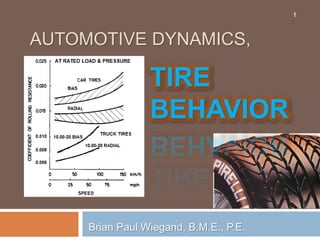
  • 1. AUTOMOTIVE DYNAMICS, Brian Paul Wiegand, B.M.E., P.E. 1 TIRE BEHAVIOR
  • 10. TIRE BEHAVIOR, TRACTION: MATERIAL 10 TIRE TRACTION: MATERIAL
  • 12. TIRE BEHAVIOR, TRACTION: MATERIAL 12 If the elongation under load, and the subsequent unloaded contraction, of a rubber sample were plotted on a scale more appropriate to the material’s unique behavior, then the result would be more like: This diagram reveals yet another curious aspect of the nature of rubber: high “hysteresis”. Most materials subjected to cyclical stress at sufficient levels will exhibit some conversion of mechanical energy to thermal energy, but rubber does so abundantly at relatively low stress levels; the area between the “loading” and the “unloading” curves represents the magnitude of this energy loss.
  • 13. TIRE BEHAVIOR, TRACTION: MATERIAL 13 Having noted how unusual rubber is in its elasticity, hysteresis, and other properties; we now have some clues as to the reasons for that unusual frictional behavior known as tire traction. At the small scale level of the contact area between tire and road the situation looks like (greatly enlarged):
  • 18. TIRE BEHAVIOR, TRACTION: STRUCTURE 18 TIRE TRACTION: STRUCTURE
  • 19. TIRE BEHAVIOR, TRACTION: STRUCTURE 19
  • 20. TIRE BEHAVIOR, TRACTION: STRUCTURE 20
  • 21. TIRE BEHAVIOR, TRACTION: STRUCTURE 21
  • 22. TIRE BEHAVIOR, TRACTION: STRUCTURE 22
  • 23. TIRE BEHAVIOR, TRACTION: STRUCTURE 23
  • 24. TIRE BEHAVIOR, TRACTION: STRUCTURE 24
  • 25. TIRE BEHAVIOR, TRACTION: STRUCTURE 25
  • 26. TIRE BEHAVIOR, TRACTION: STRUCTURE 26
  • 27. TIRE BEHAVIOR, TRACTION: STRUCTURE 27 …is the circle whose circumference is equal to the periphery of the tire cross- section as shown. Also shown in the figure are various other tire characteristics (dimensions): S = Circumference / π = Periphery / π
  • 28. TIRE BEHAVIOR, TRACTION: STRUCTURE 28
  • 29. TIRE BEHAVIOR, TRACTION: STRUCTURE 29
  • 30. = Tire section aspect ratio (dimensionless). SN = Tire nominal section width (mm). TIRE BEHAVIOR, TRACTION: STRUCTURE 30 The Rhynes Equation is very related to the Michelin Formula which is used to estimate the width of the tire tread “tw” (when lacking a measured value). The Michelin Formula is: Where: tw = Tire tread width, assumed constant with load (in). This equation was developed by a regression analysis of a large selection of common road tires (and therefore is not valid for uncommon size and type tires). Since the Rhynes Equation incorporates the Michelin Equation into its formulation it has the same limitation.
  • 31. TIRE BEHAVIOR, TRACTION: STRUCTURE 31
  • 32. TIRE BEHAVIOR, TRACTION: STRUCTURE 32
  • 33. TIRE BEHAVIOR, TRACTION: LATERAL 33 TIRE TRACTION: LATERAL μy = b – mN
  • 35. TIRE BEHAVIOR, TRACTION: LATERAL 35 Fy = (b-mN)N = bN – mN2
  • 38. TIRE BEHAVIOR, TRACTION: LATERAL 38 The presence of a lateral force on a tire not only causes a distortion of the tire carcass diminishing the tire/road area contact, but there are other effects as well. When a tire moving with velocity “Vo” encounters a side load there is a consequent sideways motion. The resultant new net motion “V” is the combination of the original motion “Vo” and the motion resulting from the side load. The angle “ψ” between this new direction “V” and the original direction “Vo” is called the “slip angle”. This term is a misnomer as it gives an erroneous impression; the tire is not necessarily slipping or sliding in the direction of the side load. What is actually happening is that there are a series of small lateral movements “dy” of the tire due to the cyclical distortion of portions the carcass as those portions come into contact with the road as the tire rolls forward. The combination of the original forward rolling velocity and all those infinitesimal “side steps” results in the new velocity direction “V”.
  • 43. TIRE BEHAVIOR, TRACTION: LATERAL 43 “…lateral…force may be thought of as the result of slip angle, or the slip angle as the result of lateral force…” (Milliken, William F., and Douglas L. Milliken; Race Car Vehicle Dynamics, Warrendale, PA; SAE R-146, 1995, pg. 19.)
  • 44. TIRE BEHAVIOR, TRACTION: LATERAL 44 Since the drift angle/lateral force relationship is dependent upon quite a few parameters (inflation pressure, normal load, etc.), it is common to look at functions which constitute only a partial differential of the total relationship (for which no one has yet established a complete definitive formulation based on physics*) in order to achieve a degree of understanding. If the tire drift- angle/lateral-force partial differential function is plotted the result looks like:
  • 46. TIRE BEHAVIOR, TRACTION: LATERAL 46 If matters were just as simple as the previous figure then understanding of tire behavior would be very easy. However, the potential or maximum lateral force that a tire can supply, and the drift angle associated with that force, is dependent on many parameters. The lateral force potential is primarily influenced by normal load, longitudinal load*, camber angle (which can change with roll), roll steer (which can be the result of normal load and camber change with roll, but toe in/out can also change with roll), tire type (size, carcass type and material, rubber type, tread design, aspect ratio), inflation pressure, wheel rim width, road material and surface (smooth, rough, dusty, etc.), weather (rain, snow, ice), temperature (road surface, ambient, and of the tire itself), and the speed of the vehicle (all basic tire coefficients of traction are somewhat speed dependent; the same lateral force will produce a smaller drift angle at high speed than at low speed**). While all these factors are significant, only tire type, normal load, long & lat force, inflation pressure, temperature, and speed are fundamental tire behavior and will be discussed herein; the rest has to do with tire/suspension interaction.
  • 47. TIRE BEHAVIOR, TRACTION: LATERAL 47 To illustrate the effect of normal load on lateral resistance and drift angle for a specific tire and inflation pressure a plot such as below may be used. Note that it is essentially like the previous figure except that there are now a large set of “Fy, ψ” functions which serve to represent an infinite variation; any change in normal load alters the “Fy, ψ” relation, but these five example curves may suffice as the intermediate possibilities can be approximated by interpolation:
  • 48. TIRE BEHAVIOR, TRACTION: LATERAL 48 Actually, the previous figure is a poor way to illustrate this behavior, which is better shown by the following actual data plot of lateral force vs. normal load for a 6.00x16 bias tire inflated to 28 psi (193 kPa):
  • 49. TIRE BEHAVIOR, TRACTION: LATERAL 49 Another way of looking at tire lateral traction force behavior is presented in this figure. This figure is somewhat like the previous, only now the lateral traction force “Fy” is normalized by “dividing out” the now constant normal load “N”, which of course results in the effective lateral traction coefficient “μy” (“μy = Fy/N”). This allows for the addition of a completely new type of extra information regarding the interaction of the lateral force with the longitudinal force which is indicated by the degree of “longitudinal slip” symbolized as “S” : Before this interaction can be explored in greater detail it is necessary to first consider the generation and behavior of the longitudinal traction force…
  • 50. TIRE BEHAVIOR, TRACTION: LONGITUDINAL 50 TIRE TRACTION: LONGITUDINAL The “traditional” tire lateral traction model accounts for change in normal load and change in contact area (“curl up”) effect on the lateral traction coefficient, but the “traditional” way of dealing with the longitudinal coefficient of traction has been simply to choose some seemingly appropriate constant value and make do with that. However, since the equation giving the traction coefficient variation with contact pressure is known, it would seem that the only info needed to relate the longitudinal coefficient of traction “μx” to normal load “N” is an equation relating the contact area to normal load. There is an equation in existence which does relate the contact area “Ac” to normal load, but it is relatively unknown. This equation was inspired by a concept presented by Prof. Dixon (Suspension Geometry and Computation, Chichester, UK; John Wiley & Sons Ltd, 2009, ISBN 978-0- 470-51021-6, pg. 85), then developed by Mr. J. Todd Wasson of Performance Simulations, and finally refined by this instructor.
  • 51. TIRE BEHAVIOR, TRACTION: LONGITUDINAL 51 That Dixon-Wasson-Wiegand tire-road gross contact area equation is: Where: Ac = Tire to ground plane gross contact area (in2) Lc = Tire to ground contact area length (in). tw = Tire tread width, assumed constant with load (in). Ri= Tire no-load inflated radius (in). d = Tire vertical deflection under load (in).
  • 52. TIRE BEHAVIOR, TRACTION: LONGITUDINAL 52 Of course, to calculate the area “Ac” requires the vertical tire deflection “d” under normal load “N” (“Nokian” Equation*)… Where: N = The normal load on the tire (lb). KZ = Tire vertical stiffness (lb/in). d0 = Tire deflection function “y-intercept” value (in). *Of course, this is known as the “Nokian” Equation to just a few Scandinavian researchers. To everyone else this is just the old tire vertical spring or linear deflection equation.
  • 53. TIRE BEHAVIOR, TRACTION: LONGITUDINAL 53 Which in turn requires knowledge of the tire vertical spring constant “Kz” (Rhynes Equation)… Where: KZ = Tire vertical stiffness (kg/mm). Pi = Tire inflation pressure (kPa). = Tire section aspect ratio (dimensionless). SN = Tire nominal section width (mm). DR = Wheel rim nominal diameter (mm). Note the “(-0.004 + 1.03) SN” term; this term when stand-alone is actually the next equation and is known as the Michelin Formula…
  • 54. Where: tw = Tire tread width, assumed constant with load (in). = Tire section aspect ratio (dimensionless). SN = Tire nominal section width (mm). This formula was developed by a regression analysis based on data from a large group of common passenger car tire sizes. Therefore this formula does not work very well for unusual size tires or tires that do not fit within the passenger car tire norm. Since the Rhynes Equation incorporates the Michelin Formula within its formulation then it also is subject to the same limitations. (The “0.03937” is a Metric to English units conversion factor.) TIRE BEHAVIOR, TRACTION: LONGITUDINAL 54 And knowledge of the tread width “tw” (Michelin Formula)…
  • 55. TIRE BEHAVIOR, TRACTION: LONGITUDINAL 55 All the parametric information necessary to plug into those four equations for determining a specific tire’s “contact area = f(normal load)” is contained in a tire’s “P-Metric” designation as inscribed on the sidewall. Determination of the contact area “Ac” under normal load “N” provides the contact pressure “Pc ” (= “N/Ac”) so that the peak longitudinal coefficient of traction can be obtained by the Koutný Formula: μx = a Pc n In order to generate a realistic variation with contact pressure the following exposition will utilize an example tire of designation “P152/92R16”, “a” will be set to “15.7369” (English psi units, for Metric kPa units use “58.2587”), and “n” will be set to “-0.67791” (a Koutný value, presumed typical): μx = 15.7369 (Pc)-0.67791
  • 56. TIRE BEHAVIOR, TRACTION: LONGITUDINAL 56 There are a number of “rules of thumb” that also attempt to define the relationship between the peak longitudinal coefficient of traction and the normal load; these may be useful for comparison with the equation. One of these “rules of thumb” is given by Prof. Gillespie: “…as load increases the peak and slide (traction) forces do not increase proportionately…in the vicinity of a tire’s rated load… (the traction) coefficients will decrease…0.01 for each 10% increase in load”. There is a similar “rule of thumb” attributed to Formula 1 competitors (source unknown) which may be paraphrased as: “…for every +5.82% increase in contact pressure there will be a -1.00% decrease in the traction coefficient…”. The variation of the peak longitudinal coefficient of traction with normal contact pressure as per the Koutný model and the “rules of thumb” may be graphically presented as
  • 57. TIRE BEHAVIOR, TRACTION: LONGITUDINAL 57 Fx = (a Pc n)N
  • 58. TIRE BEHAVIOR, TRACTION: LONGITUDINAL 58 As was the case with the lateral traction force potential, the longitudinal traction force potential also varies with inflation pressure, and will form a family of curves for a particular tire:
  • 59. TIRE BEHAVIOR, TRACTION: LONGITUDINAL 59 Also as was the case for lateral traction, there is a tire deformation that accompanies longitudinal traction loadings, which may be illustrated as per the figure: In the figure, for the conditions of acceleration and braking, the vertical force “Fz” (the resultant of the contact area vertical pressure distribution and equal to “N”) times the offset arm “d” constitutes the rolling resistance. The presence of longitudinal traction forces for acceleration (“Fx”) and braking (“-Fx”) both increase rolling resistance, but not to the exact same extent. Acceleration and braking generate different longitudinal shear stress distributions (compression vs. tension), which interact with the vertical contact stress distribution, which affects the rolling resistance
  • 60. TIRE BEHAVIOR, TRACTION: LONGITUDINAL 60 As illustrated, as each tire tread segment rolls into contact with the ground, there is a longitudinal stretching or compression of that segment, followed by a contraction or expansion as the segment rolls up out of contact. It is this cyclical distortion of the tread that gives the appearance of “slip”, which is to say the speed of rotation of the tire “ω” seems out of synch with the velocity “V”. “Slip” may be represented as “%S”, or just “S”. The tire segment in contact with the road and under traction stress is generally not in motion with respect to the road (although some portions of the contact area may be); on the whole the tire contact area may be regarded as actually being “static” with respect to the road.
  • 61. TIRE BEHAVIOR, TRACTION: LONGITUDINAL 61 Just as the drift angle “ψ” was proportional to the lateral force “Fy”, the apparent slip “%S” is proportional to the longitudinal force “Fx”, the potential for which depends on the normal load “N”. The following figure shows the relationship between the longitudinal traction force “Fx” and slip “%S” for some constant normal load “N” (note the similarity to the previous lateral traction force “Fy” vs. drift angle “ψ” figure):
  • 62. TIRE BEHAVIOR, TRACTION: LONGITUDINAL 62 This next figure shows how this relationship can vary for different normal loads; it is based on a plot made by use of the BNP (Bakker-Nyborg- Pajecka) tire model using parameters empirically obtained for a particular truck tire and inflation pressure; some model results are over-plotted with their empirical counterparts to indicate the degree of model veracity. Note that the proportional limit is indicated at around 10% slip (normal road driving slip is generally under 3%).
  • 63. TIRE BEHAVIOR, TRACTION: LONGITUDINAL 63 In a way analogous to the lateral case of the lateral traction force “Fy” variation with normal load “N” per drift angle “ψ” family of curves, it should be possible to plot longitudinal traction force “Fx” variation with normal load “N” per percent slip “%S” to produce a similar family of curves. However, no such plot could be readily found in the literature. Therefore, the data inherent in the previous figure was replotted in an attempt to construct such a figure
  • 64. TIRE BEHAVIOR, TRACTION: LONGITUDINAL 64 Just as was done earlier for the lateral traction force vs. drift angle functions at various normal loads, the longitudinal counterpart can also be normalized and extended over four quadrants. Again there is indication of an interaction between the long and the lat forces, only now it is the lateral force effect that is recognized through its drift angle “ψ” This interaction of the long and the lat will now be explored more thoroughly…
  • 65. TIRE BEHAVIOR, TRACTION: LAT + LONG 65 TIRE TRACTION: LONGITUDINAL & LATERAL TOGETHER The question now presents itself: how do we “synchronize” the longitudinal and lateral traction functions so that they coherently represent the same tire? This is not, or should not, be a problem if all the necessary tire coefficients are properly determined by empirical means for use in a unified tire model like the “Magic” or “LuGre” models, but it does become a question if the attempt is made to construct a model for a theoretical tire using just the simple relationships expounded on herein. Of course, the establishment of the maximum longitudinal/lateral traction forces that a tire could generate for a particular inflation pressure, normal load, etc., would go a long way toward that construction, but the result can only be used for exposition and conceptual thinking. For realistic engineering determinations of what performance levels a detailed design could achieve on a specific road course, only a model such as the “Magic”, or perhaps the “LuGre”, can truly suffice.
  • 66. TIRE BEHAVIOR, TRACTION: LAT + LONG 66 A tire may experience an essentially purely longitudinal or a purely lateral traction loading under certain limited circumstances, such as a drag racing or skid pad simulation; but generally a tire undergoes a simultaneous combination of lateral and longitudinal loading. If the maximum loading a tire could undergo were equal in either direction, then the maximum resultant combination of longitudinal and lateral traction forces that a tire could generate would be obliged to fall within a “traction circle”, or at least for simplicity’s sake the situation is often portrayed that way. Actually, because tire traction behavior is anisotropic, the situation is much more accurately modeled as a “traction ellipse”, although even that is not perfect.
  • 67. TIRE BEHAVIOR, TRACTION: LAT + LONG 67 When the lateral/longitudinal traction relationship is portrayed as a circle it allows for some very simple determinations. For instance, note that the two orthogonal traction forces “Fx” and “Fy” must always combine to form the resultant force “Fr” as per: When utilizing the circle model, this resultant force “Fr” can’t exceed the circle radius or maximum traction force “R”, if a skid is not to set in. So, using this simple relation, if “R” is 560 lb (254.0 kg), and “Fy” is 300 lb (136.1 kg), then in order for the particular tire considered to not go into a skid “Fx” can only go up to: = So simple, but so far from realistic…
  • 68. TIRE BEHAVIOR, TRACTION: LAT + LONG 68 In the quest to keep things as simple as possible, but with a closer correspondence to reality, the ellipse model was developed. An over-plot comparison of the circle and ellipse models for the same tire would look as follows:
  • 69. TIRE BEHAVIOR, TRACTION: LAT + LONG 69 The major axis of the ellipse is “2a” in length, while the minor axis is “2b”. In this tire traction model the “a” corresponds to the maximum longitudinal traction available, and the “b” corresponds to the maximum lateral traction available. Note that the ellipse properly represents the passenger car tire relation between maximum longitudinal and lateral traction forces in that “a > b” (*see refs): a = Fx max b = Fy max So, with “a” and “b” quantified, a property called the “eccentricity” of the ellipse can be calculated: The eccentricity “e” represents the ratio of the “c” dimension, which is the distance of the “foci” from the center (origin) divided by the “a” dimension (one half the major axis):
  • 70. TIRE BEHAVIOR, TRACTION: LAT + LONG 70 The significance of the tire traction ellipse lies in the fact that no combination of longitudinal and lateral tire traction forces, i.e. no resultant traction force, can be so great that if plotted to scale it would project beyond the ellipse periphery. The need for any traction force so great that it would fall on the ellipse periphery is indicative of impending skid. Any point on the periphery of an ellipse must conform to the ellipse equation: So, if “Fx max” (“a”) = 629.4 lb (285.5 kg) and “Fy max” (“b”) = 498.5 lb (226.1 kg), then when “Fy” = 300.0 lb (136.1 kg) the maximum amount of “Fx” tolerated before a skid would ensue is:
  • 71. TIRE BEHAVIOR, TRACTION: LAT + LONG 71 A traction ellipse such as shown so far holds only for a particular tire on a particular surface at specific normal load, inflation pressure, velocity, and temperature. These limitations can be countered some- what by normalizing the longitudinal & lateral forces, by assuming a constant inflation pressure & temperature (due to the attainment of thermal equilibrium), and by placing the “secondary” matter of velocity effect aside for the moment. This gives us the slightly more useful traction ellipse
  • 72. TIRE BEHAVIOR, TRACTION: LAT + LONG 72 A 3D plot of a specific tire’s traction potential from “N = 0” to its absolute maximum load capacity “N = Lcap” at its absolute maximum inflation pressure “Pcap” could be constructed. If so, the result would look something like a hemispheroid (or a grapefruit serving) as shown:
  • 73. TIRE BEHAVIOR, TRACTION: LAT + LONG 73 If enough data were available for a specific tire to construct a volume as shown for “N = 0” to “N = Lcap” for each “Pi” increment of, say, 5 psi throughout the working pressure range, then this perhaps would constitute enough data for utilization in a full quantitative automotive performance simulation. Such a simulation would have to contain interpolation routines for the determination of appropriate data values that lie between the known “N” data levels, and further routines to modify that interpolated data to account for the effects of temperature, velocity, and camber. All things considered, that might be enough to make utilization of the “Magic” or other such complex formulations unnecessary*. Moreover, if one’s concern is on a less sophisticated level, i.e. - “is there enough traction to complete a particular maneuver?”, then reference to even an appropriate tire traction ellipse may not be necessary; if the resultant of the “Fx” and “Fy” forces (“[Fx 2 + Fy 2]0.5”) is less than “0.3 N” in value then the answer is “yes”. It’s only when a vehicle is being driven hard, certainly at the point of loss of control (skid), that tire traction ellipse use becomes necessary.
  • 74. TIRE BEHAVIOR 74 Up to this point only the well established basics of tire behavior have been discussed. However, now the discussion will involve some aspects of tire behavior that are less well established, including some points that are totally speculative. Perhaps some day one of the students in today’s class will be instrumental in exploring and clarifying some of these speculative areas, advancing the state of the art…but probably not…
  • 75. TIRE BEHAVIOR: TEMPERATURE 75 TEMPERATURE EFFECTS The effect of temperature is often ignored; either it is considered inconsequential or a benign condition of thermal equilibrium is assumed. However, there are cases when the blind discounting of temperature can be disastrous. The variation with temperature of material properties, mostly the properties of rubber, causes significant variation in tire behavior. Traction, rolling resistance, and inflation pressure are all affected, which in turn causes other effects (%slip, slip angle, cornering stiffness, fuel economy, wear, vertical spring constant, etc.) Temperature and inflation pressure are very closely interrelated as per the Ideal Gas Law: PV = n R T
  • 76. TIRE BEHAVIOR: TEMPERATURE 76 In that equation the gas pressure “P” (in “atmospheres”) and volume “V’ (in liters) are related to the gas temperature “T” by the factors “n” (the amount of gas in “moles”) and “R” (the Universal Gas Constant: 0.08207 liter-atm/mole-oK). Ignoring the small changes in tire volume “V” with inflation pressure “P” (“V” is constant) means that “P = (nR/V) T” where “nR/V” is a constant; tire pressure varies in a direct linear relation with tire temperature:
  • 77. TIRE BEHAVIOR: TEMPERATURE 77 Since the tire vertical spring constant “Kv” varies with pressure in accord with the Rhynes Equation, then the deflection under load will vary, which in turn affects the tire-road contact area. Therefore, increased “T” means increased “Pi” and “Kv”, which in turn leads to decreased “d” and “Ac”. And that ultimately means decreased rolling resistance, which means improved fuel economy, but also less traction…However, all of that has been covered by the basic tire equations already discussed, but the tire mechanical effects caused by temperature variation aren’t the whole story; there are material effects as well. Rubber energy dissipation (hysteresis) and traction coefficient varies directly with temperature in a very non-linear fashion
  • 78. TIRE BEHAVIOR: TEMPERATURE 78 The total effect of the combination of the mechanical and the material aspects leads to somewhat puzzling statements such as*: “…increase in energy dissipation that accompanies an increased load causes the temperature of the tire to rise…results in lower hysteretic loss coefficient…as a result the coefficient of rolling resistance often decreases somewhat with increasing load…” There are forms of automotive endeavor in which temperature levels play a significant, and complicated, role. For instance, Formula 1 and Indy car tires require operation within a narrow temperature band for optimum performance; per an authoritative source**: “Modern race tire compounds have an optimum temperature for maximum grip. If too cold, the tires are very slippery; if too hot the tread rubber will ‘melt’; in between is the correct temperature for operation.”
  • 79. TIRE BEHAVIOR: TEMPERATURE 79 For racing tires the increase in temperature with velocity and hard use is planned for, and if laps have to be run at reduced speed under a safety flag, or during a rolling start, then it is not unusual to see the cars alternately darting hard right and left as the drivers try to keep their tires at optimum temperature as they wait for all out racing to recommence. Possibly one of the worst scenarios that can occur in racing is to be caught with rain tires installed as the track starts to dry out and there is no chance of a pit stop for tire replacement; the “softer” compound rain tires are certain to overheat unless the driver commences driving far less aggressively, which is a tactic not likely to place him on the podium.
  • 80. TIRE BEHAVIOR: INFLATION PRESSURE 80 It has already been discussed how tire inflation pressure will affect the vertical stiffness, and other measures of tire stiffness as well, such as the “Cornering Stiffness”* or the lateral traction coefficient “m” (which is an inverse measure of stiffness). As noted, such changes cause a cascade of other changes; a change in vertical stiffness will affect the vertical deflection under load (and therefore the rolling radius**), which in turn will affect tire-ground contact area (and therefore traction), and that leads to changes in rolling resistance (and therefore fuel economy), heat generation, and temperature. And, of course, this tends to run in a full cycle, as temperature will, in turn, affect the inflation pressure. Here we are going to discuss some of these consequences of inflation pressure that have not been adequately dwelt on before, like rolling resistance…
  • 81. TIRE BEHAVIOR: INFLATION PRESSURE 81 The effect of inflation pressure variation on rolling resistance as reflected in the Stuttgart Rolling Resistance Formula Coefficients, “Static” (Cs) and “Dynamic” (CD)…
  • 82. TIRE BEHAVIOR: INFLATION PRESSURE 82 The variation in tire-road contact area versus inflation pressure (note that without temperature or normal load change the longitudinal tire traction may be considered as varying in exact proportion to the change in area) may be illustrated as:
  • 83. TIRE BEHAVIOR: INFLATION PRESSURE 83 Increasing inflation pressure will also cause some expansion of the tire circumference, although such expansion usually is very small*. The situation is depicted As the inflation pressure “P” increases the force “F” pushing the tire semi-sections apart; the force is equal to the pressure times the horizontal plane area: “F = P A”. Expressed in differential form this relation may be expressed as: This causes corresponding stress “dS” and strain “dε” differentials in the tire periphery (tread): By definition “dL/L” is substituted for “dε”, and the expression rearranged: The stress “dS” is equal to “2 dF/2” (“dF”) over the tire tread cross-sectional areas “2 tt tw”, or “dS = dF/2 tt tw”, which allows for the following substitution and simplification…
  • 84. TIRE BEHAVIOR: INFLATION PRESSURE 84 Remember that “dF = dP A”, and note that “A = 2 R tw”; this allows for the following substitution and simplification: Since the tire circumference “C” (“2 π R”) is equal to “2 L”, the relation of the tire radius “R” to “L” is “2 π R = 2 L” or “π R = L”. Therefore “L = π R” and “dL = π dR”; substitute for “L” and “dL”: Remember that this is only for rough estimation as this simplified relationship was made by ignoring the stiffness contribution of the sidewalls, etc. However, the final relation for determining the difference in an inflated no-load tire radius due to an inflation pressure change is:
  • 85. TIRE BEHAVIOR: INFLATION PRESSURE 85 The use of this equation produces an inflated no-load tire radius (upper plot line) versus inflation pressure plot as per:
  • 86. TIRE BEHAVIOR: VELOCITY 86 An authoritative source states “In preliminary performance calculations the effect of speed may be ignored (with respect to rolling resistance)”*. However, the rolling resistance variation with speed (velocity) is explicitly known via the Institute of Technology in Stuttgart formula of circa 1938: VELOCITY EFFECTS CR = CS + 3.24 CD (V/100)2.5 Given coefficient values such as those of previous figures, but appropriate for the specific tires concerned, a vehicle’s rolling resistance can be reasonably determined for a wide range of velocity variation, so no ignoring of the velocity effect on rolling resistance is necessary. However, there are other sources which state “Velocity does not significantly affect cornering stiffness of tires in the normal range of highway speeds”**, and “To a first order, tire forces and moments are independent of speed”***.
  • 87. TIRE BEHAVIOR: VELOCITY 87 However, there are definite decreases in longitudinal traction coefficients with velocity which may not be well defined, but for which there is considerable empirical data, such as that contained in the following table for longitudinal traction*:
  • 88. TIRE BEHAVIOR: VELOCITY 88 Both the static and dynamic coefficients of traction are functions of velocity, which is contrary to the Coulomb friction model. A plot of the static (rolling) and dynamic (skid) coefficients as a direct function of velocity is as follows*:
  • 89. TIRE BEHAVIOR: VELOCITY 89 How the variation in traction with velocity affects the longitudinal traction/longitudinal “slip” relationship may be depicted in a general way as follows: [This figure is just a “cartoon” , an ad hoc adaptation of an illustration found in Harned, Johnston, and Scharpf; “Measurement of Tire Brake Force Characteristics as Related to Wheel Slip (Antilock) Control System Design”, SAE Paper 690214, 1969, so no one should attempt to use it for anything quantitative.]
  • 90. TIRE BEHAVIOR: VELOCITY 90 In acceleration and deceleration the variation in both the normal load and velocity affect the maximum longitudinal traction available. However, it is more important to account for the effect of both “N” and “V” on “μx” in a braking simulation such as “MAXDLONG.BAS” than it is in an acceleration simulation such as “MAXGLONG.BAS”. A braking simulation commences at a high “V”, and the determination of the maximum traction available for deceleration is very much dependent on that “V”. An acceleration simulation commences at zero “V”, and as the velocity increases the need for determination of the maximum traction available decreases because the propulsion force available for acceleration is also decreasing; this is contrary to the braking situation wherein the brake force available for deceleration may actually increase with time. Therefore this instructor chose to develop an expression for the variation of “μx” (a.k.a. “μpeak”, maximum longitudinal traction coefficient) with regard to both “N” (“Pc”) and “V”: “μx = f(N, Pc)”. A number of reference documents were utilized to develop a suitable expression for “μx = f(V)”, then combined with the known “μx = f(Pc)”…
  • 91. TIRE BEHAVIOR: VELOCITY 91 …resulted in: The form of this equation may be generally applicable, but it just represents the specific tire (152/92R16 @ 45 psi) for which it was developed; a different version of this equation must be developed to represent any other tire/inflation pressure. This equation for determination of “μx” was incorporated in the traction subroutine of the “MAXDLONG.BAS” program. An indication of the validity of this equation may be gleaned by consideration of how the equation performs as the variables “N” and “V” are varied independently:
  • 92. TIRE BEHAVIOR: VELOCITY 92 Increased velocity also means increased flexing of the tire tread per unit time, thereby generating more heat flow and raising the tire temperature, as indicated per the following table*: VELOCITY and TIRE TEMPERATURE * Woodrooffe, and Burns; “Effects of Tire Inflation Pressure and CTI on Road Life and Vehicle Stability”, Proceedings of the International Forum for Road Transport Technology, pp. 203-221, pg. 205.
  • 93. TIRE BEHAVIOR: VELOCITY 93 The increased temperature through the material properties of rubber has its own effect on traction, but complicating matters is the subsequent daisy chain of structural consequences: higher inflation pressure, increased vertical stiffness, decreased deflection under load, decreased tire-road contact area, leading to a further decrease in traction. Given all this action and reaction it is understandable that tire researchers have historically had difficulty in trying to separate such things as velocity effects from pressure effects; on the tire testing machine the two effects go hand-in-hand; such hard to separate parameter interactions have been the main reason for the slow progress in the understanding of tire behavior. Since an increase in tire temperature results from increased tread flexure, velocity is not the only driving parameter behind that effect. Varying longitudinal/lateral accelerations will also cause tread flexure resulting in temperature increase; generally, the harder a vehicle is driven the higher tire temperatures will raise. It also follows that the more underinflated a tire is, the higher its temperature will climb; for optimum tire life it is wise to maintain tire inflation pressures in accord with manufacturer’s specifications.
  • 94. TIRE BEHAVIOR: VELOCITY 94 Velocity also directly affects the vertical spring constant of the tires, and seemingly in a manner that leads to all sorts of confusion. Taylor, Bashford, and Schrock have demonstrated that the measured value of a tire vertical spring constant “Kv” can vary considerably depending upon the method used to do the measuring. The most common test method, which accounts for the vast majority of measured vertical spring constant data, is the “Load-Deflection” (LD) method. This method, along with four other methods, was evaluated by these researchers regarding the “Kv” of a 260/80R20 agricultural (!) tire: VELOCITY and TIRE VERTICAL SPRING CONSTANT •Load-Deflection (LD). •Non-Rolling Vertical Free Vibration (NR-FV). •Non-Rolling Equilibrium Load Deflection (NR-LD). •Rolling Vertical Free Vibration (R-FV). •Rolling Equilibrium Load-Deflection (R-LD).
  • 95. TIRE BEHAVIOR: VELOCITY 95 It seems that the major distinctions between the methods involve whether the test is static/quasi-static (response to load) or dynamic (response to impact/vibration). This instructor believes this distinction is the key to understanding what seems to be a lot of confusing and conflicting test results, beginning with the Taylor, Bashford, and Schrock paper and many of their cited references, and ending with a later paper by Kasprzak and Gentz whose main result is in seeming direct contradiction to Taylor, Bashford, and Schrock*. This instructor’s personal resolution of the matter, based mainly on intuition unsupported by any solid substantiation, is that there may be two types of vertical spring rate involved. One type of stiffness may be that measured by static/quasi-static load response methods (LD); the other type of stiffness may be that measured by dynamic impact/vibration response methods (FV**). The static/quasi-static stiffness decreases with increasing velocity asymptotically up to a certain speed dependent on the particular tire/inflation pressure concerned. The impact/vibration stiffness increases with increasing velocity (due to inertial effects). To say more than that would require further study, but it would seem that the static/quasi-static vertical stiffness would be suitable for use in determining the tire rolling radius variation due to “weight transfer” as used in acceleration/braking simulations, while the impact/vibration stiffness would be suitable for use in suspension shock/vibration studies.
  • 96. TIRE BEHAVIOR: VELOCITY 96 VELOCITY, CENTRIFUGAL FORCE, & TIRE ROLLING RADIUS The rolling radius variation with velocity due to centrifugal force is determinate, unlike some matters just dealt with. A tire under load tends to “expand” back to its full no-load inflated radius dimension (“Ri” or “Di / 2”) due to centrifugal force as the velocity increases; accompanying this is a true expansion (stretching of the carcass) also due to centrifugal effect, but such stretching tends to be relatively small in most cases and has already been dealt with. An extreme example of tire rolling radius “expansion” would involve the huge racing slicks (usually bias, a.k.a. cross-ply, without “belts”) that some “dragster” types use. As an “AA” fuel dragster accelerates off the line the huge rear slicks, usually Hoosier brand, expand until the rear of the dragster appears to be “standing on tip toes”. This “standing on tip-toes” behavior has been witnessed and photographically documented innumerable times. This tire behavior is by design; the enlarged rolling radius at high speed is intended to change the overall drive ratio of the vehicle, compensating for the fact that such dragsters tend to be direct drive or only two-speed.
  • 97. TIRE BEHAVIOR: VELOCITY 97 Such tire “expansion” is less extreme and considerably less noticeable for passenger cars. The following figure shows a measured increase in rolling radius with speed (to about 150 kph, or 93.2 mph) for a 5.60×5 cross-ply (0-0.43 in) and a 155SR15 radial (0-0.15 in); both tires are at 22 psi (152 kPa) pressure and under 661 lb (299.8 kg) normal load:
  • 98. TIRE BEHAVIOR: VELOCITY 98 The previous figure was utilized as the inspiration for the development of a “tire rolling radius” subroutine for use in the “MAXGLONG.BAS” automotive acceleration program. A 1984 parameter dump during successive runs of that program revealed the following with regard to this tire expansion subroutine function:
  • 99. TIRE BEHAVIOR: VELOCITY 99 The present methodology for the static deflection recovery is derived as follows… The mass of the deflected portion of the tire periphery “m1-3” is pushed back against the normal force reaction “N” by the centrifugal acceleration “V2/R” giving rise to the radius recovery increment “dRrecovery”: Using weight as a measure of mass requires the substitution: The weight “W1-3” is equal to the volume “tt tw Lc” times the density “δ”, where “Lc” is equal to “1.24 Ri Cos-1((Ri-d)/Ri)”; making the substitution:
  • 100. TIRE BEHAVIOR: VELOCITY 100 Substitute “386.088 in/sec2” for “g”, add “mph to in/sec” conversion constant “17.6”, and rearrange slightly: Although the effect is usually minor, there is a real expansion (strain) of the tire periphery that causes a further increase in the effective tire radius with increasing velocity. This tire expansion radius increment “dRexpand” runs concurrent with the recovery increment, at least until the static deflection is fully counteracted which is when “dRrecovery” ceases. The expansion model is as per the next figure, which is a free body diagram of a half periphery of the tire: The periphery stress resulting from the centrifugal force “F” can be determined by a study of this free body diagram.
  • 101. TIRE BEHAVIOR: VELOCITY 101 This study begins with: The ½ periphery length “L” is equal to half of “2 R π”, so: Therefore “R” can be expressed as: And the radius expansion increment as: Since the strain “ε” is equal to “dL / L” by definition the substitution for “dL” may be made: Make use of the stress-strain relation “S = E ε” to substitute “S/E” for “ε”:
  • 102. TIRE BEHAVIOR: VELOCITY 102 Substitute “(F/2)/A” for “S”: Substitute “WL ω2 / g” for “F”: The weight “WL” of the tire tread sector “L” is equal to “L tw tt δ”, the CG coordinate “ ” of that sector is equal to “2 R / π”*, the angular velocity “ω” is equal to “V/Rr”, and the transverse tread area of the tire cords is estimated as “tw tt f”**; making the corresponding substitutions and simplifying results in: From earlier simple circular relations the length “L” is known to be equal to “R π”, which is now substituted for “L”: Simplify:
  • 103. TIRE BEHAVIOR: VELOCITY 103 Now some unit conversion factor (mph × 17.6 = in/sec) and constant value (g = 386.088 in/sec2) adjustments are required, and “R” becomes “Ri” as that radius better represents the general condition along the periphery “C” than “Rr”: As the velocity “V” increases the deflection recovery equation and the centrifugal expansion of the tread equation work together (are additive) in increasing the rolling radius “Rr” until the point is reached when “Rr = Ri” which signifies (approximately) total recovery of the initial static deflection. Beyond that point the centrifugal expansion carries on alone until the tire self-destructs. Of course, that seldom happens as velocities high enough to cause tire destruction by centrifugal stresses are reached only by vehicles such as LSRs.
  • 104. TIRE BEHAVIOR: VELOCITY 104 For passenger car tires true centrifugal expansion is very minor, especially if the tires in question have steel (“E ~ 29,000,000 psi”) or other high Modulus of Elasticity material belts. Most modern passenger car tires are radials and belted, but a bias tire dating from the 1945-1967 period might rely on only nylon and/or rayon cords for constraint (“E ~ 410000 psi or less”). It should perhaps be noted at this point that the exact value of the Modulus of Elasticity to be used for a calculation or simulation is not necessarily a “cut and dried” matter. Even for the same tire, the modulus value will vary depending on the use to which that value is to be put. For example, the Krylov and Gilbert equation for determining the critical velocity for “standing wave” formation was derived using a model of a longitudinal tire tread segment as a beam supported on springs. Even though a modern (c. 2003) passenger car tire (exact type unspecified) parametric value set served as input for their example calculation, the modulus value was only 171,304 psi (“3·107 N/m2”)*!
  • 105. TIRE BEHAVIOR: VELOCITY 105 This is a far cry from the modulus value for steel (29,000,000 psi), or any other conceivable tread belt material, but that is because the belts reside near the neutral axis of the beam model, and thus have no role in this particular calculation. The modulus value that Krylov and Gilbert used was some combination of the carcass cord and tread materials (Ref.: Enylon ~ 410,000 psi, Erubber ~ 500 psi)*, as was suitable for their purpose. If the calculation had instead been one of tire peripheral expansion in response to centrifugal force, then the modulus used would have been much higher, probably very close to the Modulus of Elasticity of the belt material**.
  • 106. TIRE BEHAVIOR: VELOCITY 106 Consider the result of a practical application of the recovery equations and the expansion equation as presented herein. The tire is the 1958 Dunlop RS4 6.00×16 bias tire (with inner tube) at 45 psi (310 kPa) under a 1238 lb (561.5 kg) normal load, resulting in a 0.84 in (21.3 mm) static deflection. The tire is presumed to be unbelted, and largely of nylon cord/rubber construction; the Modulus of Elasticity is taken as 450,000 psi (3·109 N/m2). An iterative spreadsheet calculation of the subject equation results looked as follows when plotted:
  • 107. TIRE BEHAVIOR: VELOCITY 107 The symbolism for the tire expansion due to inflation pressure through the expansion due to velocity equations is as follows: d = Tire vertical deflection under a normal load (in). δ = Tire tread cords/belts/rubber composite density (lb/in3) E = Tire tread Modulus of Elasticity (lb/in2). f = Tire tread cross-sectional area adjustment factor (dimensionless). Kv = Tire vertical spring rate (lb/in). P1 = Tire initial inflation pressure (lb/in2). P2 = Tire new inflation pressure (lb/in2). Ri = Tire inflated no-load radius (in). Rr = Tire rolling radius (in). tt = Tire tread thickness (in). tw = Tire tread width (in). V = Vehicle velocity (mph).